Math. Model. Nat. Phenom. Vol. , No. , 2012
3D data denoising using combined sparse dictionaries G. Easleya , D. Labateb1 and P. Negib a
b
System Planning Corporation, Arlington, VA 22201, USA Department of Mathematics, University of Houston, Houston, Texas 77204, USA
Abstract. Directional multiscale representations such as shearlets and curvelets have gained increasing recognition in recent years as superior methods for the sparse representation of data. Thanks to their ability to sparsely encode images and other multidimensional data, transformdomain denoising algorithms based on these representations are among the best performing methods currently available. As already observed in the literature, the performance of many sparsitybased data processing methods can be further improved by using appropriate combinations of dictionaries. In this paper, we consider the problem of 3D data denoising and introduce a denoising algorithm which uses combined sparse dictionaries. Our numerical demonstrations show that the realization of the algorithm which combines 3D shearlets and local Fourier bases provides highly competitive results as compared to other 3D sparsity-based denosing algorithms based on both single and combined dictionaries. Key words: Curvelets, denoising, nonlinear approximations, pursuit algorithms, shearlets, sparse approximations, wavelets. AMS subject classification: 42C15, 42C40
1. Introduction The notion of sparse representations has been one of the most pervasive and seminal concepts in the applied harmonic analysis and signal processing literature during the last decade. Intuitively, a representation is sparse if it allows one to efficiently approximate functions in a certain class using only a “small” number of terms when functions are expanded with respect to the representation. Sparsity can be exploited very effectively in denoising applications. In fact, constructing sparse 1
Corresponding author. E-mail:
[email protected]
1
G. Easley, D. Labate and P. Negi
3D data denoising using combined sparse dictionaries
representations for functions in a certain class entails the ability to efficiently capture their fundamental structures, hence enabling to extract the features of interest and remove the unwanted components. A transform-domain denoising algorithm exploits the concept of sparsity through the assumption that the true data are well approximated by a linear combination of few basis elements with respect to an appropriate representation. Hence, by preserving the few large-magnitude representation coefficients and discarding the rest, the true signal can be effectively estimated. This concept was formalized through the celebrated shrinkage algorithms originally introduced by Donoho and Johnstone [7, 10, 11, 12], which have been spectacularly successful in the signal and image processing community during the past 15 years. To illustrate this denoising strategy in the classical setting of additive white Gaussian noise, let us suppose that we want to recover f ∈ L2 (Rd ) from the noisy observations y = f + n,
(1.1)
where n is zero-mean white Gaussian noise with variance σ 2 . If the function f to be recovered is known to be sparse under an appropriate dictionary, say, orthogonal wavelets, then the classical shrinkage algorithm offers a simple yet very effective approach. This consists in: (i) applying the transform analysis operator, denoted by W, to the noisy data, (ii) applying a thresholding operator T and, finally, (iii) applying the inverse transform operator to obtain an estimator f˜ of f . That is, f˜ = W −1 T W f.
(1.2)
The performance of this estimation is closely related to the sparsity of the representation system. In fact, suppose that W is unitary and T is the soft thresholding operator, defined by Tτ (α) = sign(α)(|α| − τ )+ , where τ is a fixed parameter. In this case, Donoho and Johnstone [10] have shown that, if the m-term approximation error decays as ∥f − fm ∥2L2 ≤ C m−k ,
as m → ∞,
where fm is the m-term approximation of f , then there is a constant C ′ > 0 so that ) ( 2k 2 ˜ E ∥f − f ∥L2 ≤ C ′ σ k+1 , as σ → 0, where E is the expectation and σ is the standard deviation of the noise. For example, curvelets and shearlets are optimally efficient for representing smooth images with edges, so that curvelet-based and shearlet-based shrinkage algorithms are extremely effective for this type of data. However, data found in applications are usually complex and there is no single representation system that can optimally approximate all the features of interest. While curvelets and shearlets are very efficient for representing data with distributed singularities such as edges, Fourier bases are better at dealing with oscillatory features, usually described as texture. Therefore, it seems reasonable to consider combined representations made up of many different types of waveforms, each type having its own area of specialization. The idea of coding images as a multi-layered representation of a piecewise smooth layer and a texture layer is rather old [22, 28], but only more recently the concept of combined representations has been considered within the setting of sparse 2
G. Easley, D. Labate and P. Negi
3D data denoising using combined sparse dictionaries
data decompositions. In particular, one emerging approach is based on the concept morphological diversity (see discussion in [32, 34]), which assumes that data can be modeled as a sum: x=
K ∑
xk ,
k=1
where each morphological components xk of the data is sparse with respect to a given dictionary Φk . In addition, the various dictionaries satisfy a form of incoherence, that is, each components xk of the data is sparse with respect to a dictionary Φk , but not with respect to the other dictionaries Φℓ , for ℓ ̸= k. In this paper, we have focussed on 3D data denoising, which is an area of increasing interest for video restoration and preprocessing of biological data. For this task, some of the most competitive algorithms currently available are transform-domain algorithms which rely on the sparsity of advanced directional multiscale systems such as curvelets, shearlets and surfacelets [25, 30, 35]. As suggested above and as indicated by several recent results in the literature, the performance of many sparsity-based algorithm can be further improved by considering dictionaries which are obtained as appropriate combinations of several representations, each one specialized in different features of the data to be analyzed (e.g., textures and piecewise smooth regions). Following the general philosophy of morphological diversity, we have assumed that typical 3D data of interest (e.g. videos of natural scenery, biological data) are well represented through combined dictionaries based on wavelets, curvelets, shearlets and Fourier bases. Using this approach we have derived highly performing denoising algorithms which were validated through extensive numerical experiments. As a benchmark, our results were compared against standard and state-of-the-art denoising algorithms based on both single and combined dictionaries, showing that, in particular, the realization of our algorithm which combines 3D shearlets and local Fourier bases provides the best performance in terms of noise removal. The paper is organized as follows. In Section 2. we will briefly survey the theory of sparse representations and recall the construction of 3D shearlets, which are especially efficient for the representation of piecewise smooth functions of three variables. In Section 3. we present an algorithm for 3D data denoising which uses an appropriate combination of sparse representations. Finally, in Section 4. we present several numerical demonstrations of our denoising algorithm, and compare it against other standard and state-of-the-art denoising algorithms.
2. Sparse multidimensional representations Sparsity and sparse representations are leading concepts not only in the current signal and image processing literature, but also in a variety of areas such as inverse problems, numerical analysis and data mining. We will not attempt to comprehensively review this topic and its applications, but will only focus on the aspects which are most closely related to the problem of data denoising. We start with some basic definitions.
3
G. Easley, D. Labate and P. Negi
3D data denoising using combined sparse dictionaries
2.1. Sparse representations: beyond wavelets 2 d Let B = {bi : i ∈ I} be an orthonormal basis or even a Parseval frame ∑ for a subset U of L (R ), and, for f ∈ U , let us consider its expansion in B, that is, f = i∈I αi (f ) bi . The system B is said to provide a sparse representation of U if the sorted magnitudes of the expansion coefficients |α(f )||(i)| have rapid decay according to the power law
|α(f )||(N )| ≤ C ∥f ∥L2 N −s ,
as N → ∞,
where C > 0 is a constant independent of f . This implies that, letting fN be the approximation of f obtained by using the N largest coefficients of the expansion of f in B, the nonlinear approximation error, defined by ∥f − fN ∥2L2 , decays as ∥f − fN ∥2L2 ≤ C ∥f ∥2L2 N 1−2s ,
as N → ∞.
For example, wavelet bases provide sparse representations for piecewise smooth functions of one variable. In fact, if f is uniformly Lipschitz γ, with γ > 1/2, except for finitely many discontinuities on [0, 1], then one can show2 that the sorted magnitudes of the wavelet coefficients decay as 1 |α(f )||(N )| ≤ C ∥f ∥C γ N −γ+ 2 , as N → ∞. (w)
Hence, denoting by fN the nonlinear approximation of f using a wavelet basis, the nonlinear approximation error decays as ∥f − fN ∥22 ≤ C ∥f ∥2C γ N −2γ , (w)
as N → ∞.
(2.1)
This is the optimal rate achievable for this class of functions, whereas, by contrast, approximations using Fourier bases can only decay as fast as O(N −2 ), due to the presence of the discontinuities. However, while wavelets are particularly effective when approximating functions with point discontinuities, it is not difficult to show that they do not provide very sparse representations for multi-variable functions containing discontinuities along curves or other multidimensional manifolds. Consider, for example, functions of two variables of the form f = χΩ , where Ω is a bounded subset of R2 whose boundary has finite length. Then a simple calculation (cf. [27, Sec. 9.3.1]) shows that, in this case, the sorted magnitudes of the wavelet coefficients only decay as |α(f )||(N )| ≤ C N −1 ,
as N → ∞,
(2.2)
which is below the optimal theoretical rate of O(N −3/2 ) [8]. The reason for the limitations of wavelets is their intrinsic isotropic nature, which makes these systems not sufficiently flexible to capture the dominant features of multivariable functions efficiently. Starting with the introduction of wedgelets [9] and ridgelets [3], it was recognized that to achieve sparser representations of multidimensional data, one has to consider larger representation systems offering the ability to handle efficiently the anisotropic features which dominate most 2
One need to assume that the wavelet generator has sufficiently many vanishing moments (cf. [27, Ch.9]).
4
G. Easley, D. Labate and P. Negi
3D data denoising using combined sparse dictionaries
classes of multivariate functions. The construction of curvelets [4] has been a milestone in this area of investigation, by showing that it is possible to define non-adaptive representations providing (nearly) optimal sparse representations for a large class of functions of two variables. Curvelets form a tight frame of functions defined not only at various scales and locations, like wavelets, but also at various orientations, with the number of orientations increasing at finer scales and with highly anisotropic supports. Following the general idea of the curvelets, several other directional multiscale systems were introduced, most notably the shearlets, originally introduced by one of the authors and their collaborators in [17, 24]. Unlike curvelets, shearlets exploit the general framework of affine systems and use shearing matrices rather than rotations to control the directional selectivity of the system. As a result, shearlets provide a very flexible approach for the construction of sparse representations in any dimensions and a unified framework for both the continuous and discrete setting. Shearlets are currently the only systems known to provide nearly optimally sparse representations for a large class of functions of two and three variables [18, 19, 20].
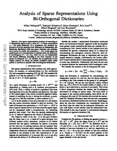
2.2. 3D shearlet representations A 3D shearlet system is obtained by combining three function systems associated with the pyramidal regions { } { } P1 = (ξ1 , ξ2 , ξ3 ) ∈ R3 : | ξξ12 | ≤ 1, | ξξ31 | ≤ 1 , P2 = (ξ1 , ξ2 , ξ3 ) ∈ R3 : | ξξ21 | < 1, | ξξ32 | ≤ 1 , } { ξ2 ξ1 3 and P3 = (ξ1 , ξ2 , ξ3 ) ∈ R : | ξ3 | < 1, | ξ3 | < 1 , b 3 is partitioned (see Fig. 1). To define such systems, let ϕ be a C ∞ in which the Fourier space R 1 1 , 16 ] and ϕˆ = 0 outside the interval [− 18 , 18 ]. univariate function such that 0 ≤ ϕˆ ≤ 1, ϕˆ = 1 on [− 16 b 3 , define That is, ϕ is the scaling function of a Meyer wavelet. For ξ = (ξ1 , ξ2 , ξ3 ) ∈ R ˆ 1 ) ϕ(ξ ˆ 2 ) ϕ(ξ ˆ 3) b b 1 , ξ2 , ξ3 ) = ϕ(ξ Φ(ξ) = Φ(ξ √ and let W (ξ) =
(2.3)
b 2 (2−2 ξ) − Φ b 2 (ξ). It follows that Φ b 2 (ξ) + Φ
∑
W 2 (2−2j ξ) = 1 for ξ ∈ R3 .
(2.4)
j≥0
Note that each function Wj = W (2−2j ·), j ≥ 0, is supported inside the Cartesian corona b 3, [−22j−1 , 22j−1 ]3 \ [−22j−4 , 22j−4 ]3 ⊂ R b 3 . Next, let V ∈ C ∞ (R) be such that and the functions Wj2 , j ≥ 0, produce a smooth tiling of R V (0) = 1, V (n) (0) = 0, for any n ≥ 1, suppV ⊂ [−1, 1] and |V (u − 1)|2 + |V (u)|2 + |V (u + 1)|2 = 1 5
for |u| ≤ 1.
(2.5)
G. Easley, D. Labate and P. Negi
ξ3
40
3D data denoising using combined sparse dictionaries
ξ3
40
ξ3
40
30
30 20
20
ξ1
ξ2
0
10
−20 −40 40 40
20
20 0
−20
−40
−40
10
−10
−20
−20
−30
−30
−40
ξ1
ξ2
0
−10
−40 40
0 −20
20
ξ1
ξ2
0
20
0
−20
−40
−40
−20
0
20
40
40 40
20 20
0 0
−20
−20 −40
−40
Figure 1: From left to right, the figure illustrates the pyramidal regions P1 , P2 and P3 in the b 3. frequency space R It was shown in [18] that there are several examples of functions V satisfying these properties. For d = 1, 2, 3, ℓ = (ℓ1 , ℓ2 ) ∈ Z2 , the 3D shearlet systems associated with the pyramidal regions Pd are defined as the collections (d)
{ψj,ℓ,k : j ≥ 0, −2j ≤ ℓ1 , ℓ2 ≤ 2j , k ∈ Z3 }, where
(2.6) −j
[−ℓ]
(d) [−ℓ] 2πiξA(d) B(d) k , ψˆj,ℓ,k (ξ) = | det A(d) |−j/2 W (2−2j ξ) F(d) (ξA−j (d) B(d) ) e
(2.7)
F(1) (ξ1 , ξ2 , ξ3 ) = V ( ξξ12 )V ( ξξ31 ), F(2) (ξ1 , ξ2 , ξ3 ) = V ( ξξ12 )V ( ξξ32 ), F(3) (ξ1 , ξ2 , ξ3 ) = V ( ξξ31 )V ( ξξ23 ), the anisotropic dilation matrices A(d) are given by 2 0 0 2 0 0 4 0 0 A(1) = 0 2 0 , A(2) = 0 4 0 , A(3) = 0 2 0 , 0 0 4 0 0 2 0 0 2 and the shear matrices are defined by 1 ℓ1 ℓ2 1 0 0 1 0 0 [ℓ] [ℓ] [ℓ] B(1) = 0 1 0 , B(2) = ℓ1 1 ℓ2 , B(3) = 0 1 0 . 0 0 1 0 0 1 ℓ1 ℓ2 1 Due to the assumptions on W and v, the elements of the system of shearlets (2.6) are well localized (1) and bandlimited. In particular, the shearlets ψˆj,ℓ,k (ξ) can be written more explicitly as ) ( ξ ) ( ξ −j [−ℓ1 ,−ℓ2 ] (1) k j 3 −2j −2j j 2 ˆ ψj,ℓ1 ,ℓ2 ,k (ξ) = 2 W (2 ξ) V 2 − ℓ1 V 2 − ℓ2 e2πiξA(1) B(1) , ξ1 ξ1
(2.8)
showing that their supports are contained inside the trapezoidal regions {(ξ1 , ξ2 , ξ3 ) : ξ1 ∈ [−22j−1 , −22j−4 ] ∪ [22j−4 , 22j−1 ], | 6
ξ3 ξ2 − ℓ1 2−j | ≤ 2−j , | − ℓ2 2−j | ≤ 2−j }. ξ1 ξ1
G. Easley, D. Labate and P. Negi
3D data denoising using combined sparse dictionaries
This expression shows that these support regions become increasingly more elongated at fine scales, due to the action of the anisotropic dilation matrices Aj(1) , with the orientations of these regions controlled by the shearing parameters ℓ1 , ℓ2 . A typical support region is illustrated in Fig. 2. Similar properties hold for the elements associated with the regions P2 and P3 .
40
ξ3
20
ξ2
0
ξ1
−20 −40 40 20 0 −20 −40 −40
0
−20
20
40
Figure 2: Frequency support of a representative shearlet function ψj,ℓ,k , inside the pyramidal region P1 . The orientation of the support region is controlled by ℓ = (ℓ1 , ℓ2 ); its shape is becoming more elongated as j increases (j = 4 in this plot). A Parseval frame of shearlets for L2 (R3 ) is obtained by combining the systems of shearlets associated with the 3 pyramidal regions Pd , d = 1, 2, 3, together with a coarse scale system, which will take care of the low frequency region. Namely, we define the 3D shearlet systems for L2 (R3 ) as the collections { }∪{ } ψe−1,k : k ∈ Z3 ψej,ℓ,k,d : j ≥ 0, |ℓ1 | < 2j , |ℓ2 | ≤ 2j , k ∈ Z3 , d = 1, 2, 3 } ∪{ j 3 e ψj,ℓ,k : j ≥ 0, ℓ1 , ℓ2 = ±2 , k ∈ Z (2.9) consisting of: • the coarse-scale shearlets {ψe−1,k = Φ(· − k) : k ∈ Z3 }, where Φ is given by (2.3); • the interior shearlets {ψej,ℓ,k,d = ψj,ℓ,k : j ≥ 0, |ℓ1 ||ℓ2 | < 2j , k ∈ Z3 , d = 1, 2, 3}, where (d)
(d)
ψj,ℓ,k are given by (2.7); • the boundary shearlets {ψej,ℓ,k,d : j ≥ 0, |ℓ1 | ≤ 2j , ℓ2 = ±2j , k ∈ Z3 , d = 1, 2, 3}, obtained (1) (2) (3) by appropriately joining together ψj,ℓ,k , ψj,ℓ,k and ψj,ℓ,k , for ℓ1 , ℓ2 = ±2j (see [20, 21] for details). Note that these functions are band-limited and smooth in the Fourier domain.
7
G. Easley, D. Labate and P. Negi
3D data denoising using combined sparse dictionaries
For simplicity of notation we will write the 3D shearlet system (2.9) as {ψeµ , µ ∈ M},
(2.10)
where M = MC ∪ MI ∪ MB are the indices associated with the coarse-scale shearlets, the interior shearlets and the boundary shearlets, as given by (2.9). Hence, we have the following result which uses properties (2.4)-(2.5) and whose proof is found in [20]. Theorem 1. The 3D system of shearlets (2.10) is a Parseval frame of L2 (R3 ). That is: ∑ |⟨f, ψeµ ⟩|2 = ∥f ∥2 , ∀f ∈ L2 (R3 ). µ∈M
2.3. Optimally sparse 3D approximations using shearlets One of the most important results about shearlet representations is that the 3D Parseval frame of shearlets {ψeµ , µ ∈ M} achieve an essentially optimal approximation rate for piecewise smooth functions of three variables [19, 20]. More precisely, let M be the class of indicator functions of sets B ⊂ [0, 1]3 whose boundary is C 2 regular and let Cc2 ([0, 1]3 ) be the collection of twice differentiable functions supported inside [0, 1]3 . Hence, we define the set E 2 ([0, 1]3 ) of functions which are C 2 away from a C 2 surface as the collection of functions of the form f = f0 + f1 χ B , ∑ where f0 , f1 ∈ Cc2 ([0, 1]3 ), B ∈ M and ∥f ∥C 2 = |α|≤2 ∥Dα f ∥∞ ≤ 1. This is a reasonable model for piecewise smooth 3D data, extending the similar 2D model of cartoon-like images introduced by Donoho in [9]. We have the following result [20]. Theorem 2. Let f ∈ E 2 and fNS be the N –term approximation of f obtained from the N largest coefficients of its shearlet expansion, namely ∑ ⟨f, ψeµ ⟩ ψeµ , fNS = µ∈IN
where IN ⊂ M is the set of indices corresponding to the N largest entries of the sequence {|sµ (f )| = |⟨f, ψeµ ⟩|2 : µ ∈ M }. Then ∥f − fNS ∥22 ≤ C N −1 (log N )2 . Up to the log-like factor, Theorem 2 yields the optimal approximation rate, outperforming wavelet approximations which only achieve an approximation rate of order O(N −1/2 ). Shearlets are the only system known to satisfy such approximation properties. As a consequence of this result, it follows from the observation of Section 1. that, for the solution of the denoising problem (1.1), under the assumption that f ∈ E 2 , a shearlets-based shrinkage estimator achieves the 2 essentially optimal rate O(σ), in contrast to wavelets which only achieve the rate O(σ 3 ). An implementation of the shearlet-based estimator for 3D data denoising has been derived by two of the authors in [30], where several numerical demonstrations have shown that the performance of this algorithm is very competitive, as compared to other advanced multiscale methods including 3D curvelets and surfacelets. 8
G. Easley, D. Labate and P. Negi
3D data denoising using combined sparse dictionaries
3. 3D data denoising using combined dictionaries Let us examine the denoising problem from the point of view of discrete signals. Let x ∈ RN and suppose that we want to recover x from the noisy observations (1.1). Since the signals of interest have some “structure”, adopting the point of view of sparse representations we assume that x is 3 sparse in an overcomplete dictionary, represented in a matrix form as D where D ∈ RN ×K , with K ≫ N 3 . That is, writing K ∑ x = Dα = αk d k , 3
k=1
where D = [di , . . . , dk ], dk ∈ R , we expect that “many” of the representations coefficients αk are negligible. If we want to minimize the number of non-negligible coefficients, we can set up the minimization problem N3
α ˆ = min∥α∥0
subject to ∥y − Dα∥2 ≤ σ,
(3.1)
where the ℓ0 norm3 is counting the number of nonzero entries of α = (αk ), that is, ∥(αk )∥0 = #{k : αk ̸= 0}. Since the algorithmic solution of (3.1) is NP-hard, this problem is usually modified by relaxing ℓ0 to an ℓ1 -norm, hence leading to the basis pursuit denoising (BPDN) problem [5] α ˆ = min∥α∥1
subject to ∥y − Dα∥2 ≤ σ,
(3.2)
and the estimator xˆ = Dα ˆ . There are many ways to solve this problem rather efficiently including interior point methods and gradient projections (cf. [15]). For an appropriate Lagrange multiplier λ, the solution of (3.2) is exactly the solution of the unconstrained optimization problem4 min λ∥α∥1 + α
1 ∥y − Dα∥22 . 2
(3.3)
In the special case where the analysis operator W associated with the dictionary D is unitary, then equation (1.2), with D = W T , is the unique solution of problem (3.2) or (3.3). Interestingly, in this case, the shrinkage algorithm also yields the solution of problem (3.1). We refer to Ch. 5 in [15] for further detail. When the dictionary is redundant, then the solution of minimization problem (3.2) or (3.3) is not necessarily the solution of the shrinkage method (1.2). Yet, also in this case, appropriate iterative-shrinkage algorithms have been introduced which extend the classical Donoho-Johnstone wavelet shrinkage method, such as the algorithms introduced by Starck et al. [1, 33] and the celebrated algorithm of Daubechies et al. [6]. We are interested in the situation where the data to be recovered are known to be a superposition of several components, each one having a sparse representation with respect ∑K to a certain dictionary. In this case, we model the data x to be recovered in (1.1) as x = k=1 xk and we use a dictionary built by amalgamating several subdictionaries D1 , . . . , DK such that each xk has a sparse representation in the subdictionary Dk but its representation in the subdictionaries Dl , 3 4
This is not technically a norm, but this abuse of notation is customary in the literature. This last formulation is known in statistics as penalized least square estimation problem.
9
G. Easley, D. Labate and P. Negi
3D data denoising using combined sparse dictionaries
l ̸= k, is not sparse. Specifically, in many situations it is reasonable to assume that the data contain textured components along with piecewise smooth components. Hence, we assume that x is a superposition x = xp + xt , where xp and xt are the piecewise smooth component and textured component of the data, respectively. In this setting, for the subdictionary associated with texture component of the data we can choose a local discrete cosine dictionary or an appropriate Gabor frame, which are known to be sparse for locally periodic patterns. For the piecewise smooth component of the data, we can choose a shearlet or a curvelet dictionary, which are known to be sparse for this type of data. The incoherence of the two dictionary has been verified heuristically in [32] (using DCT and curvelet dictionaries) and more recently and rigorously in [23]. Then, to solve this problem, we can set up the following the minimization problem: α ˆt, α ˆ p = min λ (∥αt ∥1 + ∥αp ∥1 ) + αt ,αp
1 ∥y − Dt αt − Dp αp ∥22 , 2
(3.4)
where Dt , Dp are the dictionary associated with the piecewise smooth component and textured component of the data, respectively.. The final estimate is then found by adding together the two components obtained by xˆp = Dp α ˆ p and xˆt = Dt α ˆ t . Note that, since the dictionaries are assumed to be tight frames, then Dp is the Moore-Penrose pseudo inverse of the analysis operator Wp associated with piecewise smooth data, i.e. Dp = Wp† and, similarly, Dt is the Moore-Penrose pseudo inverse of the analysis operator Wt associated with texture data, i.e., Dt = Wt† . For reason which will become clear below, rather than using a sparsity-based synthesis model as in (3.4), we have preferred to use a sparsity-based analysis model leading to the minimization problem 1 xˆp , xˆt = arg min λ∥Wp xp ∥1 + λ∥Wt xt ∥1 + ∥y − xp − xt ∥22 . (3.5) xp ,xt 2 The dichotomy between the synthesis and analysis models 5 is well discussed, for example, in [16]. While in the synthesis formulation signals are modeled as sparse linear combinations of dictionary atoms, the analysis formulation emphasizes the zeros in the analysis side (rather than the nonzeros), leading to better performance. In particular, one of the major advantages of using the formulation (3.5) rather than (3.5) is that it requires searching lower dimensional vectors rather than longer dimensional representation coefficient vectors. To further improve the performance, we have also included a total variation regularization term, which is effective at reducing possible ringing artefacts near the edges. This idea was proposed and validated not only in [32], bur also in earlier wavelet papers such as [26]. Thus, we finally have the optimization problem: 1 xˆp , xˆt = arg min λ∥Wp xp ∥1 + λ∥Wt xt ∥1 + γ T V (xp ) + ∥y − xp − xt ∥22 , xp ,xt 2 5
Note that the two models coincide when the dictionary is an ON basis.
10
(3.6)
G. Easley, D. Labate and P. Negi
3D data denoising using combined sparse dictionaries
where T V is the Total Variation. Once the separate estimates xˆp and xˆt are obtained as a solution of (3.6), the final estimator of x is given as xˆ = xˆp + xˆt . A fast convergent iterative shrinkage algorithm that solves (3.6) may be derived by using Separable Surrogate Functionals (SSF) (see [31] for its derivation) which can be summarized as follows. We start the algorithm by initializing k = 1 and setting x0p = 0, x0t = 0, r0 = y − x0p − x0t , and 0 λ = 12 (∥Wp y∥∞ + ∥Wt y∥∞ ) . We repeatedly update the estimate of xp and xt as ( ) 1 k † k−1 k−1 x˜p = Wp Tλk Wp r + Wp xp c ( ) xkp = H † Tγ k H x˜kp ( ) 1 † k k−1 k−1 xt = Wt Tλk , Wt r + Wt xt c where H is the undecimated Haar wavelet transform. The parameter c is chosen so that it is greater than the maximum eigenvalue of (Wp† Wp + Wt† Wt ). In this particular case, c set to 3 is heuristically found to work well. The residual is updated as rk = y − xkp − xkt . and the shrinkage parameter is updated as λk =
) 1( ∥Wp rk ∥∞ + ∥Wt rk ∥∞ . 2
The Haar shrinkage value γ k is dependent on the kth iteration since it is set to 3σxkp , where σxkp is the standard deviation of the noise estimate of x˜kp found by using a median estimator on the finest scale of the Haar wavelet coefficients. In our numerical tests, the iterations are stopped when λk becomes smaller then a chosen threshold. For this procedure, we chose this stopping threshold to be 2.1 times the estimate of the standard deviation of the noisy data.
4. Numerical experiments To validate our denosing strategy, based on the method described in the previous section, we have built and applied two different types of combined dictionaries, using in one case a combination of our new 3D shearlet transform [30] and local 3D DCT; in another case, a combination of 3D curvelets [2] and local 3D DCT. We denote these dictionary by Shear/DCT and Curv/DCT, respectively. We have run several numerical experiments for 3D data denoising using as sample data two video sequences that we refer to as Tempete and Oil painting. All these video sequences, which have been resized to 1923 can be uploaded from the website http://www.cipr.rpi.edu. For a baseline comparison, we tested the performance of the combined-dictionary denoising algorithm against: 3D discrete wavelet transform (DWT) using the “Sym4” filter; 3D curvelet transform (Curv); 3D shearlet transform (shear); the 3D Laplacian Pyramid (LP). In all these cases, the 11
G. Easley, D. Labate and P. Negi
3D data denoising using combined sparse dictionaries
(a)
(b)
Figure 3: (a) The 150th image frame of the Tempete video with an additive Gaussian noise whose standard deviation is 20. (b) The 60th image frame of the Oil painting video with an additive Gaussian noise whose standard deviation is 20. denoising algorithm is based on the standard soft thresholding, as described in Section 1.. To provide additional baseline comparisons of our combined dictionary techniques, we also expanded the comparisons to include an adaptation of our projection iterative scheme to work with the combinations of the 3D wavelet transform and the local DCT (DWT/DCT) and the 3D Laplacian Pyramid and the local DCT (LP/DCT). The results of these numerical experiments are given in Tables I and II where we used the peak signal-to-noise ratio (PSNR), measured in decibles (dB), given as P SN R = 20 log10
255N , ∥f − f˜∥F
where ∥ · ∥F is the Frobenius norm and f is the video array assumed to be of size N × N × N . The numbers in bold indicate the best performance for the given experiment. Furthermore, we included several figures extracted from the video sequences to illustrate the performance of the various denoising algorithms. Figure 3 shows representative image slices with an additive Gaussian noise incorporated. Illustrations from the Tempete and Oil painting video are reported in Figures 4 and 5, respectively. The result reported in this paper show that the new denosing algorithm based on the combination of 3D shearlet and local DCT dictionaries provide the best performance among the methods considered, which are state-of-the-art. As compared with the performance of the ‘standard’ 3D shearlet (Shear) denosing routine, this result shows the advantage of using a combined rather than a single dictionary, consistently with the general principles which are discussed above (Section 3.). Furthermore, our results show that the Shear/DCT routine performs significantly better than similar routines which use combined dictionaries of 3D curvelets and DCT or 3D wavelets and DCT. 12
G. Easley, D. Labate and P. Negi
3D data denoising using combined sparse dictionaries
The improvement with respect to wavelet-based routines is expected, since shearlets provide a sparser dictionary for piecewise smooth data, and their superior performance in denoising applications was already observed in [13, 14, 30]. For the comparison with curvelets, the difference in performance is due mostly to the different strategy used for the implementation of the discrete shearlet transform versus the discrete curvelet transform, where the first transform uses higher redundancy and highly selective directional filter. We refer to [30] for a comparison of 3D shearlets, 3D curvelets, surfacelets and other multiscale transforms in denoising applications using single sparse dictionaries. Table I: Denoising results (PSNR) using Tempete video.
σ 20 30 40
Noisy 22.14 18.62 16.12
DWT LP Shear 22.61 23.10 25.87 22.10 22.04 24.63 20.47 21.30 23.69
Curv 22.60 22.27 22.00
Shear/DCT DWT/DCT LP/DCT 27.47 24.09 24.45 25.61 22.38 22.61 24.34 21.40 21.51
Curv/DCT 25.29 23.02 21.97
Table II: Denoising results (PSNR) using Oil painting video.
σ 20 30 40
Noisy 22.14 18.62 16.12
DWT LP Shear 26.34 27.01 28.04 24.81 25.52 27.12 23.87 24.26 26.33
Curv 27.32 26.86 26.44
Shear/DCT DWT/DCT LP/DCT 31.01 27.74 28.32 29.07 26.03 26.37 27.68 24.89 25.02
Curv/DCT 27.66 25.94 24.67
In addition to testing the performance of the new denoising routines on video sequences, we have also tested the routine on a 3D scan of a neuronal network dataset that naturally contains noise due to the imaging sensor. In this case, we cannot provide a quantitative measure of the performance, but only a qualitative assessment based on appearance. Figure 6 displays the results of the various denoising methods for a particular slice of the original 1923 dataset. Acknowledgments. DL and PN acknowledge support from NSF grants DMS 1008900 and DMS 1005799. DL also acknowledges support from NHARP grant 003652-0136-2009. The authors thank W. Shain and B. Roysam for providing the biological sample data used to produce Figure 6.
References [1] J. Bobin, J.-L. Starck, M.J. Fadili, Y. Moudden, and D.L. Donoho. Morphological component analysis: an adaptive thresholding strategy, IEEE Trans. Image Process. 16(11) (2007), 2675-2681. 13
G. Easley, D. Labate and P. Negi
DWT
DWT/DCT
Shear
3D data denoising using combined sparse dictionaries
Curv
Curv/DCT
Shear/DCT
Figure 4: The denoising performance on a representative frame of the video sequence Tempete using various denoising routines when the additive Gaussian noise has σ = 20. Starting from the top left: denoised frame using 3D DWT (PSNR=22.61 dB), 3D Curv (PSNR=27.32 dB), 3D DWT/DCT (PSNR=24.09 dB), 3D Curv/DCT (PSNR=25.29 dB), 3D Shear (PSNR=25.87 dB), and 3D Shear/DCT (27.47 dB). 14
G. Easley, D. Labate and P. Negi
LP
LP/DCT
Shear
3D data denoising using combined sparse dictionaries
DWT/DCT
Curv/DCT
Shear/DCT
Figure 5: The denoising performance on a representative frame of the video sequence Oil painting using various denoising routines when the additive Gaussian noise has σ = 40. Starting from the top left: denoised frame using 3D LP (PSNR=24.26 dB), 3D DWT/DCT (PSNR=24.89 dB), 3D LP/DCT (PSNR=25.02 dB), Curv/DCT (PSNR=24.67 dB), Shear (PSNR=26.33 dB), and Shear/DCT (27.68 dB). 15
G. Easley, D. Labate and P. Negi
3D data denoising using combined sparse dictionaries
Noisy Data
DWT/DCT
LP/DCT
Curv
Curv/DCT
Shear/DCT
Figure 6: The denoising performance on a representative frame of a 3D network of astrocytes using various denoising routines. The routine based on the 3D-shearlet/DCT combined dictionaries seems to give the best visual performance. 16
G. Easley, D. Labate and P. Negi
3D data denoising using combined sparse dictionaries
[2] E. J. Cand`es, L. Demanet, D. Donoho, L. Ying. Fast discrete curvelet transforms, Multiscale Model. Simul. 5 (2006), 861–899. [3] E. J. Cand`es, D. L. Donoho. Ridgelets: the key to high dimensional intermittency? Philosophical Transactions of the Royal Society of London A, 357 (1999), 2495–2509. [4] E. J. Cand`es, D. L. Donoho. New tight frames of curvelets and optimal representations of objects with C 2 singularities, Comm. Pure Appl. Math., 57 (2004), 219–266. [5] S. S. Chen, D. L. Donoho, and M. A. Saunders. Atomic decomposition by basis pursuit, SIAM Rev. 43(1) (2001), 129-159. [6] I. Daubechies, M. Defrise, C. De Mol. An iterative thresholding algorithm for linear inverse problems with a sparsity constraint, Comm. Pure Appl. Math. 57 (2004), 1413-1457. [7] D. L. Donoho. Denoising by soft thresholding, IEEE Trans. Inf. Theory, 41(3) (1995), 613627. [8] D. L. Donoho. Sparse components of images and optimal atomic decomposition, Constr. Approx. 17(2001), 353–382. [9] D. L. Donoho. Wedgelets: nearly-minimax estimation of edges, Annals of Statistics, 27 (1999), 859–897. [10] D. L. Donoho and I. M. Johnstone. Ideal spatial adaptation by wavelet shrinkage, Biometrika 81(3) (1994), 425-455. [11] D. L. Donoho and I. M. Johnstone. Adapting to unknown smoothness via wavelet shrinkage, J. Amer. Statist. Assoc. 90 (1995), 1200-1224. [12] D. L. Donoho, I. M. Johnstone, G. Kerkyacharian, and D. Picard. Wavelet shrinkageAsymptopia, J. Roy. Statist. Soc. BMethodological 57(2) (1995), 301-337. [13] G. R. Easley, D. Labate, F. Colonna. Shearlet-based total variation diffusion for denoising, IEEE Trans. Image Proc. 18 (2) (2009), 260–268. [14] G. R. Easley, D. Labate, W. Lim. Sparse directional image representations using the discrete shearlet transform, Appl. Comput. Harmon. Anal., 25 (1) (2008), 25–46. [15] M. Elad. Sparse and Redundant Representations: From Theory to Applications in Signal and Image Processing, Springer, New York, NY, 2010. [16] M. Elad, P. Milanfar, and R. Rubinstein. Analysis Versus Synthesis in Signal Priors, Inverse Problems, 23(3) (2007), 947–968. [17] K. Guo, G. Kutyniok, D. Labate. Sparse Multidimensional Representations using Anisotropic Dilation and Shear Operators, in: Wavelets and Splines, G. Chen and M. Lai (eds.), Nashboro Press, Nashville, TN (2006), 189–201. 17
G. Easley, D. Labate and P. Negi
3D data denoising using combined sparse dictionaries
[18] K. Guo, D. Labate. Optimally Sparse Multidimensional Representation using Shearlets, SIAM J. Math. Anal., 9 (2007), 298–318 [19] K. Guo, Labate. Optimally sparse 3D approximations using shearlet representations, Electron. Res. Announc. Math. Sci. 17 (2010), 126–138. [20] K. Guo, and D. Labate. Optimally sparse representations of 3D Data with C 2 surface singularities using Parseval frames of shearlets, SIAM J Math. Anal. 44 (2012), 851–886. [21] K. Guo, and D. Labate, The Construction of Smooth Parseval Frames of Shearlets, preprint (2011). [22] X. Huo. Sparse Image Representation Via Combined Transforms, Ph.D. Thesis, Stanford University, 1999. [23] G. Kutyniok. Clustered sparsity and separation of cartoon and texture, preprint (2012). [24] D. Labate, W.-Q Lim, G. Kutyniok, and G. Weiss. Sparse multidimensional representation using shearlets, in Wavelets XI, edited by M. Papadakis, A. F. Laine, and M. A. Unser, SPIE Proc. 5914 (2005), SPIE, Bellingham, WA, 2005, 254–262. [25] Y. Lu and M. N. Do. Multidimensional directional filter banks and surfacelets, IEEE Trans. Image Process., 16(4) (2007), 918–931. [26] F. Malgouyres. Minimizing the total variation under a general convex constraint for image restoration, IEEE Trans. Signal Process. 11(12) (2002), 1450–1456. [27] S. Mallat. A Wavelet Tour of Signal Processing.Third Edition: The Sparse Way, Academic Press, San Diego, CA, 2008. [28] F. G. Meyer, A. Z. Averbuch and R. Coifman. Multi-layered image representation: Application to image compression, IEEE Trans. Image Process. 11(6) (1998), 1072–1080. [29] A. Narayanaswamy, Y. Wang, B. Roysam, 3-D image pre-processing algorithms for improved automated tracing of neuronal arbors, Neuroinformatics 9(2-3) (2011), 219–31. [30] P. S. Negi, D. Labate. 3D discrete shearlet transform and video processing, IEEE Trans. Image Process. 21(6) (2012), 944–2954. [31] V. M. Patel, G. R. Easley, R. Chellappa, Component-based restoration of speckled images, Proceedings 18th IEEE International Conference on Image Processing (ICIP), 2011. [32] J. L. Starck, M. Elad, D.L. Donoho. Image decomposition via the combination of sparse representations and a variational approach, IEEE Trans. Image Process. 14(10) (2005), 1570– 1582. [33] J. L. Starck, F. Murtagh, A. Bijaoui. Multiresolution support applied to image filtering and restoration, Graphic. Models Image Process. 57 (1995), 420–431. 18
G. Easley, D. Labate and P. Negi
3D data denoising using combined sparse dictionaries
[34] J. L. Starck, F. Murtagh, J. M. Fadili. Sparse Image and Signal Processing, Cambridge University Press, New York, NY, 2010. [35] A. Woiselle, J. L. Starck, J. M. Fadili. 3-D Data denoising and inpainting with the LowRedundancy Fast Curvelet Transform, J. Math. Imaging Vis. 39(2) (2011), 121–139.
19