Mar 14, 1993 - Graduate Research Assistant. §. Associate Professor of Mechanical Engineering, Mail Code 104-44, Caltech, Pasadena, CA. 91125. 1 ...
Determining Optimal Points of Membership with Dependent Variables∗ Kevin N. Otto† Engineering Design Research Laboratory Department of Mechanical Engineering Massachusetts Institute of Technology Andrew D. Lewis‡ Erik K. Antonsson§ Engineering Design Research Laboratory Division of Engineering and Applied Science California Institute of Technology December 4, 1991 Revised: March 14, 1993
Abstract Consider sets X and Y each with associated membership functions. Further suppose that there is a map f : X → Y. A membership may be induced on Y from the membership of X calculated using the extension principle, and the two memberships on Y may be combined to give an overall membership. The point with the highest membership in X can be determined directly or by back mapping the value with the highest membership in Y. These two ∗
Manuscript prepared for submission to Fuzzy Sets and Systems Assistant Professor of Mechanical Engineering ‡ Graduate Research Assistant § Associate Professor of Mechanical Engineering, Mail Code 104-44, Caltech, Pasadena, CA 91125 †
1
methods are equivalent under hypotheses on the membership functions and on f . An example calculation from engineering design is presented.
Keywords: Fuzzy numbers; algebra; engineering.
Introduction Consider a set X equipped with a membership function: every point x ∈ X has an associated value µ(x) ∈ [0, 1] ⊂ IR representing the degree of membership for x. Suppose that another set Y is mapped from X by a function f , and that Y itself has a membership function ν(y) ∈ [0, 1] ⊂ IR independent of those on X . Finally, consider combining all of the membership specifications µ(x) and ν ◦ f (x) into an overall membership µc (x) on X . This paper demonstrates that points in X which maximize overall membership can also be determined by another method. One can induce the membership specified for X onto Y by the extension principle. There one can find the y ∈ Y which maximize the overall membership, and then back map to X simply by looking up the values of x used in the original forward mapping to the optimal y. This is true even though the induced membership on Y involves only the membership µ, and does not consider any of the dependent set membership ν. The results, however, are the points which maximize the overall membership µc : the supremum of the combination of the membership specified both on X and Y. As motivation for this work, consider engineering design problems. In a typical engineering problem solved using imprecise variables, the imprecision can arise from the inability to specify the final precise values of the design variables (to be used in the problem model). We use the term design parameter to denote these variables which describe the engineering model, and must have precise values determined for the model to be solved. The initial lack of precision can be represented formally using fuzzy sets, and hence we have an example of a set X with a membership function. Dependent variables are those which are functionally related to the design parameters, and give indications of performance of the model. We term these variables performance parameters. These form a dependent variable space Y. There are also membership specifications, independent of those specified on X , placed on Y. Typically, all of the imprecise quantities are combined to solve the complete model; that is, select precise values for the design parameters [5]. This is calculated by maximizing the overall membership over the set of design parameters X . Examples are given in [5]. 2
However, it is usually of considerable interest to observe the design parameter membership expressed on the performance parameter space. This can be calculated using the extension principle [8], as will be discussed subsequently. Doing so allows a comparison of the membership functions specified on the design parameters with the membership functions specified on the dependent performance parameters. Discussion and examples are given in [6, 7]. However, this calculation can be computationally difficult. This paper demonstrates that this difficulty can be reduced, since the extension principle calculation will allow one to determine the final design parameter values directly, rather than through another computationally difficult search. We will show that the result of optimizing overall membership over the design parameters is the same as optimizing overall membership over the dependent performance parameters, and then back mapping the result to the design parameters by the image of the extension principle, even though this original inducement of membership does not involve the membership specified on the dependent performance parameters. This work is an extension of the idea, originally proposed independently by both Dubois [1] and Wood and Antonsson [6], of propogating memberships from independent variables to dependent variables, selecting optimal performance, and mapping back the membership level so as to determine the optimal parameters. We extend these ideas to general sets, rather than X ' IRN and Y ' IR, and to more general connectives than min. We consider problems which have possibly more than one optimal solution. Further, we consider independent membership specifications ν on Y, not considered in either of these previous works.
1
Definitions and Notation
The results desired do not depend on any structure associated with the variables used; as such, in the following sections, we will be working with general sets and membership functions. Thus 1.1 Definition: A membership function on a set X is a function µ : X → II = [0, 1] ⊂ IR. We are also interested in membership induced on a set from the membership on another set. This is typically done via a map between the sets as in Zadeh [8], see [2, 3] for a review. 1.2 Definition: Let X and Y be sets and let f : X → Y be a function. The induced membership on Y is νf (y) = sup{µ(x) | x ∈ X , f (x) = y}
3
We adopt the convention that νf (y) = 0 if f −1 (y) = ∅. Note that the induced membership function need not be continuous, even if X and Y are topological spaces with continuous membership functions and f is a continuous map. Now we wish to combine the membership functions on X and Y in the following manner. Let P : II 2 → II be monotonic in its first argument. Thus, if 0 ≤ a ≤ b ≤ 1, then P(a, t) ≤ P(b, t) for all t ∈ II . In this manner we can define µc (x) = P(µ(x), ν ◦ f (x))
(1.1)
νc (y) = P(νf (y), ν(y))
(1.2)
and as membership functions on X and Y, respectively. Thus µ represents membership on the design parameters, and ν represents membership on the performance parameters. The objective is to determine the most preferred point in X ; that is, the point in X which maximizes the overall membership µc . Since µc and νc are membership functions, and hence bounded, they have finite supremum over X and Y, respectively. So we can define the following numbers in II . ||µc ||∞ = sup{µc (x) | x ∈ X } (1.3) and ||νc ||∞ = sup{νc (y) | y ∈ Y}
(1.4)
We will further assume that the sets
and
X ∗ = {x ∈ X | µc (x) = ||µc ||∞ }
(1.5)
Y ∗ = {y ∈ Y | νc (y) = ||νc ||∞ }
(1.6)
are not empty. This is true, for example, when X and Y are topological spaces, and µc and νc are continuous with compact support. However, it may be true in other cases, and we do not wish to exclude these from consideration.
2
Results
The first result we will state will form the foundation of all our results to follow. 2.1 Proposition: νc (y) = sup{µc (x) | x ∈ X , f(x) = y} Proof: We will first prove a technical lemma. 2.2 Lemma: Let Q : IR → IR be monotonic, and let g : IR → IR be any function. Then Q(sup{g(x) | x ∈ IR}) = sup{Q(g(x)) | x ∈ IR} 4
Proof: Since Q is monotonic, the expression on the right-hand side of the equality will be evaluated at the value of x, possibly ±∞, where g attains its supremum. But this is precisely what the left-hand side of the equation returns. Now we proceed with the proof of the proposition. Using 2.2 we have νc (y) = = = = =
P(νf (y), ν(y)) P(sup{µ(x) | x ∈ X , f (x) = y}, ν(y)) sup{P(µ(x), ν(y)) | x ∈ X , f (x) = y} sup{P(µ(x), ν ◦ f (x)) | x ∈ X , f (x) = y} sup{µc (x) | x ∈ X , f (x) = y}
The following lemma will be useful in the sequel. 2.3 Lemma: ||µc ||∞ = ||νc ||∞ Proof: Choose y ∈ Y ∗ so that νc (y) = ||νc ||∞ . But νc (y) = sup{µc (x) | x ∈ X , f (x) = y} ≤ ||µc ||∞ . Thus ||νc ||∞ ≤ ||µc ||∞ . Now let x ∈ X ∗ so that µc (x) = ||µc ||∞ . Then νc (f (x)) = sup{µc (x0 ) | f (x0 ) = f (x)} ≥ ||µc ||∞ . Thus ||νc ||∞ ≥ ||µc ||∞ so ||νc ||∞ must equal ||µc ||∞ . We are interested in ascertaining the peak membership values in X given those in Y. 2.4 Theorem: f(X ∗ ) ⊂ Y ∗ . Conversely, if X and Y are topological spaces, and if i) f is continuous, and has compact support, and ii) if µc is continuous when restricted to f −1 (y) for each y ∈ Y ∗ then Y ∗ ⊂ f(X ∗ ). Proof: Let x ∈ X ∗ . Then µc (x) = ||µc ||∞ . Then νc (f (x)) = sup{µc (x0 ) | f (x0 ) = f (x)} ≥ ||µc ||∞ . By 2.3 νc (f (x)) = ||νc ||∞ and so f (x) ∈ Y ∗ . Now suppose i) and ii) hold, and let y ∈ Y ∗ so that νc (y) = ||νc ||∞ . Since f is continuous, f −1 (y) is closed for each y ∈ Y ∗ (since such a y is itself closed). Thus, since f has compact support, f −1 (y) is also compact (a closed subset of a compact set is also compact). Now µc is continuous on the compact set f −1 (y) and so assumes its maximum value in the set. But, by definition, sup{µc (x) | x ∈ f −1 (y)} = ||νc ||∞ , so there is some x ∈ f −1 (y) such that µc (x) = ||νc ||∞ = ||µc ||∞ , so x ∈ X ∗ . Thus Y ∗ ⊂ f (X ∗ ). In practice, if f is continuous, it may be possible to satisfy the hypothesis of compact support simply by restriction to the domain of interest.
5
l l/3
t
w
E
W E
t
60
Section E-E
Figure 1: Design Example: Structural Frame.
3
Example: Imprecise Engineering Calculations
Consider the design of a structural frame intended to support a weight W a distance l from a wall, as shown in Figure 1. The width and thickness of the beam is w and t respectively. Given this configuration, a designer may have preferences for the various parameters based on geometric constraints, customer requirements, etc. For the purposes of this illustration, we shall assume that all of these design parameters are crisp, except for w and t, which the designer has given imprecise specifications for, as shown in Figure 2. Given a configuration (as shown in Figure 1), typically a designer performs calculations to rate different values of the design parameters. In this example, a typical performance parameter might be maximum bending stress in the horizontal
6
bar. This is given by
σ : IR2 → IR (w, t) 7→
2l(W + ρgwtl ) 6 wt2
The designer must ensure that the bending stress is not excessive; as such, there is an imprecise specification on the dependent performance parameter space IR, as shown in Figure 2. The remaining parameter values are shown in Table 1. Now given these specifications, the designer can perform calculations, such as observing how the membership specifications made on w and t induce membership on the performance parameter space. This will be calculated using the extension principle, as reflected by Definition 1.2 (with X = IR2 , and Y = IR). The results of Section 2 apply to general combination functions. We will consider two different cases. The first is the traditional fuzzy set combination of 2 1 P(a, b) = min{a, b}. Also, we consider P(a, b) = a 3 · b 3 . First, the membership µ on X must be defined. For the two cases considered: 1 µ1 (w, t) = min{µw (w), µt (t)}, and µ2 (w, t) = (µw (w) · µt (t)) 2 . Given these definitions, the induced membership νf is defined for both combinations and is shown in Figure 3. An interesting feature of this problem is that both combination functions µ1 and µ2 result in the exact same membership νf on σ, as calculated using the extension principle, Definition 1.2. This invariance is a result of particular geometric conditions which the two combination functions and the function σ satisfy, as discussed in [4]. Having performed this calculation, the designer can then compare this induced membership with the requirement membership ν as shown in Figure 2. For example, the designer may select the optimal value of σ by combining the two membership functions with ν1,c (σ) = min{νf (σ), ν(σ)}, or, perhaps with a combination 2 1 ν2,c (σ) = νf (σ) 3 · ν(σ) 3 . These reflect two different possible combination functions, but the results of Section 2 apply to both. The results of applying the two methods are shown in Figure 4. Consider now the optimal values of σ as defined by the maximum of values of ν1,c and ν2,c . For ν1,c , the optimal value is σ1∗ = 0.298 (GP a). For ν2,c , the optimal value is σ2∗ = 0.295 (GP a). These define the most preferred values of performance. The question is what are the optimal points wi∗ and t∗i which produce these performances σi∗ , for i = 1, 2. It can be shown that the hypotheses i) and ii) of 2.4 hold. Therefore the points used in the extension principle calculation of νf (σ ∗ ) are in fact the points used to 7
Figure 2: Specified membership functions.
8
Table 1: Constant Values parameter
Value
W
20 kN
l
4m
g
9.8
ρ
7830
m s2 kg m3
Figure 3: Induced membership.
9
Figure 4: Overall membership on σ.
10
compute νc (σ ∗ ). That is, when using min as a combination, at the optimal value of performance σ1∗ = 0.298 (GP a), the points w1 = 0.07003 (m) and t1 = 0.08834 (m) were used to calculate νf (σ1∗ ). As well, when using the product as a combination, at the optimal value σ2∗ = 0.295 (GP a), the points w2 = 0.07697 (m) and t2 = 0.08471 (m) were used to calculate νf (σ2∗ ). Theorem 2.4 demonstrates that these values of wi and ti are the optimal points of overall membership µi,c , for i = 1, 2. That is, if the designer had as well calculated wi∗ and t∗i defined by µ1,c (w1∗ , t∗1 ) = sup{min{µw (w), µt (t), ν ◦ σ(w, t)} | (w, t) ∈ IR2 } or
1
µ2,c (w2∗ , t∗2 ) = sup{(µw (w) · µt (t) · ν ◦ σ(w, t)) 3 | (w, t) ∈ IR2 }
respectively (reflecting the two different combination functions νc on σ), then the resulting wi∗ = wi and t∗i = ti . Notice the key aspect of this: νf is used to backmap the optimal points in X of νc . Thus one can use the pre-image of the design parameter induced membership νf to find the optimal point of overall membership µc , even though νf does not involve the performance parameter membership specification ν.
Conclusion This paper presents an observation about membership optimization problems with dependent parameters: one can maximize membership over either the set X , or over the dependent set Y. One could compose the dependent set membership onto X and maximize overall membership over X to find the optimal point in X . Alternatively, one could induce the original set membership onto Y and maximize overall membership over Y, and then use the pre-image of the induced membership to determine the optimal point in X . This is true despite the fact that the pre-image is of the induced membership only, not the pre-image of the overall membership. This fact is useful, since in imprecise engineering design, it is very beneficial to observe the induced membership of the design parameters on the performance parameter space, to observe the performance achievable in the model. This technique is superior to others, since it presents visual information to the designer about the model. An optimization routine will produce a (hopefully globally optimal) solution, but it presents no real information about critical aspects in the problem. If this first design process is adopted, it is useful to know the induced membership pre-image of the optimal performance value is the optimal membership point, since this eliminates the need for a subsequent search. 11
Acknowledgments This material is based upon work supported, in part, by The National Science Foundation under a Presidential Young Investigator Award, Grant No. DMC-8552695. At the time of this research Dr. Otto was an AT&T-Bell Laboratories Ph.D. scholar at Caltech, sponsored by the AT&T foundation. Any opinions, findings, conclusions or recommendations expressed in this publication are those of the authors and do not necessarily reflect the views of the sponsors.
References [1] D. Dubois, An application of fuzzy arithmetic to the optimization of industrial machining processes, Mathematical Modelling 9 (1987) 461–475. [2] D. Dubois and H. Prade, Fuzzy Sets and Systems: Theory and Applications (Academic Press, New York, 1980). [3] A. Kaufmann and M. M. Gupta, Introduction to Fuzzy Arithmetic: Theory and Applications (Electrical/Computer Science and Engineering Series, Van Nostrand Reinhold Company, New York, 1985). [4] K. Otto, A. Lewis, and E. Antonsson, Approximating α-cuts with the Vertex Method, Fuzzy Sets and Systems 55 (1993) 43–50. (Submitted for review. EDRL Technical Report 91j.) [5] K. N. Otto and E. K. Antonsson, Trade-Off Strategies in Engineering Design, Research in Engineering Design 3 (1991) 87–104. [6] K. L. Wood and E. K. Antonsson, Computations with Imprecise Parameters in Engineering Design: Background and Theory, ASME Journal of Mechanisms, Transmissions, and Automation in Design 111 (1989) 616–625. [7] K. L. Wood, K. N. Otto, and E. K. Antonsson, Engineering Design Calculations with Fuzzy Parameters, Fuzzy Sets and Systems 52 (1992) 1–20. [8] L. A. Zadeh, Fuzzy sets, Information and Control 8 (1965) 338–353.
12