ABSTRACT. Troubleshooting (TS) in UMTS networks are basic management tasks required to guarantee efficient usage of the network infrastructure. This paper ...
The 17th Annual IEEE International Symposium on Personal, Indoor and Mobile Radio Communications (PIMRC'06)
A BAYESIAN APPROACH FOR AUTOMATED TROUBLESHOOTING FOR UMTS NETWORKS Rana Khanafer(1), Lars Moltsen(2), Hervé Dubreil(1), Zwi Altman(1), and Raquel Barco(3) (2) (3) France Telecom R&D Moltsen Intelligent Software University of Malaga 38 rue du Général-Leclerc, Niels Jernes Vej 10 E.T.S.I.Telecomunicación Issy les Moulineaux 9220 Aalborg 29071 Málaga France Denmark Spain
(1)
ABSTRACT Troubleshooting (TS) in UMTS networks are basic management tasks required to guarantee efficient usage of the network infrastructure. This paper presents a methodology for automating TS tasks based on Bayesian Networks (BN). In a first learning phase, data relating symptoms and alarms to faults in the network is extracted and used to create the TS model. In a second phase, symptoms and alarms are used to identify faults with the highest probabilities. A TS case study using a dynamic system simulator illustrates the effectiveness of the proposed approach. I.
INTRODUCTION
Throughout Europe, UMTS network operators are introducing the first high bit rate data and multi-media services. To fully exploit the newly deployed expensive infrastructure, the operators need to conduct different management tasks, such as setting antenna, system and Radio Resource Management (RRM) parameters; carrying out optimization tasks; and carefully performing diagnosis and troubleshooting (TS). Diagnosis and TS are particularly complex in the first stage of life of the network, when the accessible list of Key Performance Indicators (KPI) in the Operation Management Centre (OMC) is still incomplete, and the operator lacks experience in the new radio access technology. The term troubleshooting refers to the following three steps: fault detection, cause diagnosis (i.e. identification of the cause of the problems from KPIs and alarms) and the solution deployment, namely fixing the problem. A cause could be a hardware failure, like a broken base-band card in a node B, or a bad parameter value, i.e. transmission power, antenna tilt or a control parameter such as RRM parameter. The term symptom refers to quality indicators, i.e. quality of service (QoS) perceived by the user or performance indicators characterizing the network functioning. Alarms can be triggered when there is material failure or when certain indicators exceed some thresholds. There are tens of parameters and possible hardware failures that could deteriorate the network performance and cause alarms. Furthermore, one fault could often trigger a series of alarms. In this context, in order to achieve a conclusive diagnosis, not only alarms should be taken into account, but also performance indicators.
This work has been carried out in the framework of the EUREKA CELTIC Gandalf project. 1-4244-0330-8/06/$20.002006 IEEE
The purpose of this paper is to present a method for automating diagnosis and TS tasks in UMTS networks using Bayesian Networks (BN). BN is a knowledge based method, often referred to as a Bayesian cognitive approach, that learns how to build a model from data. The data consists of the cumulative TS experience, namely the list of observed symptoms and alarms with the corresponding faults that have been inserted by the radio expert into a database. The BN uses the data to create a statistics based mathematical model which relates symptoms to causes of faults. The quality of the model improves with the volume of data in the database. Once the model has been created, a new problem can be treated by feeding observations of alarms and symptoms into the BN which in turns will compute probabilities for all faults. This process can be seen as statistical clustering. BNs have been successfully applied to diagnosis and TS for GSM networks [1-2]. The present work aims at adapting the TS model to UMTS networks and at accounting for the specific characteristics of this radio access technology, such as the interference limited system and the strong coupling between adjacent base stations (BS) [4]. Data from the network for TS is ‘expensive’ and requires precious time of radio experts to construct a significant database. In the present work a semi-dynamic network simulator developed in France Telecom R&D [6] is utilized for the TS task. The simulator can be used to study a sub-set of problems that can occur in a real network: problems related to antenna and system parameters (i.e. common channel power, or maximum BS transmitted power), and to different RRM functionalities such as admission and congestion control and mobility. The simulator allows to generate a large amount of ‘cheap’ data to adapt and fine tune the TS model, and to assess the amount of data necessary for accurate TS. Particular attention is given to identifying the minimal set of KPIs or symptoms that should be considered in the TS process, and the impact of coupling effect between a base station and its neighbours in the model. This work is carried out within the European CELTIC Gandalf project. The project focuses on automating management tasks in heterogeneous radio access networks: monitoring, diagnosis and TS, (off-line) optimization and auto-tuning. The application of the TS model to a real network will be carried out in a second phase of the project. The paper is organized as follows. Section 2 presents the mathematical framework for TS. The adaptation of the TS model for UMTS networks is described in Section 3. The tool architecture and the learning process are presented in section 4. Numerical results are given in Section 5, followed by concluding remarks in Section 6.
The 17th Annual IEEE International Symposium on Personal, Indoor and Mobile Radio Communications (PIMRC'06)
Throughout this work, the terms node B, base station and sector can be interchanged and have the same meaning. II.
MATHEMATICAL FRAMEWORK
III. DIAGNOSIS IMPLEMENTATION FOR UMTS
Denote by Ci a cause for bad functioning in the network; by Sj a symptom that can contribute to assessing the network quality; and by E a set of N symptoms {Sj}. The diagnosis consists of identifying the causes with the highest probabilities given a set of symptoms. This process can be seen as a classification process in which each class corresponds to a given cause. Using Bayes' rule, one can calculate the probability for the cause Ci to occur given the set of observed symptoms E: P (Ci E ) =
P(Ci )P (E Ci )
(1)
P (E )
P (Ci E ) is known as the posterior (conditional) density
function and P(Ci ) as the prior density function. For a fixed
Ci , P (E Ci ) is known as the likelihood function or distribution. Typically, certain conditions on the diagnosed network are known a priori, such as the type of services provided, the number of frequencies used by the base station, or any other a priori knowledge. We denote the set of conditions by D. Adding the set D to (1) gives
(
)
P Ci E , D =
(
)(
P Ci D P E Ci P (E )
)
(2)
It is assumed in (2) that the symptoms are independent of the conditions. When this assumption is not verified, the conditions should be added to the likelihood distribution and to the P(E) term. Calculating the joint likelihood distribution P (E Ci ) is difficult and impractical. We therefore utilise the Naïve Bayesian Network, which makes the assumption that symptoms given the causes are independent. With this assumption, one only needs to specify the likelihood distribution of each symptom, P S j Ci , separately. This
(
)
assumption is an approximation, particularly in WCDMA networks, however the Naïve Bayesian classifier remains efficient even with significant dependencies between the symptoms [2, 5]. Hence, the classification in the diagnosis process will be performed using the approximation:
(
)
P Ci E , D =
(
P Ci D
N
)∏ P(S j Ci ) j =1
P (E )
probabilities in (3) are learned from the observed values calculated by the simulator when faults are introduced.
(3)
In the present work, the model will be tested in a network simulator. In both learning and exploitation phases, the causes for dysfunctions (faults) are introduced, hence the prior density of the faults, P (Ci D ) , depends on how often the faults are inserted into the simulator. The remaining
The first step in developing a diagnosis and TS model is to determine the type of causes of dysfunctions that could occur, and the associated symptoms. One can benefit from the experience of TS in GSM networks, however the specificity of UMTS networks must be taken into account. For example, in previous works on GSM TS, coverage and interference have been included in the list of possible causes for faults and alarms [1-2]. In WCDMA networks, coverage, interference or cell overload are inter-related via the interference and cannot be separated. Hence a higher level of details for the causes is required. A. Causes Two types of causes are considered: hardware problems and bad parameter values that result in poor quality indicator and possible alarms. A parameter value could be too big or too small (with respect to an optimal value), denoted respectively as Par+ and Par-. The faults considered by the simulator are the following: Channel element breakdown. This cause is a hardware problem. One or several channel elements in the node B could be out of service. Pilot power: Pilot power too high, Pilot+, will extend too much the service zone of the node B that will become overloaded. Conversely, a too low pilot power, Pilot-, will decrease too much the cell extent, reduce its load and will push traffic to neighbouring cells. Antenna tilt: Problems related to antenna tilt can be easily introduced in a system simulator. As in the pilot case, tilt+/impact the cell extent, its load and that of its neighbours. Uptilted antenna will create interference in neighbouring cells and will deteriorate their performance, whereas down tilted antennas will reduce the cell range and may cause coverage holes. Mobility parameters: Mobility parameters are of particular importance in mobile networks. We consider here parameters of hysteresis events 1A and 1B, or add- and drop-windows respectively for soft handover. Add-window defines the threshold for adding a new link to the active set of a mobile and the drop-window defines the threshold for removing an existing link. For simplicity of notation, denote by RRM_MD+ and RRM_MD- add- and drop-window parameters with too high and too low values respectively. Add- and drop-windows of a given cell impact the creation and suppression of links of its neighbouring cells. In other words, poor quality indicators and alarms in one cell could be triggered by a fault in another cell. Hence, one needs to keep track of certain symptoms of a base station and its neighbours, making the troubleshooting problem more complex. In a similar manner, one could consider other RRM parameters such as admission and congestion control parameters.
The 17th Annual IEEE International Symposium on Personal, Indoor and Mobile Radio Communications (PIMRC'06)
B. Symptoms Symptoms are quality indicators or KPIs that are used to monitor quality of service perceived by the user and the network performance. When a KPI value exceeds a predetermined threshold an alarm can be triggered. The following symptoms are considered: o
Blocked call rate
o
Dropped call rate
o
Macrodiversity (MD)-blocking rate. If a request to establish a new (additional) link with a base station is denied, it is considered as a macrodiversity blocking. The ratio between the number of macrodiversity blockings and the total number of requests to establish additional links defines the MD blocking rate. In the present study, the MD blocking rate will be calculated for a base station as the average rate of all the mobiles having this station as best server.
o
Capacity / throughput. For real time (RT) traffic, capacity is given in terms of number of mobiles per service. For non real time (NRT) traffic, the throughput is utilized.
o
Ping-pong: The ping-pong KPI is calculated here as the frequency of active set updates. Another definition that is often used is the number of link establishments per time unit for each mobile station.
As explained above, for certain causes such as mobility parameters, symptoms of neighbouring cells are necessary to identify alarms. IV. ARCHITECTURE AND LEARNING PROCESS In this work, the Naïve-Bayesian model is considered (see Section 2) [1-2]. The model requires the following qualitative elements: o o o
A list of faults (causes) A list of KPIs (symptoms) A list of statistical relations between a fault and a set of KPIs
To perform the classification, the Bayesian network utilizes the following statistical input: o
o
o
Prior distributions: the probability distributions of the faults. For each KPI, the probability distribution of the KPI in the absence of faults (normal conditions). The likelihood distribution: The conditional distribution of each KPI assuming a fault. This distribution models the strength of fault-KPI relation.
The probability distributions are derived from histograms of the KPIs. Since the amount of data is limited, the KPI is divided into states (intervals), which introduce some discretization inaccuracies. These inaccuracies can be minimized by using continuous representation of the KPIs such as beta distribution functions that can be fitted to the data [2].
The troubleshooting tool architecture is depicted in Figure 1. The learning step of the troubleshooting model is performed from the “normal” and “faulty” data. The former corresponds to symptom (KPI) statistics, including possible cases of alarms when no faults are present. The latter corresponds to symptom statistics in the presence of faults.
Diagnoses
Test Data
Odyssee Simulator
TheCure
Knowledge Builder Learner Module
ADFF (XML)
Editor Module “Normal” Data
“Faulty” Data
Figure 1: Bayesian troubleshooting tool architecture. The toolset in Figure 1 consists of: o o o
The Odyssee UMTS network simulator for generating data (developed by France Telecom R&D) The Knowledge Builder for editing troubleshooting models (developed by Moltsen Intelligent Software) TheCure for computing diagnoses (developed by Moltsen Intelligent Software)
The Learner module receives the statistical distribution input data (produced by the UMTS simulator) and creates a model, which is then stored in ADFF format (ADFF is an XML language for specifying diagnosis models). The ADFF model can also be edited directly using the Editor module. The model can now be loaded by TheCure, which converts it into a Bayesian network. The latter produces a diagnosis for each case introduced in a test database. A test data case consists of KPIs from base stations that have alarms, with or without the presence of faults. From the score of the fault identification one can deduce the efficiency of the troubleshooting process. V. RESULTS Consider a UMTS sub-network with 13 tri-sectorial sites, namely with 39 base stations in a dense urban environment. The network performance is assessed using a semi-dynamic UMTS simulator. The simulator performs correlated snapshots with time interval chosen to be one second [6]. Seven faults have been considered: CE (broken channel elements); RRM_MD+ and RRM_MD- (corresponding to addand drop-window parameter values, which are too high and too small respectively (see Section 3); Pilot+ and Pilot-; Tilt+ and Tilt-. Five symptoms (KPIs) are calculated by the simulator: Dropped call rate (DCR), blocked call rate (BCR), MD_blocking (see Section 3), DL throughput, and ping-pong indicator. For each BS, four neighbours are selected having
The 17th Annual IEEE International Symposium on Personal, Indoor and Mobile Radio Communications (PIMRC'06)
the highest traffic flux with the BS, and the average KPIs for these neighbours are calculated. Each KPI is calculated and averaged over 2000 time steps of one second. Thresholds for triggering alarms are defined for each KPI, such as 2% for MD-blocking. When no a priori target value for an alarm threshold of a given KPI is known, one can use the KPI value corresponding to a given percentile, such as the 90th percentile of the histogram of all the base stations in the network in normal conditions: P (KPI i < threshold no _ fault ) ≈ 0.9
adjacent sectors may be dropped. Table II shows the statistics fed into the knowledge builder. Table I. Statistics for normal and faulty sectors in the case of excess of pilot power problem. DCR
(Pilot+ problem) [0, 0.005)
0.96
0.033
[0.005, 0.01)
0.032
0.13
[0.01, 1]
0.008
0.837
(4)
A. Normal statistics As a first step, "normal statistics" are calculated for the network without introducing faults (normal condition). One simulation has been carried out and for each KPI, the computed values are stored from each of the 39 sectors.
Figure 2 compares the dropped call rate histograms for the normal and faulty sectors in the case of a too high pilot value of 38 dBm (33 dBm has been considered as a normal value). One can see a shift to the right of the Pilot+ histogram indicating quality degradation. The DCR symptom has been divided into three states, “normal” [0.0, 0.005), “high” [0.005, 0.01) and “very high” [0.01, 1]. The resulting statistics is summarized in Table I. It is used by the BN to perform statistical clustering.
35
Normal case
30
Broken CE case
25 20 15 10 5 0 0
35
Normal case
30
Pilot+ case
20 15 10 5 0 0,02
0,04
0,06
0,04
0,06
0,08
Figure 3: Dropped call rate histograms for non-faulty (black) and faulty (white) sectors due to broken CE.
Table II. Statistics for normal and faulty sectors in the case of sectors with broken channel elements. Normal case
Faulty sectors (CE problem)
25
0
0,02
Dropped Call Rate
DCR
40
Number of sectors
40
Number of sectors
B. Faulty statistics Statistics for base stations with faults have been calculated as follows. Faults have been introduced to 5 of the 39 sectors. Eight simulations for each fault have been performed, resulting in 40 data points per fault. It is noted that due to traffic variations, the same faulty base station can be used in different simulations to generate data.
Faulty sectors
Normal case
0,08
Dropped Call Rate
Figure 2: Dropped call rate histograms for non-faulty (black) and faulty (white) sectors due to excess of pilot power. Figure 3 compares the dropped call rate histograms for the normal and faulty sectors in the case of broken channel elements (CE). 30 CEs have been allocated to a faulty site, namely 10 CE per sector. The histogram for the faulty sectors is shifted to the right, with some sectors having very high dropping rates. Mobiles moving between two faulty co-site
[0,0.005)
0.96
0.374
[0.005, 0.01)
0.032
0.008
[0.01, 1]
0.008
0.618
After feeding the knowledge builder with KPI data for both the normal and faulty cases, we can proceed and test the efficiency of the BN model. To this end, a series of simulations has been performed including faulty and nonfaulty base stations. Each time an alarm has been triggered, the KPIs of the corresponding sector and its neighbours have been introduced into the BN (TheCure in Fig. 1) that performed troubleshooting. Ten faults of each type (CE, RRM_MD+, RRM_MD-, Pilot+, Pilot-, Tilt+, and Tilt-) have been introduced to different sectors, and the total network has been evaluated in a series of 14 simulations (five faults have been introduced in each simulation). 57 among the 70 faults have been correctly diagnosed by the BN, namely the highest probability has been attributed to the correct fault. In seven among the remaining
The 17th Annual IEEE International Symposium on Personal, Indoor and Mobile Radio Communications (PIMRC'06)
thirteen cases, the correct diagnosis has been identified with the second highest probability. A series of simulations has been carried out without any faulty base station. 42 base stations have triggered an alarm. The BN has identified 18 of them as normal sectors without faults and 13 sectors as faulty but with normal second diagnosed state. The first results are very encouraging, and further work will be invested to improve the TS process in the case of false alarms, before testing the model on data from real networks. VI. CONCLUSIONS This paper has presented a methodology for automating diagnosis and troubleshooting (TS) tasks using Bayesian Networks (BN). The BN is built from a TS model, learned from data comprising alarms, symptoms and different known faults. The application has been tested using data generated by a UMTS dynamic system simulator. Initial results of BN based troubleshooting are particularly promising: most of the faults (81%) that have generated alarms have been correctly detected, whereas 73% of the alarms triggered in the absence of faults have been correctly identified in one of the first two diagnosed states. The proposed methodology allows automating UMTS troubleshooting thus rendering it more efficient. Further work is currently invested to improve the detection of false alarms by identifying the (minimal) relevant set of symptoms related to each fault and by assessing the amount of data required. The next phase of this work will focus on TS using data from a real network. REFERENCES [1] R. Barco, R. Guerrero, G. Hylander, L. Nielsen, M. Partanen and S. Patel, "Automated troubleshooting of mobile networks using Bayesian networks", in Proceedings of the IASTED International Conference, Sept. 9-12, 2002, Malaga, Spain. [2] R. Barco, V. Wille and L. Diez, "System for automated diagnosis in cellular networks based on performance indicators", European Trans. on Telecommunications, n. 16, pp. 399-409, 2005. [3] A. Gelman, J. B. Carlin, H.S. Stern and D.B. Rubin, Bayesian Data Analysis, Chapman and Hall/CRC, US, 2004. [4] S. Ben Jamaa, H. Dubreil, Z. Altman and A. Ortega, "Quality indicator matrices and their contribution to WCDMA network design", IEEE Trans. on Vehicular Technology, vol. 54, pp. 1114-1121, May 2005. [5] F. Jensen, Bayesian Networks and decision graphs, Springer-Verlag, 2001. [6] J.M. Picard, H. Dubreil, F. Garabedian, and Z. Altman, " Dynamic control of UMTS networks by load target tuning ", IEEE International Symposium VTC 2004, Genoa, Italy, May 11-14, 2004.