Section 4 describes the bootstrap learning method in de- tail. .... Figure 6: PDF generated from the alignment of a snippet, ... segmenter with the note onset PDF.
A Bootstrap Method for Training an Accurate Audio Segmenter Ning Hu and Roger B. Dannenberg Computer Science Department Carnegie Mellon University 5000 Forbes Ave Pittsburgh, PA 15213 {ninghu,rbd}@cs.cmu.edu
ABSTRACT Supervised learning can be used to create good systems for note segmentation in audio data. However, this requires a large set of labeled training examples, and handlabeling is quite difficult and time consuming. A bootstrap approach is introduced in which audio alignment techniques are first used to find the correspondence between a symbolic music representation (such as MIDI data) and an acoustic recording. This alignment provides an initial estimate of note boundaries which can be used to train a segmenter. Once trained, the segmenter can be used to refine the initial set of note boundaries and training can be repeated. This iterative training process eliminates the need for hand-segmented audio. Tests show that this training method can improve a segmenter initially trained on synthetic data. Keywords: Bootstrap, music audio segmentation, note onset detection, audio-to-score alignment.
1
INTRODUCTION
Audio Segmentation is one of the major topics in Music Information Retrieval (MIR). Many MIR applications and systems are closely related to audio segmentation, especially those that deal with acoustic signals. Audio segmentation is sometimes the essential purpose of the application, such as dividing acoustic recordings into singing solo and accompaniment parts. Alternatively, audio segmentation can form an important module in a system, for example, detecting note onsets in the sung queries for Query-by-Humming systems. A common practice is to apply various machine learning techniques to the audio segmentation problem, and there are many satisfying results. Some of the representative machine learning models used in this area are the Hidden Markov Model (HMM) (Raphael, 1999), Neural Permission to make digital or hard copies of all or part of this work for personal or classroom use is granted without fee provided that copies are not made or distributed for profit or commercial advantage and that copies bear this notice and the full citation on the first page. c
2005 Queen Mary, University of London
Network (Marolt et al., 2002), Support Vector Machine (SVM) (Lu et al., 2001), Hierarchical Model (Kapanci and Pfeffer, 2004), etc. However, as in many other machine learning applications, audio segmentation using machine learning schemes inevitably faces a problem: getting training data is difficult and tedious. Manually segmenting each note in a five-minute piece of music can take several hours of work. Since the quantity and quality of the training data directly affects the performance of the machine learning model, many designers have no choice but to label some training data by hand. Meanwhile, the research of audio-to-score alignment has become a popular MIR topic in recent years. Linking signal and symbolic representations of music can enable many interesting applications, such as polyphonic music retrieval (Hu et al., 2003), real-time score following (Raphael, 2004), and intelligent editors (Dannenberg and Hu, 2003). In a sense, audio-to-score alignment and music audio segmentation are closely related. Both the operations are performed on acoustic features extracted from the audio, though alignment focuses on global correspondence while segmentation focuses on local changes. Given a precise alignment between the symbolic and corresponding acoustic data, desired segments can be easily extracted from audio. Even if alignment is not that precise, it still provides valuable information to music audio segmentation. Conversely, given a (precise) segmentation, alignment becomes almost trivial. This relationship between alignment and segmentation can be exploited to improve music segmentation. We propose a bootstrap method that uses automatic alignment information to help train the segmenter. The training process consists of two parts. One is an alignment process that finds the time correspondence between the symbolic and acoustic representations of a music piece. The other part is an audio segmentation process that extracts note fragments from the acoustic recording. Alignment is accomplished by matching sequences of chromagram features using Dynamic Time Warping (DTW). The segmentation model is a feed-forward neural network, with several features extracted from audio as the inputs, and a real value between 0 and 1 as the output. The alignment results help to train the segmenter iteratively. Our implementation and evaluation show that this training scheme is feasible, and that it can greatly improve the per-
223
formance of audio segmentation without manually labeling any training data. Though we need to note that the audio segmentation process discussed in this paper is aimed at detecting note onsets, this bootstrap learning scheme combined with automatic alignment can also be used for other kinds of audio segmentation. The initial purpose of this project is to aid the research of creating high-quality music synthesis by listening to acoustic examples. The synthesis approach combines a performance model that derives appropriate amplitude and frequency control signals from a musical score with an instrument model that generates sound with appropriate time-varying spectrum. In order to learn the properties of amplitude and frequency envelopes for the performance model, we need to segment individual notes from acoustic recordings and link them to corresponding score fragments. This certainly requires a audio-to-score alignment process. We previously developed a polyphonic audio alignment system and effectively deployed it in several applications (Hu et al., 2003) (Dannenberg and Hu, 2003). But we face a particular challenge when trying to use the alignment system in this case, mainly due to the special requirement imposed by the nature of instrumental sounds. For any individual note generated by a musical instrument, the attack part is perceptually very important. Furthermore, attacks are usually very short. The attack part of a typical trumpet tone lasts only about 30 milliseconds (see Figure 1). But due to limits imposed by the acoustic features used for alignment, the size of the analysis windows is usually 0.1 to 0.25 s, which is not small enough for note segmentation, especially the attack part, which can be easily overlooked. Therefore, we must pursue accurate audio alignment with a resolution of several milliseconds. Because our segmentation system is developed for music synthesis, we are mainly concerned with monophonic audio, but we believe that it should not be too difficult to extend this work to deal with polyphonic music.
Figure 1: A typical trumpet slurred note (a mezzo forte C4 from an ascending scale of slurred quarter notes), displayed in waveform along with the amplitude envelope . Attack, sustain and decay parts are indicated in the figure. The audio-to-score alignment process is closely related to that of Orio and Schwarz (2001), who also uses dynamic time warping to align polyphonic music to scores. While we use the chromagram (described in a later section), they use a measure called Peak Structure Dis-
224
tance, which is derived from the spectrum of audio and from synthetic spectra computed from score data. Another noteworthy aspect of their work is that, since they also intend to use it for music synthesis (Schwarz, 2004), they obtain accurate alignment using small (5.8 ms) analysis windows, and the average error is about 23 ms (Soulez et al., 2003), which makes it possible to directly generate training data for audio segmentation. However, this also greatly affects the efficiency of the alignment process. They report that even with optimization measures, their system is running ”2 hours for 5 minutes of music, and occupying 400MB memory”. In contrast, our system uses larger analysis windows and aligns 5 minutes of music in less than 5 minutes. Although we use larger analysis windows for alignment, we use small analysis windows (and different features) for segmentation, and this allows us to obtain high accuracy. In the following sections, we describe our system in detail. We introduce the audio-to-score alignment process in Section 2, and the segmentation model in Section 3. Section 4 describes the bootstrap learning method in detail. Section 5 evaluates the system and presents some experimental results. We conclude and summarize this paper in the last section.
2
AUDIO-TO-SCORE ALIGNMENT
2.1 The Chroma Representation As we mentioned above, the alignment is performed on two sequences of features extracted from both the symbolic and audio data. Compared with several other representations, the chroma representation is clearly a winner for this task (Hu et al., 2003). Thus our first step is to convert audio data into discrete chromagrams: sequences of chroma vectors. The chroma vector representation is a 12-element vector, where each element represents the spectral energy corresponding to one pitch class (i.e. C, C#, D, D#, etc.). To compute a chroma vector from a magnitude spectrum, we assign each bin of the FFT to the pitch class of the nearest step in the chromatic equal-tempered scale. Then, given a pitch class, we average the magnitude of the corresponding bins. This results in a 12-value chroma vector. Each chroma vector in this work represents 0.05 seconds of audio data (nonoverlapping). The symbolic data, i.e. MIDI file, is also to be converted into chromagrams. The traditional way is to synthesize the MIDI data, and then convert the synthetic audio into chromagrams. However, we have found a simple alternative that directly maps from MIDI events to chroma vectors (Hu et al., 2003). To compute the chromagram directly from MIDI data, we first associate each pitch class with an independent unit chroma vector - the chroma vector with only one element value as 1 and the rest as 0; then, where there is polyphony in the MIDI data, the unit chroma vectors are simply multiplied by the loudness factors, added and normalized. The direct mapping scheme speeds up the system by skipping the synthesis procedure, and it rarely sacrifices the alignment results. In fact, in most cases we have tried, the results are generally better when using this al-
ternative approach. Furthermore, it is positively necessary to bypass the synthesis step for this particular experiment. While rendering audio from symbolic data, the synthesizer Timidity++ (Toivonen and Izumo, 1995– 2004) always introduces small variations in time. But a later procedure needs to estimate note onsets in the acoustic recording by mapping from the MIDI file through the alignment path. And any asynchronization between the symbolic and synthetic data can greatly affect its accuracy. 2.2
Matching MIDI to Audio
After obtaining two sequences of chroma vectors from audio recording and MIDI data, we need to find the time correspondence between the two sequences such that corresponding vectors are similar. Before comparing the chroma vectors, we must first normalize the vectors, as obviously the amplitude level varies throughout the acoustic recordings and MIDI files. We experimented with different normalization methods, and normalizing the vectors to have a mean of zero and a variance of one seems to be the best one. But this can cause trouble when dealing with silence. Thus, if the average amplitude of an audio frame is lower than a predefined threshold, we define it as a silence frame, and assign each element of the corresponding chroma vector infinite. We then calculate the Euclidean distance between the vectors. The distance is zero if there is perfect agreement. Figure 2 shows a similarity matrix where the horizontal axis is a time index into the acoustic recording, and the vertical axis is a time index into the MIDI data. The intensity of each point is the distance between the corresponding vectors, where black represents a distance of zero.
to find the optimal alignment. DTW computes a path in a similarity matrix where the rows correspond to one vector sequence and columns correspond to the other. The path is a sequence of adjacent cells, and DTW finds the path with the smallest sum of distances. For DTW, each matrix cell (i,j) represents the sum of distances along the best path from (0,0) to (i,j). We use the calculation pattern shown in Figure 3 for each cell. The best path up to location (i,j) in the matrix (labeled D in the figure) depends only on the adjacent cells (A, B, and C) and the weighted distance between the vectors corresponding to row i and column j. Note that the horizontal step from C and the vertical step from B allow for the skipping of silence in either sequence. We √ also weight the distance value in the step from cell A by 2 so as not to favor the diagonal direction. This calculation pattern is the one we feel more comfortable with, but the resulting differences from various formulations of DTW (Hu and Dannenberg, 2002) are often too subtle to show a clear difference. The DTW algorithm requires a single pass through the matrix to compute the cost of the best path. Then, a backtracking step is used to identify the actual path. The time complexity of the automatic alignment is O(mn), where m and n are respectively the lengths of the two compared feature sequences. Assuming the expected optimal alignment path is along the diagonal, we can optimize the process by running DTW on just a part of the similarity matrix, which is basically a diagonal band representing the allowable range of misalignment between the two sequences. Then the time complexity can be reduced to O(max(m, n)).
12 10 D = Mi,j
MIDI (s)
8
j−1
j
i
C
D
i−1
A
B
√ A 2 = min( B + 1 × dist(i, j)) C 1
6
Figure 3: Calculation pattern for cell (i, j)
4
After computing the optimal path found by DTW, we get the time points of those note onsets in the MIDI file and map them to the acoustic recording according to the path (see Figure 4). The analysis window used for alignment is Wa = 50ms, and a smaller window actually makes the alignment worse because of the way chroma vectors are computed. Thus the alignment result is really not that accurate, considering the resolution from alignment is on the same scale as the analysis window size. Nevertheless, the alignment path still indicates roughly where the note onsets should be in the audio. In fact, the estimation of the error between the actual note onsets and the ones found by the path is similar to a Gaussian distribution. In other words, the possibility of observing an actual note onset around an estimated one given by the alignment is approx-
2 2
4 6 8 10 Acoustic Recording (s)
12
Figure 2: Similarity Matrix for the first part in the third movement of ”English Suite” composed by R. Bernard Fitzgerald. The acoustic recording is the trumpet performance by the second author. We use the Dynamic Time Warping (DTW) algorithm
225
12
the audio to be processed has the sample rate of 44.1 KHz, every analysis window contains 256 samples.
10
3.2 Segmentation Model
MIDI (s)
8 6 4 2 2
4 6 8 10 Acoustic Recording (s)
12
We use a multi-layer Neural Network as the segmentation model (see Figure 5). It is a feed-forward network that is essentially a non-linear function with a finite set of parameters. Each neuron (perceptron) is a Sigmoid unit, which is defined as f (s) = 1+e1 −s , where s is the input of the neuron, and f(s) is the output. The input units accept those features extracted from the acoustic signals. The output is a single real value ranging from 0 to 1, indicating the likelihood of being a segmentation point for the current audio frame. In other words, the output is the model’s estimate of the certainty of a note onset. When using the model to segment the audio file, an audio frame is classified as a note onset if output of the segmenter is more than 0.5.
Figure 4: The optimal alignment path is shown in white over the similarity matrix of Figure 2; the little circles on the path denote the mapping of note onsets. imately a Gaussian distribution. This is valuable information that can help to train the segmenter.
3 3.1
NOTE SEGMENTATION
Acoustic Features
Several features are extracted from the acoustic signals. The basic ones are listed below: • Logarithmic energy, distinguishing silent frames from the audio, Energy LogEng = 10log10 Energy , 0 where Energy0 = 1. • Fundamental frequency F 0. Fundamental frequency and harmonics are computed using the McAulayQuatieri Model (McAulay and Quatieri, 1986) provided by the SNDAN package (Beauchamp, 1993). • Relative strengths of first three harmonics Amplitudei , RelAmpi = Amplitude overall where i denotes which harmonic. • Relative frequency deviations of first three harmonics 0 RelDF ri = fi −i×F , fi where fi is the frequency of the ith harmonic • Zero-crossing rate (ZCR), serving as an indicator of the noisiness of the signal. Furthermore, the derivatives of those features are also included, as derivatives are good indicators of fluctuations in the audio such as note attacks or fricatives. All of those features are computed using a sliding nonoverlapping analysis window Ws with a size of 5.8 ms. If
226
Input
Layer 1
Layer 2
Output
Figure 5: Neural Network for Segmentation Neural networks offer a standard approach for supervised learning. Labeled data are required to train a network. Training is accomplished by adjusting weights within the network to minimize the expected output error. We use a conventional back-propagation learning method to train the model. We should note that the segmentation model used in this project is a typical but rather simple one, and its performance alone may not be the best among other more complicated models. The emphasis of this paper is to demonstrate that the alignment information can help train the segmenter and improve its performance, not how well the standalone segmenter performs.
4
Bootstrap Learning
After we get the estimated note onsets from the alignment path found by DTW, we create a probability density function (PDF) indicating the possibility of being an actual note onset at each time point in the acoustic recording. As shown in Figure 6, the PDF is generated by overlapping a set of Gaussian windows. Each window is centered at the estimated note onsets given by the alignment path, and has twice the size of the alignment analysis window (2 × 0.05s = 0.1s). For those points outside any Gaus-
sian window, the value is assigned to a small value slightly bigger than 0 (e.g. 0.04).
tect note boundaries in audio signals more precisely, as demonstrated in Figure 7.
5 EVALUATIONS
PDF Time (s)
Figure 6: PDF generated from the alignment of a snippet, which is a phrase of the music content in Figure 2. Then we run the following steps iteratively until either the weights in the neural network converge, or the validation error reaches its minimum so as not to overfit the data. 1. Execute segmentation process on the acoustic audio. 2. Multiply the sequence of real values v output by the segmenter with the note onset PDF. The result is a new sequence of values denoted as vnew . 3. For each estimated note onset, find a time point that has the biggest value vnew within a window Wp , and mark it as the adjusted note onset. The window is defined as follows: � � i−1 Wp (i) = [max Ti +T , T − W , i a � 2 � Ti +Ti+1 min , Ti + Wa ], 2
where Ti is the estimated onset time of the ith note in the acoustic recording given by alignment, and Wa is the size of the analysis window for alignment.
4. Use the audio frames to re-train the neural network. The adjusted note onset points are labeled as 1, and the rest are labeled as 0. Because the dataset is imbalanced as the number of positive examples is far less than the negative ones, we adjust the cost function to increase the penalty when false negatives occur. As the segmentation model has a smaller resolution than the alignment model, the trained segmenter can de-
The experimental data is the English Suite composed by R. Bernard Fitzgerald (Fitzgerald) for Bb Trumpet. It is a set of 5 English folk tunes artfully arranged into one work. Each of the 5 movements is essentially a monophonic melody, and the whole suite contains a total of 673 notes. We have several formats of this particular music piece, including the MIDI files created using a digital piano, the real acoustic recordings performed by the second author, and synthetic audio generated from the MIDI files. We run some experiments to compare two systems. One is a baseline segmenter, which is pre-trained using a different MIDI file and its synthetic data; the other is a segmenter with the bootstrap method, which has the same initial setup of the neural network as that of the baseline segmenter, but the alignment information is used to help iteratively train the segmenter. We run the baseline segmenter through all the audio files in the data set and compare its detected note onsets with the actual ones. For the segmenter with bootstrapping, we use cross-validation. In every validation pass, 4 MIDI files and the corresponding audio files are used to train the segmenter, and the remaining MIDI-audio files pair is used as the validataion set for stopping the training iterations to prevent data overfitting. This process is repeated so that the data of all 5 movements have once been used for validation, and the error measuring results on the validation sets are combined to evaluate the model performance. We calculate several values to measure the performance of the systems. Miss rate is defined as the ratio of missed ones among all the actual note onsets – an actual note onset is determined to be a missed one, when there is no detected onset within the window Wp around it; spurious rate is the ratio between spurious ones detected by the system and all the actual note onsets – spurious note onsets include those detected ones that do not correspond to any actual onset; average error and standard deviation (STD) indicate the attribute of the distance between each actual note onset and its corresponding detected one, if the note onset is neither missed or spurious. We first use the synthetic audio from MIDI files as the data set, and the experimental results are shown in Table 1. Table 1: Model Comparison on Synthetic Audio Model Baseline Segmenter Segmenter w/ Bootstrap
Miss Rate
Spurious Rate
Average Error
STD
8.8%
10.3%
21 ms
29 ms
0.0%
0.3%
10 ms
14 ms
We also try the two segmenters on the acoustic recordings. However, it is very difficult to take overall measures, as labeling all the note onsets in acoustic recordings is too time consuming. We have to randomly pick a set of 100
227
Estimated Note Onsets from Alignment Detected Note Onsets by Segmenter w/ Bootstrap
PDF Acoustic Waveform
Figure 7: Note segmentation results on the same music content as in Figure 6. Note that the note onsets detected by the segmenter with bootstrapping are not exactly the same as the ones estimated from alignment. This is best illustrated on the note boundary around 1.8 seconds. note onsets throughout the music piece (20 in each movement), and measure their results manually. The results are shown in Table 2. Table 2: Model Comparison on Real Recordings Model Baseline Segmenter Segmenter w/ Bootstrap
Miss Rate
Spurious Rate
Average Error
STD
15.0%
25.0%
35 ms
48 ms
2.0%
4.0%
8 ms
12 ms
As we can see, the baseline segmenter performs worse on the real recordings than on the synthetic data, which indicates there are indeed some differences between synthetic audio and real recordings that can affect the performance. Nevertheless, the segmenter with bootstrapping continues to perform very well on recordings of an acoustic instrument.
6 CONCLUSIONS Music segmentation is an important step in many music processing tasks, including beat tracking, tempo analysis, music transcription, and music alignment. However, segmenting music at note boundaries is rather difficult. In real recordings, the end of one note often overlaps the beginning of the next due to resonance in acoustic instruments and reverberation in the performance space. Even humans have difficulty deciding exactly where note transitions occur. One promising approach to good segmentation is machine learning. With good training data, supervised learning systems frequently outperform those created in an ad hoc fashion. Unfortunately, we do not have very good training data for music segmentation, and labeling acoustic recordings by hand is very difficult and time consuming. Our work offers a solution to the problem of obtaining good training data. We use music alignment to tell us (approximately) where to find note boundaries. This information is used to improve the segmentation, and the
228
segmentation can then be used as labeled training data to improve the segmenter. This bootstrapping process is iterated until it converges. Our tests show that segmentation can be dramatically improved using this approach. Note that while we use alignment to help train the segmenter, we tested the trained segmenters without using alignment. Of course, whenever a symbolic score is available, even more accurate segmentation should be possible by combining the segmenter with the alignment results. Machine learning is especially effective when many features must be considered. In future work, we hope to improve further on segmentation by considering many more signal features. This will require more training data, but our bootstrapping method should make this feasible. In summary, we have described a system for music segmentation that uses alignment to provide an initial set of labeled training data. A bootstrap method is used to improve both the labels and the segmenter. Segmenters trained in this manner show improved performance over a baseline segmenter that has little training. Our bootstrap approach can be generalized to incorporate additional signal features and other supervised learning algorithms. This method is already being used to segment acoustic recordings for a music synthesis application, and we believe many other applications can benefit from this new approach.
ACKNOWLEDGEMENTS This project greatly benefits from the helpful discussions and suggestions during the Computer Music group meetings held at Carnegie Mellon University. We would also like to thank Guanfeng Li for his valuable inputs and support.
References James Beauchamp. Unix workstation software for analysis, graphics, modifications, and synthesis of musical sounds. In Audio Engineering Society Preprint, number 3479. Berlin, 1993. Roger B. Dannenberg and Ning Hu. Polyphonic audio matching for score following and intelligent au-
dio editors. In Proceedings of the 2003 International Computer Music Conference, pages 27–34, Singapore, 2003. R. Bernard Fitzgerald. English suite. Transcribed for Bb Trumpet (or Cornet) and Piano. Ning Hu and Roger B. Dannenberg. A comparison of melodic database retrieval techniques using sung queries. In JCDL 2002: Proceedings of the Second ACM/IEEE-CS Joint Conference on Digital Libraries, 2002. Ning Hu, Roger B. Dannenberg, and George Tzanetakis. Polyphonic audio matching and alignment for music retrieval. In 2003 IEEE Workshop on Applications of Signal Processing to Audio and Acoustics, pages 185–188, New York, 2003. Emir Kapanci and Avi Pfeffer. A hierarchical approach to onset detection. In Proceedings of the 2004 International Computer Music Conference, pages 438–441, Orlando, 2004. Lie Lu, Stan Z. Li, and Hong Jiang Zhang. Content-based audio segmentation using support vector machines. In Proceedings of the IEEE International Conference on Multimedia and Expo (ICME 2001), pages 956–959, Tokyo, Japan, 2001. Matija Marolt, Alenka Kavcic, and Marko Privosnik. Neural networks for note onset detection in piano music. In Proceedings of the 2002 International Computer Music Conference, 2002. R.J. McAulay and Th.F. Quatieri. Speech analysis/synthesis based on a sinusoidal representation. IEEE Transactions on Acoustics, Speech, and Signal Processing, 34(4):744–754, 1986. Nicola Orio and Diemo Schwarz. Alignment of monophonic and polyphonic music to a score. In Proceedings of the 2001 International Computer Music Conference, pages 155–158, 2001. Christopher Raphael. Automatic segmentation of acoustic musical signals using hidden markov model. IEEE Transactions on Pattern Analysis and Machine Intelligence, 21(4), 1999. Christopher Raphael. A hybrid graphical model for aligning polyphonic audio with musical scores. In ISMIR 2004: Proceedings of the Fifth International Conference on Music Information Retrieval, 2004. Diemo Schwarz. Data-Driven Concatenative Sound Synthesis. PhD thesis, Universit Paris 6 - Pierre et Marie Curie, 2004. Ferr´eol Soulez, Xavier Rodet, and Diemo Schwarz. Improving polyphonic and poly-instrumental music to score alignment. In ISMIR 2003: Proceedings of the Fourth International Conference on Music Information Retrieval, pages 143–148, Baltimore, 2003. Tuukka Toivonen and Masanao Izumo. Timidity++, 1995–2004. an OpenSource MIDI to WAVE converter/player.
229