A brief introduction to mixed effects modelling and multi-model inference in ecology Xavier A. Harrison1, Lynda Donaldson2,3, Maria Eugenia Correa-Cano2, Julian Evans4,5, David N. Fisher4,6, Cecily E.D. Goodwin2, Beth S. Robinson2,7, David J. Hodgson4 and Richard Inger2,4 1
Institute of Zoology, Zoological Society of London, London, UK Environment and Sustainability Institute, University of Exeter, Penryn, UK 3 Wildfowl and Wetlands Trust, Slimbridge, Gloucestershire, UK 4 Centre for Ecology and Conservation, University of Exeter, Penryn, UK 5 Department of Biology, University of Ottawa, Ottawa, ON, Canada 6 Department of Integrative Biology, University of Guelph, Guelph, ON, Canada 7 WildTeam Conservation, Padstow, UK 2
ABSTRACT
Submitted 26 July 2017 Accepted 27 April 2018 Published 23 May 2018 Corresponding author Xavier A. Harrison,
[email protected] Academic editor Andrew Gray Additional Information and Declarations can be found on page 26 DOI 10.7717/peerj.4794 Copyright 2018 Harrison et al. Distributed under Creative Commons CC-BY 4.0
The use of linear mixed effects models (LMMs) is increasingly common in the analysis of biological data. Whilst LMMs offer a flexible approach to modelling a broad range of data types, ecological data are often complex and require complex model structures, and the fitting and interpretation of such models is not always straightforward. The ability to achieve robust biological inference requires that practitioners know how and when to apply these tools. Here, we provide a general overview of current methods for the application of LMMs to biological data, and highlight the typical pitfalls that can be encountered in the statistical modelling process. We tackle several issues regarding methods of model selection, with particular reference to the use of information theory and multi-model inference in ecology. We offer practical solutions and direct the reader to key references that provide further technical detail for those seeking a deeper understanding. This overview should serve as a widely accessible code of best practice for applying LMMs to complex biological problems and model structures, and in doing so improve the robustness of conclusions drawn from studies investigating ecological and evolutionary questions. Subjects Ecology, Evolutionary Studies, Statistics Keywords GLMM, Mixed effects models, Model selection, AIC, Multi-model inference,
Overdispersion, Model averaging, Random effects, Collinearity, Type I error
INTRODUCTION In recent years, the suite of statistical tools available to biologists and the complexity of biological data analyses have grown in tandem (Low-De´carie, Chivers & Granados, 2014; Zuur & Ieno, 2016; Kass et al., 2016). The availability of novel and sophisticated statistical techniques means we are better equipped than ever to extract signal from noisy biological data, but it remains challenging to know how to apply these tools, and which statistical technique(s) might be best suited to answering specific questions
How to cite this article Harrison et al. (2018), A brief introduction to mixed effects modelling and multi-model inference in ecology. PeerJ 6:e4794; DOI 10.7717/peerj.4794
(Kass et al., 2016). Often, simple analyses will be sufficient (Murtaugh, 2007), but more complex data structures often require more complex methods such as linear mixed effects models (LMMs) (Zuur et al., 2009), generalized additive models (Wood, Goude & Shaw, 2015) or Bayesian inference (Ellison, 2004). Both accurate parameter estimates and robust biological inference require that ecologists be aware of the pitfalls and assumptions that accompany these techniques and adjust modelling decisions accordingly (Bolker et al., 2009). Linear mixed effects models and generalized linear mixed effects models (GLMMs), have increased in popularity in the last decade (Zuur et al., 2009; Bolker et al., 2009). Both extend traditional linear models to include a combination of fixed and random effects as predictor variables. The introduction of random effects affords several non-exclusive benefits. First, biological datasets are often highly structured, containing clusters of non-independent observational units that are hierarchical in nature, and LMMs allow us to explicitly model the non-independence in such data. For example, we might measure several chicks from the same clutch, and several clutches from different females, or we might take repeated measurements of the same chick’s growth rate over time. In both cases, we might expect that measurements within a statistical unit (here, an individual, or a female’s clutch) might be more similar than measurements from different units. Explicit modelling of the random effects structure will aid correct inference about fixed effects, depending on which level of the system’s hierarchy is being manipulated. In our example, if the fixed effect varies or is manipulated at the level of the clutch, then treating multiple chicks from a single clutch as independent would represent pseudoreplication, which can be controlled carefully by using random effects. Similarly, if fixed effects vary at the level of the chick, then non-independence among clutches or mothers could also be accounted for. Random effects typically represent some grouping variable (Breslow & Clayton, 1993) and allow the estimation of variance in the response variable within and among these groups. This reduces the probability of false positives (Type I error rates) and false negatives (Type II error rates, e.g. Crawley, 2013). In addition, inferring the magnitude of variation within and among statistical clusters or hierarchical levels can be highly informative in its own right. In our bird example, understanding whether there is more variation in a focal trait among females within a population, rather than among populations, might be a central goal of the study. Linear mixed effects models are powerful yet complex tools. Software advances have made these tools accessible to the non-expert and have become relatively straightforward to fit in widely available statistical packages such as R (R Core Team, 2016). Here we focus on the implementation of LMMs in R, although the majority of the techniques covered here can also be implemented in alternative packages including SAS (SAS Institute, Cary, NC, USA) & SPSS (SPSS Inc., Chicago, IL, USA). It should be noted, however, that due to different computational methods employed by different packages there may be differences in the model outputs generated. These differences will generally be subtle and the overall inferences drawn from the model outputs should be the same.
Harrison et al. (2018), PeerJ, DOI 10.7717/peerj.4794
2/32
Despite this ease of implementation, the correct use of LMMs in the biological sciences is challenging for several reasons: (i) they make additional assumptions about the data to those made in more standard statistical techniques such as general linear models (GLMs), and these assumptions are often violated (Bolker et al., 2009); (ii) interpreting model output correctly can be challenging, especially for the variance components of random effects (Bolker et al., 2009; Zuur et al., 2009); (iii) model selection for LMMs presents a unique challenge, irrespective of model selection philosophy, because of biases in the performance of some tests (e.g. Wald tests, Akaike’s Information Criterion (AIC) comparisons) introduced by the presence of random effects (Vaida & Blanchard, 2005; Dominicus et al., 2006; Bolker et al., 2009). Collectively, these issues mean that the application of LMM techniques to biological problems can be risky and difficult for those that are unfamiliar with them. There have been several excellent papers in recent years on the use of GLMMs in biology (Bolker et al., 2009), the use of information theory (IT) and multi-model inference for studies involving LMMs (Grueber et al., 2011), best practice for data exploration (Zuur et al., 2009) and for conducting statistical analyses for complex datasets (Zuur & Ieno, 2016; Kass et al., 2016). At the interface of these excellent guides lies the theme of this paper: an updated guide for the uninitiated through the model fitting and model selection processes when using LMMs. A secondary but no less important aim of the paper is to bring together several key references on the topic of LMMs, and in doing so act as a portal into the primary literature that derives, describes and explains the complex modelling elements in more detail. We provide a best practice guide covering the full analysis pipeline, from formulating hypotheses, specifying model structure and interpreting the resulting parameter estimates. The reader can digest the entire paper, or snack on each standalone section when required. First, we discuss the advantages and disadvantages of including both fixed and random effects in models. We then address issues of model specification, and choice of error structure and/or data transformation, a topic that has seen some debate in the literature (O’Hara & Kotze, 2010; Ives, 2015). We also address methods of model selection, and discuss the relative merits and potential pitfalls of using IT, AIC and multi-model inference in ecology and evolution. At all stages, we provide recommendations for the most sensible manner to proceed in different scenarios. As with all heuristics, there may be situations where these recommendations will not be optimal, perhaps because the required analysis or data structure is particularly complex. If the researcher has concerns about the appropriateness of a particular strategy for a given situation, we recommend that they consult with a statistician who has experience in this area.
UNDERSTANDING FIXED AND RANDOM EFFECTS A key decision of the modelling process is specifying model predictors as fixed or random effects. Unfortunately, the distinction between the two is not always obvious, and is not helped by the presence of multiple, often confusing definitions in the literature (see Gelman & Hill, 2007, p. 245). Absolute rules for how to classify something as a fixed or random effect generally are not useful because that decision can change depending on Harrison et al. (2018), PeerJ, DOI 10.7717/peerj.4794
3/32
A
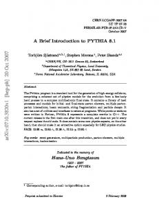
B Random Intercepts and Slopes
yi = αj + βxi
yi = αj + βjxi Dependent Variable y
Dependent Variable y
Random Intercepts
α2 α5 α1
α2 α5 α1
μgroup
μgroup
α3
α3
α4
α4
Predictor Variable x
Predictor Variable x
Figure 1 Differences between Random Intercept vs Random Slope Models. (A) A random-intercepts model where the outcome variable y is a function of predictor x, with a random intercept for group ID (coloured lines). Because all groups have been constrained to have a common slope, their regression lines are parallel. Solid lines are the regression lines fitted to the data. Dashed lines trace the regression lines back to the y intercept. Point colour corresponds to group ID of the data point. The black line represents the global mean value of the distribution of random effects. (B) A random intercepts and random slopes model, where both intercepts and slopes are permitted to vary by group. Random slope models give the model far more flexibility to fit the data, but require a lot more data to obtain accurate estimates of separate slopes for each group. Full-size DOI: 10.7717/peerj.4794/fig-1
the goals of the analysis (Gelman & Hill, 2007). We can illustrate the difference between fitting something as a fixed (M1) or a random effect (M2) using a simple example of a researcher who takes measurements of mass from 100 animals from each of five different groups (n = 500) with a goal of understanding differences among groups in mean mass. We use notation equivalent to fitting the proposed models in the statistical software R (R Core Team, 2016), with the LMMs fitted using the R package lme4 (Bates et al., 2015b): M1