A Calculus for Propagating Semantic Annotations ... - Semantic Scholar

A Calculus for Propagating Semantic Annotations through Scientific Workflow Queries? Shawn Bowers1 and Bertram Lud¨ascher1 2 1

2 UC Davis Genome Center Department of Computer Science University of California, Davis

Abstract. Scientific workflows facilitate automation, reuse, and reproducibility of scientific data management and analysis tasks. Scientific workflows are often modeled as dataflow networks, chaining together processing components (called actors) that query, transform, analyse, and visualize scientific datasets. Semantic annotations relate data and actor schemas with conceptual information from a shared ontology, to support scientific workflow design, discovery, reuse, and validation in the presence of thousands of potentially useful actors and datasets. However, the creation of semantic annotations is complex and time-consuming. We present a calculus and two inference algorithms to automatically propagate semantic annotations through workflow actors described by relational queries. Given an input annotation α and a query q, forward propagation computes an output annotation α0 ; conversely, backward propagation infers α from q and α0 .

1

Introduction

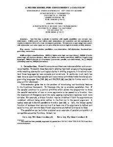
Scientific workflows aim at automating repetitive scientific data management, analysis, and visualization tasks and provide scientists with a mechanism to seamlessly “glue” together different local and/or remote applications and (web) services into complex data analysis pipelines. Fig. 1 shows a simple ecology analysis workflow for computing two biodiversity quantities called Richness and Productivity using the K EPLER scientific workflow system [17]. As can be seen from the figure, scientific workflows are often modeled as networks of computational steps (called actors) that query, transform, and analyse input datasets (here, two datasets containing measurement data) via intermediate steps and derived datasets, resulting in a number of data products (here, containing the desired Richness and Productivity information). Scientific workflow systems (e.g., K EPLER, TAVERNA [21], T RIANA [19] and many others [24]) are emerging as flexible and extensible problem-solving environments for designing, documenting, sharing, and executing scientific workflows [18]. In contrast to the use of shell scripts or spreadsheets, scientific workflows offer a versatile and controlled mechanism for automating data analysis pipelines, tracing data provenance [7,23], reproducing results, etc. As more and more workflow components and datasets become available, however, users ?

Work supported by NSF/ITR SEEK (DBI-0533368), NSF/ITR GEON (EAR-0225673), and DOE SDM (DE-FC02-01ER25486). We also thank Alin Deutsch and Alan Nash for insightful discussions on the Chase and mapping composition, respectively.

Fig. 1. Simple scientific workflow for computing species richness and productivity [9]

face the problem of selecting from thousands of possibly relevant workflow components (e.g., given as web service operations, command-line tools, functions from statistics packages such as R, or native application components), and an even larger set of possible datasets. Similarly, once candidate actor components and datasets have been identified, there is the problem of whether it is possible to “chain” them together in the desired form. Generic programming language data types (such as string or arrays of integers) do not provide any guidance as to whether it is meaningful to chain together the output(s) of one actor with the input(s) of another actor. While the use of WSDL or XML Schema types can guide workflow composition, this requires that a single common schema is adopted, which is often impractical. To at least partially capture information about a dataset or analysis component, informal metadata annotations are often used in practice. Example 1 (Informal Annotation) Consider a dataset D with the relational schema S = {R(Obs, La, Lo, T, V)}. D might be given as a csv (comma-separated values) file, with an accompanying documentation saying that R.Obs identifies an observation at time R.T, conducted at a point having latitude and longitude R.La and R.Lo, respectively, and having as value V, which is a temperature measurement in degrees celsius. @ While such informal annotations are useful for the scientist when manually inspecting and interpreting data, a scientific workflow system cannot make use of this information, e.g., to check whether the annotation of a dataset D is compatible with the annotation of a workflow actor A that consumes or produces D, or whether the output annotation of D A1 is compatible with the input annotation of A2 in a chain of actors (· · ·A1 −→ A2 · · ·). To address these problems, formal semantic annotations have been proposed [4,5]. A semantic annotation α: S → O associates elements of a data schema S with concepts and relationships of an ontology O. 1 Thus, α can be seen as a “hybrid type” [5], linking structural information given by S with conceptual level (“semantic”) information from a shared community ontology (or controlled vocabulary) O. 1

We consider ontologies expressed in description logic, e.g., OWL-DL.

2

O

O

α

α′ S

workflow step (actor)

S′

forward propagation

S

workflow step (actor)

S′

backward propagation

q

q

Fig. 2. Forward propagation α, q

α0 and backward propagation α0 , q

α

Example 2 (Semantic Annotation) Let O be an ontology defining relevant concepts of a particular community or domain (e.g., Observation and Time) and relationships (e.g., hasUnit and hasLatitude) between concepts. The informal annotation above can be formalized by logic rules (constraints) of the form α: S → O: R(o, x, y, t, v) | {z }

query over schema S

−→ Observation(o) ∧ hasUnit(o, celsius) ∧ hasVal(o, v) ∧ Time(t) | {z } assertion over ontology O

This rule states that R.o identifies an Observation, having a unit celsius, and a value R.v, and that R.t is a Time. Similar rules α are used to map other columns or subsets of R to concepts and relationships in O. @ By capturing semantic annotations as sets of logic rules α, a scientific workflow or data integration system can exploit these constraints, e.g., for checking semantic type correctness of data-to-actor and actor-to-actor connections, and for suggesting semantically type-correct connections during workflow design [5]. In this paper we study the problem of automatically propagating a set of semantic annotations α “through” workflow actors which are described by relational queries q.2 We consider the forward propagation problem α, q α0 of deriving from an input 0 annotation α: S → O and a query q: S → S an output annotation α0 : S 0 → O. Similarly, the backward propagation problem α0 , q α is to derive from knowledge of an output annotation α0 and query q an input annotation α. The forward and backward propagation problems are summarized in Fig. 2. Example 3 (Forward Propagation) Consider a simple actor A that selects from the above dataset R (input schema) only those observations with temperature measurements below 0◦ C and locations that fall into a particular region of interest Rroi (x, y) resulting in a dataset R0 (output schema). We can describe A with a query q as follows: R0 (o, v) :- R(o, x, y, t, v), Rroi (x, y), v < 0.

(q)

Given the semantic annotation α of the actor input R in Example 2, the forward problem is to automatically derive an output annotation α0 for R0 . Here, we obtain R0 (o, v) −→ Observation(o) ∧ hasUnit(o, celsius) ∧ hasVal(o, v) 2

(α0 )

The actor may not be implemented as a relational query q. Instead, q is another form of metadata, a query annotation, which describes or approximates an actor’s workflow function.

3

since we “know” from α and q that v is the value of an observation o with unit celsius. Note that to infer this α0 , we use the “only if” direction qhead → qbody of the (Datalog) rule qhead :- qbody defining the query q above.3 Since annotations α and α0 have a par0 ticular form (source-to-ontology constraints in a language Lα S
O ), α may not include 0 all deducible information: e.g., here we omit in the consequent of α the fact that v < 0 and possibly other information about R and Rroi (as these are not O expressions). @ The manual creation of semantic annotations can be a complex and time-consuming task. Thus providing automated solutions for deriving annotations is desirable for supporting scalable frameworks of “semantics-aware” scientific workflows. In addition, solving the propagation problem also provides new opportunities for semantic type checking: if both an input annotation α and an output annotation α0 for an actor are given, then employing forward and backward propagation allows us to check the consistency of the given annotations relative to the inferred ones. Contributions and Previous Work. We first present a formal framework for semantic annotations α and define the associated forward and backward propagation problems. We then present inference rules of our annotation propagation calculus (APC) and two general propagation algorithms f-APC and b-APC for forward and backward propagation, respectively. These algorithms proceed by structural induction on the operator tree corresponding to a relational query q. We use such queries q to represent individual actors of a workflow. An advantage of the APC approach is that it can be “scaled” to different query languages Lq , i.e., for certain query classes we obtain the exact (i.e., most specific) annotation as the propagation result, but we also obtain results (not necessarily most specific) for more expressive classes Lq for which no exact solution exists. We introduced semantic annotations in [4,5] to facilitate scientific data integration and workflow design and composition, and proposed to automatically propagate such annotations through workflows [6]. This paper extends our previous work [6] in several ways: (i) by considering both forward and backward propagation, (ii) by introducing the f-APC and b-APC algorithms for annotation propagation, and (iii) by considering propagation challenges in terms of the annotation and query languages used. The f-APC and b-APC algorithms employ a specific goal-directed resolution strategy for annotation propagation. Similary, goal directed resultion strategies are also used for solving schema mapping composition problems [13,20] as well as query rewriting problems in data integration/exchange settings, where the corresponding rewriting techniques can be understood as specialized versions of resolution [3], but for which certain termination and efficiency guarantees can be given (unlike for general resolution). Other Related Work. Annotation mechanisms in other related work are generally more restricted than our approach in that they consider only single attribute or value annotations. In [2], annotations are stored in a special attribute, and the user must specify how to propagate such value-based annotations through SQL queries, while we are able to capture more expressive schema-based annotations, and also propagate them automatically. Our approach also does not require a special semantics for interpreting 3

This is correct, since the symbol ‘:-’ stands for an equivalence qhead ↔ qbody , corresponding to a sound and complete definition of the query answer (a.k.a. “Clark’s completion” [10]).

4

relational algebra queries. [14] present an approach to scientific annotations which allows value associations (as opposed to annotations to individual values only [2]). Such associations between different schema columns can be easily expressed in our approach as conjunctive conditions in the body of α. Propagating annotations is also related to the issue of (why and where) data provenance [7]. For example, [8] present an approach to propagate annotations through views, but consider again simple text-based instance (i.e., value) annotations. In contrast, our annotations are applied at the schema level, but can also specify subsets of the input data (through the “query part”, i.e., the body of α), including individual values just like previous approaches. In [11] methods are presented for lineage tracing of data (within the context of data warehouses), which take advantage of known structure or properties of transformations, similar to our queries q. The lineage problem and propagation methods considered in [11] are related but different from our approach. For example, in their case, for first-order (relational) queries, an exact data lineage can be computed. Conversely, in general, the problem of propagating a semantic annotation through a first-order query may not have a solution in the desired annotation language. This indicates that propagating semantic annotations is in general harder than computing data lineage. The problem of propagation is also related to type inference in programming languages, where types are generally given in less expressive langauges (e.g., compared to dependency constraints) but programs are written in more expressive languages (e.g., compared to relational algebra queries).

2

Formalization of the Annotation Propagation Problem

Here we present our framework for semantic annotations and show how the propagation problem can be formalized and reduced to a constraint implication problem. Scientific Workflows. These are often modeled as dataflow process networks [15,16],4 consisting of a set of computational components called actors, which can run as independent processes or threads, and which exchange data tokens (e.g., scalars, vectors, files, XML fragments, etc.) through unidirectional, buffered FIFO channels. Channels connect output ports of source actors with input ports of target actors (cf. Fig. 1). Mappings. A schema mapping is a binary relation5 on instances DS , DS 0 of disjoint schemas S (input) and S 0 (output). Given S, S 0 , and a set of (logic) constraints Σ, we associate with (S, S 0 , Σ) the mapping m = { hDS , DS 0 i | (DS ∪ DS 0 ) |= Σ }, i.e., the set of pairs hDS , DS 0 i of instances of S and S 0 for which the combined instance DS ∪ DS 0 satisfies Σ. For example, a query q corresponds to a (functional) mapping mq : (S, S 0 , Σq ). We write q: S → S 0 to emphasize the input/output signature of q. Actor Schemas and Semantic Annotations. With the input and output ports of an actor A, we associate two disjoint relational schemas, S and S 0 , describing the input and 4

5

Many scientific workflow systems (e.g., I NFORSENSE, K EPLER, P IPELINE P ILOT, TAVERNA, T RIANA), scientific problem-solving environments (e.g., SCIRUN), and commercial LIMS systems (e.g., L AB V IEW) are based on this dataflow process network model. We follow the convention to call such relations “mappings” [1,13,20], although they are not (functional) mappings in the traditional sense: e.g., unlike conventional mappings, a (nonfunctional) “mapping” hDS , DS 0 i always has an inverse “mapping” hDS 0 , DS i.

5

output data structures of A, respectively. The input/output behavior of A is described (or approximated) via a query q: S → S 0 , mapping instances of the input schema S to instances of the output schema S 0 (see Fig. 2). An instance DS of a schema S is called a dataset. A semantic annotation α: S → O is a mapping from instances of a (concrete) data schema S to instances of an (abstract, virtual) ontology O. Here, an ontology is a (finite) first-order structure. Given a query q: S → S 0 for an actor A, we call α: S → O an input annotation, and α0 : S 0 → O an output annotation of A (Fig. 2). Using the above notation, a semantic annotation α corresponds to a mapping mα : (S, O, Σα ), where Σα is a set of logic constraints capturing α. Annotation Propagation as Composition of Mappings. The forward propagation problem α, q α0 can be seen as a mapping composition problem [13,20]. The given signatures α: S → O, q: S → S 0 , and α0 : S 0 → O suggest the definition α0 := α(q − )

(f-prop)

i.e., obtain the propagated annotations as the composition α0 : (S 0 , O, Σα0 ) of α and q − . Here q − : (S 0 , S, Σq ) is the inverse mapping of q, which is exactly like q but with the roles of inputs and outputs reversed. Similarly, for the backward propagation: α := α0 (q)

(b-prop)

one could apply α0 : (S 0 , O, Σα0 ) on top of q: (S, S 0 , Σq ), resulting in α: (S, O, Σα ). To view annotation propagation in this way as mapping composition helps to understand some aspects of the subsequent annotation propagation calculus (APC) rules and inference algorithm: e.g., in the foward case we are looking for a constraint α0 : S 0 → O. Given α: S → O and q: S → S 0 , we can “go” from S 0 to O by first applying q in the inverse direction q 0 : S 0 → S, then applying α: S → O to the result (cf. Fig. 2), hence we can think of the propagated result as α0 = α(q − ). By similar reasoning, we obtain α = α0 (q) for the backward propagation. The Annotation Propagation Problem. We now formally define the annotation propagation problem by relating it to constraint implication as follows: Definition 1 Consider a semantic annotation α: (S, O, Σα ) expressed in an annotation language Lα , and a query q: (S, S 0 , Σq ). Let q − : (S 0 , S, Σq− ) be the inverse of q. We say that α0 : (S 0 , S, Σα0 ) is a forward Lα -propagation of α through q, if Σα0 is the most specific annotation in Lα that is implied by Σα and Σq− , denoted Σα ∪Σq− |= Σα0 . We say α1 is more specific than α2 , if Σα1 |= Σα2 . The backward Lα -propagation is defined analogously: Find the most specific Σα ⊆ Lα with Σα0 ∪ Σq |= Σα . @ This formalization has several advantages: First, under this propagation semantics, a result annotation may exist even in cases where the mapping composition semantics cannot be expressed in the constraint language of choice. Second, this formalization naturally applies to inference-based (logic) approaches like the APC below.

3

Annotation Propagation Calculus (APC)

We first present the basic annotation propagation calculus (APC), then present two goaldirected inference algorithms f-APC and b-APC for forward and backward propagation. 6

(σ) (π) (×) (\) (∪)

(σ − ) (π − ) (×− ) (\− ) (∪− )

∀x R(x) ∧ ψ(x) → S 0 (x) ∀x∀y R(x, y) → S 0 (x) ∀x∀y R1 (x) ∧ R2 (y) → S 0 (x, y) ∀x R1 (x) ∧ ¬R2 (x) → S 0 (x) ∀x R1 (x) ∨ R2 (x) → S 0 (x) a) q: S → S 0 direction for b-APC

∀x S 0 (x) → R(x) ∧ ψ(x) ∀x S 0 (x) → ∃y R(x, y) ∀x∀y S 0 (x, y) → R1 (x) ∧ R2 (y) ∀x S 0 (x) → R1 (x) ∧ ¬R2 (x) ∀x S 0 (x) → R1 (x) ∨ R2 (x)

b) q − : S 0 → S direction for f-APC

Fig. 3. Relational algebra operators (atomic queries) expressed as logic constraints

Query Operators as Logic Constraints. The core idea of APC is the observation that annotation propagation is easy for primitive (atomic) query operators. Therefore, we start by representing a complex (first-order) query qc in the form of a relational algebra expression, or equivalently, as an operator tree, consisting of atomic query operators q ∈ {σ, π, ×, \, ∪}. Each relational operator q defines a mapping q: (S, S 0 , Σq ) for the “standard” (i.e., forward) direction S → S 0 of q, and an inverse mapping q − : (S 0 , S, Σq− ) for the opposite (i.e., backward) direction S 0 → S. Here, Σq and Σq− are as defined in Fig. 3(a) and Fig. 3(b), respectively.

3.1

Inference Rules of APC

The formalization of annotation propagation using logic constraints (see Definition 1), suggests a natural inference procedure for the forward problem α, q α0 , i.e., by “applying” the constraints Σα to Σq− , thus obtaining Σα0 . Similarly, one can combine Σq and Σα0 to obtain Σα to solve the backward problem. This is the core idea behind the APC inference rules. Fig. 4 shows the rules for backward propagation, which take an output annotation α0 and an atomic query operator q and infer the input annotation α. Similary, Fig. 5 shows how forward propagation is solved by applying the input annotation α on the inverse query q − to obtain the output annotation α0 . The inference rules in both figures are depicted with their premises above the horizontal line, and their consequent(s) below the line. Each inference rule corresponds to an algebra operator q: S → S 0 or its inverse q − : S 0 → S. Moreover, with every rule for q (in b-APC) and q − (in f-APC), we associate at least one goal atom, marked as JAK in the head of q (Figure 4) or the head of q − (Figure 5). The basic idea of annotation propagation is to “resolve” the goal atom in q (or in q − ) with some literal of the given semantic annotation α0 (or α), to obtain the desired propagated annotation. Applying Substitutions. To simplify the exposition of the rules in Fig. 4 and Fig. 5, the application of unifiers is not shown but implicit. More precisely, let θ be an mgu (most-general-unifier) of a goal atom JR(u)K in q (or q − ) with a corresponding atom R(x) on the left-hand side of an annotation α0 (or α). The unifier θ is a (most general) substitution under which both atoms become identical, i.e., θ(R(u)) = θ(R(x)). In the figures, with the b-APC and f-APC rules, we assume that this θ is applied to the consequent rule (below the line) to obtain the propagated annotation. 7

Bσ

α0 : S 0 (x), ϕ(x) → ∃z ω(x, z) q: R(u), ψ(u) → JS 0 (u)K α: R(u), ψ(u), ϕ(x) → ∃z ω(x, z)

B×

α0 : S 0 (x, y), ϕ(x, y) → ∃z ω(x, y, z) q: R1 (u), R2 (v) → JS 0 (u, v)K B∪ α: R1 (u), R2 (v), ϕ(x, y) → ∃z ω(x, y, z)

B\

α0 : S 0 (x), ϕ(x) → ∃z ω(x, z) q: R1 (u), ¬R2 (u) → JS 0 (u)K α: R1 (u), ¬R2 (u), ϕ(x) → ∃z ω(x, z)

Bπ

α0 : S 0 (x), ϕ(x) → ∃z ω(x, z) q: R(u, v) → JS 0 (u)K α: R(u, v), ϕ(x) → ∃z ω(x, z) α0 : S 0 (x), ϕ(x) → ∃z ω(x, z) q: R1 (u) → JS 0 (u)K R2 (u) → JS 0 (u)K α: R1 (u), ϕ(x) → ∃z ω(x, z)

Fig. 4. Backward propagation (b-APC) rules for α0 , q

α

Additional Remarks for f-APC. For f-APC we assume that annotations α and the constraint qπ− , capturing the inverse of relational projection π, have been “skolemized” (replacing ∃-quantified variables by symbolic identifiers while keeping track of the ∀variables they depend on). In the rule Fσ , we denote by (ϕ(x) ∧ ¬ψ(u))∗ that ϕ has ψ “factored out”, i.e., we simplify ϕ ∧ ¬ψ. 3.2

Operator-Driven Annotation Propagation in APC

The above APC rules for forward and backward propagation based on atomic query operators induce two natural inference algorithms for complex queries, i.e., consisting of nested expressions of operators. The approach is to drive the application of inference rules by the structure of the operator tree of a given complex query q. To illustrate this structural induction over the operator tree, consider first the backward problem α0 , q α. Let q: S → S 0 be a complex query, expressed as a nested relational algebra expression of unary or binary operators qi : q = qn (qn−1 (· · · q1 · · · ) where qn corresponds to the top-most (root) node of the operator tree, and leaf nodes (such as q1 ) are applied to the input relations of q (cf. Fig. 6). Recall the “composition solution” α := α0 (q) to the backward problem (see (b-prop) on page 6). Applying α0 to the nested expression for q yields α = α0 (q) = α0 (qn (qn−1 (· · · ))). As mapping composition is associative, we can first apply α0 to qn (the root node), obtaining an intermediate annotation α1 , which is applied to qn−1 , yielding α2 , which is further propagated downward in the tree, etc. This process is repeated until the leaf nodes are reached. Fig. 6 (a) illustrates this top-down process for b-APC. Similarly, for the forward problem α, q α0 , we have the “composition solution” 0 − (f-prop) of the form α := α(q ). First note that the “inverse reading” of the operator tree can be seen as an expression q − = q1− (q2− (· · · )) in which the root node qn becomes an innermost node. Applying α to this expression, and again exploiting associativity, we obtain a bottom-up annotation propagation for f-APC: Fig. 6 (b) depicts this process. Strictly speaking, the notation (nested expressions) used for q and q − above were based on unary operators. However, it should be clear how the top-down approach for b-APC and the bottom-up approach for f-APC work in the case of binary operators. 8

α: R(x), ϕ(x) → ω(x, f (x)) Fσ q − : S 0 (u) → JR(u)K, ψ(u) α0 : S 0 (u), (ϕ(x) ∧ ¬ψ(u))∗ → ω(x, f (x))

α: R(x), ϕ(x) → ω(x, f (x)) Fπ q − : S 0 (u) → JR(u, g(u))K α0 : S 0 (u), ϕ(x) → ω(x, f (x))

α: R1 (x), ϕ(x) → ω(x, f (x)) F× q − : S 0 (u, v) → JR1 (u)K, R2 (v) α0 : S 0 (u, v), ϕ(x) → ω(x, f (x))

α: R1 (x), ϕ(x) → ω(x, f (x)) F\ q − : S 0 (u) → JR1 (u)K, ¬R2 (u) α0 : S 0 (u), ϕ(x) → ω(x, f (x))

F∪

α1 : α2 : q− : α0 :

R1 (x), ϕ1 (x) → ω1 (x, f (x)) R2 (y), ϕ2 (y) → ω2 (y, g(y)) S 0 (u) → JR1 (u)K ∨ JR2 (u)K S 0 (u), ϕ1 (x), ϕ2 (y) → ω1 (x, f (x)) ∨ ω2 (y, g(y))

Fig. 5. Forward propagation (f-APC) rules for α, q −

α0

For the case of b-APC we perform a preorder traversal of the operator tree. At each operator node we propagate (1) each source annotation given as input to the operator propagation step, and (2) all unique annotations that can be derived (including those that contain intermediate relation symbols) by repeatedly applying the corresponding inference rule of the operator. Once all nodes of the operator tree have been visited, the subset of source-to-target annotations (not mentioning intermediate relations) are propagated through the query. We apply a similar procedure for f-APC, but instead use a postorder traversal (i.e., bottom up), as shown in Fig. 6 (b). The following example illustrates the inference steps of b-APC: Example 4 Let R1 (o, x, y, t, v), R2 (u, p) be input schemas, S0 (o, x, y, v, u, p) the output schema (Fig. 6), where S0 is the given output annotation α0 : S0 (o, x, y, v, u, p) → Observation(o), hasVal(o, v), Species(p) Also consider the query shown in the figure, which combines all R1 observations, made at a particular time c, with species observed at a location d (e.g., assuming the spatial extent of R1 is d, the query extends R1 with its corresponding species). We follow the navigation path given in Fig. 6 (a) to compute the backward propagation. The first step derives α1 := α0 (q4 ) by applying B× to α0 and q4 (the goal atom is in double brackets): q4 : R001 (o, x, y, v), R02 (u, p) → JS0 (o, x, y, v, u, p)K The resulting annotation α1 = α0 (q4 ) is propagated downwards the operator tree: α1 : R001 (o, x, y, v), R02 (u, p) → Observation(o), hasVal(o, v), Species(p) The next step is α2 = α1 (q3 ) via rule Bπ , i.e., applying α1 to q3 (= πoxyv (R01 )): q3 : R01 (o, x, y, t, v) → JR001 (o, x, y, v)K

which results in

α2 : R01 (o, x, y, t, v), R02 (u, p) → Observation(o), hasVal(o, v), Species(p) Next we apply α2 to q2 (= σt=c (R1 )) q2 : R1 (o, x, y, t, v), t=c → JR01 (o, x, y, t, v)K

and using rule Bσ we obtain α3 = α2 (q2 ):

9

α3 : R1 (o, x, y, t, v), t=c, R02 (u, p) → Observation(o), hasVal(o, v), Species(p) Finally, on the second, parallel branch we have a selection q1 (= σu=d (R2 )): q1 : R2 (u, p), u=d → JR02 (u, p)K We obtain the final result α4 := α1 (q1 ) via Bσ : α4 : R1 (o, x, y, t, v), t=c, R2 (u, p), u=d → Observation(o), hasVal(o, v), Species(p)@ The forward algorithm f-APC proceeds similarly but bottom-up instead of top-down: Example 5 Consider two relations R1 and R2 with semantic annotations αa and αb : αa : R1 (o, x, y, t, v) → Observation(o), hasVal(o, v) αb : R2 (u, p) → Site(u), Species(p), observedIn(p, u) and the same query q as in the previous example. We follow the navigation path given in Fig. 6 (b) to compute the forward propagation. The first step derives α1 := α(q2− ) by applying Fσ to αa and the inverse q2− of the operator σt=c (R1 ) q2− : R01 (o, x, y, t, v) → JR1 (o, x, y, t, v)K, t = c α1 : R01 (o, x, y, t, v) → Observation(o), hasVal(o, v) The next step derives α2 ← α1 , q3− by applying Fπ to α1 and operator πo,x,y,v (q3− ) q3− : R001 (o, x, y, v) → JR01 (o, x, y, g(o, x, y, v), v)K α2 : R001 (o, x, y, v) → Observation(o), hasVal(o, v) The next step derives α3 ← αb , q1− by applying Fσ to αb and the operator σu=d (q1− ) q1− : R02 (u, p) → JR2 (u, p)K, u = d α3 : R02 (u, p) → Site(u), Species(p), observedIn(p, u) The last step derives α0 (denoted αa0 and αb0 below) by applying F× twice, once to α2 and the operator × (q4− ) and then to α3 and q4− . q4− : S0 (o, x, y, v, u, p) → JR001 (o, x, y, v)K, R02 (u, p) αa0 : S0 (o, x, y, v, u, p) → Observation(o), hasVal(o, v) q4− : S0 (o, x, y, v, u, p) → R001 (o, x, y, v), JR02 (u, p)K αb0 : S0 (o, x, y, v, u, p) → Site(u), Species(p), observedIn(p, u) Soundness and Termination of APC Rules and Algorithms. Applications of APC inference rules correspond to one or more first-order resolution steps [22,3]. Thus, from the soundness of resolution, the soundness of f-APC and b-APC is immediate. Proposition 1 (Soundness of b-APC and f-APC) For Σα0 and Σq as in Fig. 4: If Σα0 ∪ Σq `b-APC Σα then Σα0 ∪ Σq |= Σα Similarly, for Σα and Σq− as in Fig. 5: If Σα ∪ Σq− `f-APC Σα0 then Σα ∪ Σq− |= Σα0 Annotation propagation in both the forward and backward versions of APC proceeds by structural induction on the operator tree of q. Since there are only finitely many rule applications per node in the tree, and since each node in the tree is visited once, termination follows. Note however, that we assume here that annotations and query operators are strictly source-to-target (e.g., for recursive (Datalog) queries, termination is not guaranteed). 10

α′

α′

S′

× α 3

α1

πo,x,y,v

α2 α3

σt=c

α1

σu=d α4

S′

S′

αi

πo,x,y,v

αn

α1

R2 S

α

R1

S′

×

α2

αi

α4

σt=c

α3

α n-1

αi

σu=d

αn

α

α2

αi

R2 S

R1

a) Backward APC operator tree traversal

b) Forward APC operator tree traversal

Fig. 6.α ′Structural inductions on operator trees for queries q, where (a) shows a preorder α navigation for b-APC and (b) αn α ′ a postorder navigation for 4f-APC. S′

S′

S′

S′

× α × α1 α 2 For α ,α i any α 1 of b-APC αi α iquery α 3 2 (Termination 3,α 2relational Proposition and f-APC) any q n-1 and finite π set ofσannotations, the algorithms b-APCπand f-APC σ terminate. α2

o,x,y,v

u=d

α4

R2 4 σt=cDiscussion

αi

αn

α1

S

o,x,y,v

σt=c

u=d

α 2,α

α

α i,α

R2 S

αSemantic α for ensuring compatibility and reuse 3 annotations are a promising approach R1 R1

of actors in scientific workflows. manual processtreeoftraversal generating a) Backward APC operator tree traversalHowever, the current b) Forward APC operator semantic annotations limits their utility. We have proposed a method for automatically propagating semantic annotations forward and/or backward through a dataflow process networks of actors, described by relational queries. We have shown how the problem of propagation can be recast as one of constraint implication, and presented a calculus of annotation propagation (APC) and developed two algorithms (b-APC and f-APC), corresponding to a top-down and bottom-up propagation of annotations through a query’s operator tree. Both algorithms have been implemented in Prolog. Despite the initial results presented here, several interesting problems remain. The presented approach can be seen as a specialized first-order resolution procedure which is guided by the operator structure of a query. In general, resolution methods, including specialized versions such as the Chase (see e.g. [12]), may not terminate, e.g., due to recursive rules and Skolem symbols. In contrast, our approach terminates, because we guide and limit the inference steps using the structure of the operator tree. However, we cannot always guarantee to obtain the most specific annotation via our propagation algorithm. In future work we plan to identify classes of queries and annotations where most specific annotations can be effectively computed. Similarly, we are interested in deriving approximate solutions even in cases where a most specific annotation does not exist. relationship between the formalization of annotation propagation as mapping composition (only sketched in this paper) and the one as constraint implication (used in this paper as the basis for APC).

References 1. P. A. Bernstein. Applying Model Management to Classical Meta-Data Problems. Conference on Innovative Data Systems Research (CIDR), pages 209–220, 2003.

11

2. D. Bhagwat, L. Chiticariu, W. C. Tan, and G. Vijayvargiya. An Annotation Management System for Relational Databases. Intl. Conf. on Very Large Data Bases (VLDB), 2004. 3. J. Biskup and A. Kluck. A New Approach to Inferences of Semantic Constraints. Proc. of Advances in Databases and Information Systems, 1997. 4. S. Bowers, K. Lin, and B. Lud¨ascher. On Integrating Scientific Resources through Semantic Registration. Intl. Conf. on Scientific and Statistical Database Management (SSDBM), 2004. 5. S. Bowers and B. Lud¨ascher. Actor-Oriented Design of Scientific Workflows. Intl. Conference on Conceptual Modeling (ER), Klagenfurt, Austria, 2005. 6. S. Bowers and B. Lud¨ascher. Towards Automatic Generation of Semantic Types in Scientific Workflows. Intl. Workshop on Scalable Semantic Web Knowledge Base Systems, 2005. 7. P. Buneman, S. Khanna, and W. C. Tan. Why and Where: A Characterization of Data Provenance. Intl. Conference on Database Theory (ICDT), volume 1973 of LNCS, 2001. 8. P. Buneman, S. Khanna, and W. C. Tan. On Propagation of Deletions and Annotations Through Views. ACM Symposium on Principles of Database Systems (PODS), 2002. 9. D. Chalcraft, J. Williams, M. Smith, and M. Willig. Scale Dependence In The SpeciesRichness-Productivity Relationship: The Role Of Species Turnover. Ecology, 85(10), 2004. 10. K. L. Clark. Negation as Failure. Logic and Databases. Plemum Press, 1977. 11. Y. Cui and J. Widom. Lineage Tracing for General Data Warehouse Transformations. Intl. Conference on Very Large Data Bases (VLDB), Rome, Italy, 2001. 12. A. Deutsch, L. Popa, V. Tannen. Query Reformulation with Constraints. SIGMOD Record, 2006, to appear. 13. R. Fagin, P. G. Kolaitis, L. Popa, and W. C. Tan. Composing Schema Mappings: SecondOrder Dependencies to the Rescue. ACM Symposium on Principles of Database Systems (PODS), Paris, France, 2004. 14. F. Geerts, A. Kementsietsidis, and D. Milano. MONDRIAN: Annotating and Querying Databases through Colors and Blocks. Intl. Conference on Data Engineering (ICDE), 2006. 15. G. Kahn and D. B. MacQueen. Coroutines and Networks of Parallel Processes. In B. Gilchrist, editor, Proc. of the IFIP Congress 77, pages 993–998, 1977. 16. E. A. Lee and T. Parks. Dataflow Process Networks. Proceedings of the IEEE, 83(5):773– 799, May 1995. 17. B. Lud¨ascher, I. Altintas, C. Berkley, D. Higgins, E. Jaeger, M. Jones, E. A. Lee, J. Tao, and Y. Zhao. Scientific Workflow Management and the Kepler System. Concurrency and Computation: Practice & Experience, 2006. to appear. 18. B. Lud¨ascher and C. A. Goble, editors. Guest Editors’ Introduction to the Special Section on Scientific Workflows, volume 34(3). ACM SIGMOD Record, September 2005. 19. S. Majithia, M. S. Shields, I. J. Taylor, and I. Wang. Triana: A Graphical Web Service Composition and Execution Toolkit. Proceedings of the IEEE International Conference on Web Services (ICWS’04), pages 514–524. IEEE Computer Society, 2004. 20. A. Nash, P. A. Bernstein, and S. Melnik. Composition of Mappings Given by Embedded Dependencies. ACM Symposium on Principles of Database Systems (PODS), 2005. 21. T. M. Oinn, M. Addis, J. Ferris, D. Marvin, M. Senger, R. M. Greenwood, T. Carver, K. Glover, M. R. Pocock, A. Wipat, and P. Li. Taverna: A Tool for the Composition and Enactment of Bioinformatics Workflows. Bioinformatics, 20(17), 2004. 22. J. A. Robinson. A Machine-Oriented Logic Based on the Resolution Principle. Journal of the ACM, 12(1):23–41, 1965. 23. Y. Simmhan, B. Plale, D. Gannon. A Survey of Data Provenance in e-Science. In [18]. 24. J. Yu, R. Buyya. A Taxonomy of Scientific Workflow Systems for Grid Computing. In [18].

12