Annals of the Institute of Statistical Mathematics manuscript No. (will be inserted by the editor)
A class of multi-sample nonparametric tests for panel count data N. Balakrishnan · Xingqiu Zhao
Received: date / Revised: date
Abstract This paper considers the problem of multi-sample nonparametric comparison of mean functions of point processes with panel count data, which arise naturally when recurrent events are considered. Such data frequently occur in medical follow-up studies and reliability experiments, for example. For the problem considered, we construct a class of nonparametric test statistics based on the integrated weighted differences between the estimated mean functions of the point processes. The asymptotic distributions of the proposed statistics are derived and their finite-sample properties are examined through Monte Carlo simulations. The simulation results show that the proposed methods are good for practical use. A set of panel count data from a cancer study is analyzed and presented as an illustrative example. Keywords Medical follow-up study · Nonparametric comparison · Panel count data · Point processes
1 Introduction Consider a study that concerns some recurrent event and suppose that each subject in the study gives rise to a point process N (t), denoting the total number of occurrences of the event of interest up to time t. Also suppose that for each subject, observations include only the values of N (t) at discrete observation times or the numbers of occurrences of the event between the N. Balakrishnan Department of Mathematics and Statistics, McMaster University 1280 Main Street West, Hamilton, ON, L8S4K1, Canada E-mail:
[email protected] Xingqiu Zhao Department of Mathematics and Statistics, McMaster University 1280 Main Street West, Hamilton, ON, L8S4K1, Canada E-mail:
[email protected]
2
N. Balakrishnan, Xingqiu Zhao
observation times. Such data are usually referred to as panel count data (Sun and Kalbfleisch, 1995; Wellner and Zhang, 2000). Our focus here will be on the situation when such a study involves k groups. Let Λl (t) denote the mean function of N (t) corresponding to the lth group for l = 1, . . . , k. The problem of interest is then to test the hypothesis H0 : Λ1 (t) = · · · = Λk (t). Several authors have discussed the analysis of recurrent event data when each subject in the study is observed continuously over an interval or when the exact times of occurrences of the recurrent event are known. For example, the book by Andersen et al. (1993) presents many of the commonly used statistical methods for the analysis of recurrent event data. In contrast, there exists limited research on the analysis of panel count data. Sun and Kalbfleisch (1995) and Wellner and Zhang (2000) studied estimation of the mean function of N (t). Sun and Wei (2000) and Zhang (2002) discussed regression analysis for such data. To test the hypothesis H0 , Thall and Lachin (1988) suggested to transform the problem to a multivariate comparison problem and then apply a multivariate Wilcoxon-type rank test. Sun and Fang (2003) proposed a nonparametric procedure for this problem, but their procedure depends on the assumption that treatment indicators can be regarded as independent and identically distributed random variables, which may not be the case in practice. In addition to follow-up studies and reliability experiments, panel count data are also encountered in AIDS clinical trials, animal tumorgenicity experiments, and sociological studies. The remainder of the paper is organized as follows. Section 2 discusses a nonparametric test for the hypothesis H0 when only panel count data are available and then presents a class of nonparametric test statistics. The statistics, motivated by similar statistics in survival analysis, are formulated as the integrated weighted difference between the estimated mean functions corresponding to the pooled data and each group. To estimate the mean function, the isotonic regression estimate is used (Sun and Kalbfleisch, 1995; Wellner and Zhang, 2000). In Section 3, the asymptotic normality of these test statistics is established. In Section 4, finite-sample properties of the proposed test statistics are examined through Monte Carlo simulations. In Section 5, we apply the proposed methods to a data from a bladder tumor study. Finally, in Section 6, some concluding remarks follow.
2 Statistical methods Consider a longitudinal study that is concerned with some recurrent event and involves n independent subjects, nl in the lth group with n1 +· · ·+nk = n. Let Ni (t) denote the point process arising from subject i and Λl (t) (l = 1, . . . , k) be defined as before, for i = 1, . . . , n. Suppose that each subject is observed only at discrete time points 0 < ti,1 < · · · < ti,ki and that no information is available about Ni (t) between observation times; that is, only panel count data are available. Let ni,j = Ni (ti,j ) be the observed value of Ni at ti,j , j = 1, . . . , ki , i = 1, . . . , n.
Tests for panel count data
3
To propose the test statistics, we first introduce the isotonic regression estimator of the mean functions (Sun and Kalbfleisch, 1995; Wellner and Zhang, 2000). For simplicity, assume that H0 is true, and let Λ0 (t) denote the common mean function of the Ni (t)’s. Further, let s1 , . . . , sm denote the ordered distinct observation times in the set { ti,j ; j = 1, . . . , ki , i = 1, . . . , n } and w` and n ¯ ` be the number and mean value, respectively, of observations made at time s` , ` = 1, . . . , m. Then, the isotonic regression estimator Λˆn (t) is defined as a nondecreasing step function with possible jumps at the s` ’s, and is given by Ps Ps ¯v ¯v v=r wv n v=r wv n P Λˆn (s` ) = max min P = min max , ` = 1, . . . , m, s s r≤` s≥` s≥` r≤` w w v=r v v=r v the isotonic regression of the n ¯ ` ’s with weights w` ’s (Robertson et al., 1988). Wellner and Zhang (2000) established its consistency and also derived its asymptotic distribution at a fixed time point. Note that the well-known NelsonAalen estimator is not available here, since it is applicable only for recurrent event data (Andersen et al., 1993). Let Λˆnl denote the isotonic regression estimate of Λl based on samples from all the subjects in the lth group. To test the hypothesis H0 , motivated by an idea commonly used in survival analysis (Pepe and Fleming, 1989; Cook et al., 1996; Zhang et al., 2001), we propose the statistic Z τ √ Un(l) = n Wn(l) (t) { Λˆn (t) − Λˆnl (t) } d Gn (t) , l = 1, . . . , k, 0
(l)
where τ is the largest observation time, Wn (t)’s are bounded weight processes, and ki n 1 XX Gn (t) = I(ti,j ≤ t). n i=1 j=1 (l) The statistic Un is the integrated weighted difference between Λˆn and Λˆnl . (l) It is important to mention that some statistics similar to Un are commonly used in survival analysis. For the two-sample survival comparison with rightcensored data, for example, Pepe and Fleming (1989) proposed some test (l) statistics that have a form similar to Un with Λˆn and Λˆnl replaced by the corresponding estimated survival functions. Petroni and Wolfe (1994) and Zhang et al. (2001) used similar methods for the comparison of treatments based on interval-censored data. Cook et al. (1996) presented similar tests for treatment comparisons based on recurrent event data. (l) When we rewrite the test statistic Un as ki n 1 XX Un(l) = √ W (l) (ti,j ) {Λˆn (ti,j ) − Λˆnl (ti,j )}, n i=1 j=1 n (l)
we observe that Un is also a Wilcoxon-type statistic. Similar statistics are often used in the analysis of repeated measurement data; see, for example,
4
N. Balakrishnan, Xingqiu Zhao (l)
Davis and Wei (1988). For the selection of the weight process Wn (t), a simple (1,l) and natural choice is Wn (t) = 1, l = 1, . . . , k. Another natural choice is Pn (2,l) Wn (t) = Yn (t) = i=1 I(t ≤ ti,ki ) /n, l = 1, . . . , k, in which case weights are proportional to the number of subjects under observation. Yet another (l) choice for the weight process Wn (t) is Wn(3,l) (t) = g(Ynl (t), Yn (t)), where g is a fixed function, and Ynl (t) (l = 1, . . . , k) are defined as Yn (t) with the summation being only over subjects in the lth group. Some weight pro(3) cesses similar to Wn have been used when recurrent event data are observed; see Andersen et al. (1993). In the next section, we will present the asymptotic distribution of Un = (1) (k) (Un , . . . , Un )T in order to construct the tests for the null hypothesis. 3 Asymptotic results Let Λ0 (t) denote the true mean function of the Ni (t)’s under H0 . Suppose that K is an integer-value random variable and T = {Tk,j , j = 1, . . . , k, k = 1, 2, . . .} is a random triangular array, and that ki and ti,j = tki ,j ’s are realizations of them. We assume that {(Ki ; TKi ,1 , . . . , TKi ,Ki ) ; i = 1, . . . , n} are independent and identically distributed, and are independent of the Ni ’s. Let X = (K, TK , NK ), where Tk is the kth row of the triangular array T and Nk = (N (Tk,1 ), . . . , N (Tk,k )). Then, Xi = (Ki , TKi , Ni,Ki ), i = 1, . . . , n, is a random sample of size n from the distribution of X. For establishing asymptotic results on Λˆn (t) and Un , we need the following regularity conditions: A. The mean function Λ0 is such that Λ0 (τ ) ≤ M for some constant M ∈ (0, ∞); B. There exists a constant K0 such that P {K ≤ K0 } = 1 and that the random variables Tk,j ’s take values in a bounded set ¡[0, τ ], where ¢ τ ∈ (0, ∞); C. P {lim supn→∞ maxi Ni (τ ) < ∞} = 1 and E (Ni (t))2 ≤ M1 for all t ≤ τ , where M1 is a constant. Now, let Λˆn (t) be the isotonic regression estimate of Λ0 (t) under H0 given in Section 1. First, we present the asymptotic normality of functional of Λˆn . Theorem 1 Suppose that Conditions A, B and C hold. Further, suppose that −1 W (t) is a bounded weight hP process such ithat W ◦ Λ0 is a bounded Lipschitz K function. Let G(t) = E j=1 1{TK,j ≤t} . Then as n → ∞, Z τ √ n W (t) {Λˆn (t) − Λ0 (t)} dG(t) −→ Uw 0
in distribution, where Uw has a normal distribution with mean zero and variance that can be consistently estimated by 2 Ki n n o X X 1 2 σ ˆw = W (TKi ,j ) Ni (TKi ,j ) − Λˆn (TKi ,j ) . n i=1 j=1
Tests for panel count data
5
Now, we derive the asymptotic distribution of Un . Let Sl denote the set of indices for subjects in group l, l = 1, . . . , k. Theorem 2 Suppose that Conditions A, B and C hold. Further, suppose that (l) Wn (t)’s are bounded weight processes and that there exists a bounded function W (t) such that W ◦ Λ−1 0 is a bounded Lipschitz function, and ·Z
τ
0
¸1/2 {Wn(l) (t) − W (t)}2 dG(t) = op (n−1/6 ) , l = 1, . . . , k.
Also suppose that nl /n → pl as n → ∞, where 0 < pl < 1, l = 1, . . . , k, and p1 + · · · + pk = 1. Then under H0 : Λ1 = · · · = Λk = Λ0 , Un has an asymptotic normal distribution with mean vector 0 and covariance matrix that can be consistently estimated by ˆ n = Γn diag(ˆ Σ σ12 , σ ˆ22 , · · · , σ ˆk2 ) Γ0n , where
p Γn =
q p n2 − nn1 ··· n p n1 p n2 q n n n − n2 · · ·
n1 n
··· p n1 n
··· p n2 n
p nk
p nk
n n
··· · · ·q p · · · nnk − nnk
and 2 Ki n o X X 1 σ ˆl2 = Wn(l) (TKi ,j ) Ni (TKi ,j ) − Λˆnl (TKi ,j ) , nl j=1
l = 1, . . . , k.
i∈Sl
The proofs of Theorems 1 and 2 are given in Appendices A and B, respectively. Now, we are ready to present the nonparametric k-sample tests for panel ˆ 0 the count data. Let U0 denote the first (k − 1) components of Un and Σ ˆ matrix obtained by deleting the last row and column of Σn . Then, using Theorem 2, a test of the hypothesis H0 can be carried out by means of the ˆ −1 U0 , which has asymptotically a central χ2 -distribution statistic χ20 = U0 Σ 0 with (k − 1) degrees of freedom. This can be seen readily from the proof of the theorem. 4 Simulation study To examine the finite-sample properties of the proposed test statistic χ20 , we carry out a simulation study for the three-sample comparison problem. To generate panel count data {ki , tij , nij , j = 1, . . . , ki , i = 1, . . . , n}, we mimic medical follow-up studies such as the example discussed in the next section. We first generate the number of observation times ki from the uniform distribution U {1, . . . , 10}, and then, given ki , we generate observation times
6
N. Balakrishnan, Xingqiu Zhao
tij ’s from U {1, . . . , 10}, for simplicity. To generate nij ’s, we assume that Ni ’s are nonhomogeneous Poisson or mixed Poisson processes. In particular, let {νi , i = 1, . . . , n} be i.i.d. random variables, and given νi , let Ni (t) be a Poisson process with mean function Λi (t) = νi t for i ∈ S1 , Λi (t) = νi t exp(β1 ) for i ∈ S2 and Λi (t) = νi t exp(β2 ) for i ∈ S3 . We consider two cases: νi = 1 and νi ∼ Gamma(2, 1/2). For each case, we consider two sample sizes, n1 = n2 = n3 = 50 and 100, respectively. As men(1,l) tioned earlier in Section 2, we choose the three weight processes: Wn (t) = P (2,l) n 1, l = 1, . . . , k, Wn (t) = Yn (t) = i=1 I(t ≤ ti,ki ) /n, l = 1, . . . , k, and (3,l) Wn (t) = Ynl (t). Let ³ ´ Wn(j) (t) = Wn(j,1) (t), . . . , Wn(j,k) (t) , j = 1, 2, 3. All the results reported are based on 1000 Monte Carlo replications. Tables 1 and 2 present the estimated sizes and powers of the proposed test statistic χ20 at significance level α = 0.05 for different values of β and the three weight processes based on the simulated data for the two cases, respectively. In the first case, the Ni (t)’s are Poisson processes. In the second case, the Ni (t)’s are mixed Poisson processes. The first part of the table is for the situation with the total sample size of 150 and the second part is for the situation with the total sample size of 300. For the situation considered here, the test seems to have good powers and the powers are close for the three weight processes (1) with the weight process Wn showing a little higher power. As expected, the power increases when the sample size increases, and the power decreases in the presence of variability. To evaluate the asymptotic result given in Theorem 2, the quantile plots of the test statistic χ20 against the chi-square distribution with 2 degrees of freedom are constructed. Figures 1 and 2 present the plots for (1) the cases with Wn (t) = Wn (t) and n = 150 and n = 300, respectively, and they clearly reveal that the asymptotic approximation is quite good. Similar plots were obtained for other situations as well.
Tests for panel count data
7
Table 1 Estimated size and power of the proposed test for Poisson processes (β1 , β2 ) (-0.8,-1.0) (-0.5,-1.0) (-0.5,-0.8) (-0.1,-1.0) (-0.1,-0.8) (-0.1,-0.5) (0.0,-1.0) (0.0,-0.8) (0.0,-0.5) (0.0,-0.1) (0.0,0.0) (0.0,0.1) (0.0,0.5) (0.0,0.8) (0.0,1.0) (0.1,0.5) (0.1,0.8) (0.1,1.0) (0.5,0.8) (0.5,1.0) (0.8,1.0)
(1)
(2)
(3)
Wn (t) Wn (t) Wn (t) n1 = n2 = n3 = 50 1.000 1.000 1.000 1.000 1.000 1.000 1.000 1.000 1.000 1.000 1.000 1.000 1.000 1.000 1.000 1.000 0.983 0.987 1.000 1.000 1.000 1.000 1.000 1.000 1.000 0.998 0.997 0.166 0.1106 0.128 0.053 0.049 0.053 0.223 0.184 0.205 1.000 1.000 0.997 1.000 1.000 1.000 1.000 1.000 1.000 1.000 0.996 0.998 1.000 1.000 1.000 1.000 1.000 1.000 1.000 1.000 1.000 1.000 1.000 1.000 1.000 1.000 1.000
(1)
(2)
(3)
Wn (t) Wn (t) Wn (t) n1 = n2 = n3 = 100 1.000 1.000 1.000 1.000 1.000 1.000 1.000 1.000 1.000 1.000 1.000 1.000 1.000 1.000 1.000 1.000 1.000 1.000 1.000 1.000 1.000 1.000 1.000 1.000 1.000 1.000 1.000 0.322 0.211 0.212 0.049 0.051 0.052 0.338 0.297 0.330 1.000 1.000 1.000 1.000 1.000 1.000 1.000 1.000 1.000 1.000 1.000 1.000 1.000 1.000 1.000 1.000 1.000 1.000 1.000 1.000 1.000 1.000 1.000 1.000 1.000 1.000 1.000
Table 2 Estimated size and power of the proposed test for mixed Poisson processes (β1 , β2 ) (-0.8,-1.0) (-0.5,-1.0) (-0.5,-0.8) (-0.1,-1.0) (-0.1,-0.8) (-0.1,-0.5) (0.0,-1.0) (0.0,-0.8) (0.0,-0.5) (0.0,-0.1) (0.0,0.0) (0.0,0.1) (0.0,0.5) (0.0,0.8) (0.0,1.0) (0.1,0.5) (0.1,0.8) (0.1,1.0) (0.5,0.8) (0.5,1.0) (0.8,1.0)
(1)
(2)
(3)
Wn (t) Wn (t) Wn (t) n1 = n2 = n3 = 50 1.000 0.993 0.990 0.996 0.987 0.981 0.972 0.932 0.892 0.998 0.992 0.996 0.980 0.9460 0.963 0.637 0.544 0.597 0.999 0.997 0.998 0.988 0.952 0.980 0.724 0.613 0.675 0.083 0.039 0.065 0.047 0.043 0.044 0.073 0.088 0.085 0.793 0.765 0.746 0.994 0.989 0.881 1.000 1.000 0.998 0.706 0.695 0.694 0.984 0.981 0.966 1.000 0.998 0.995 0.970 0.945 0.955 0.999 0.998 0.994 1.000 0.998 0.999
(1)
(2)
(3)
Wn (t) Wn (t) Wn (t) n1 = n2 = n3 = 100 1.000 1.000 1.000 1.000 1.000 1.000 1.000 0.998 1.000 1.000 1.000 1.000 1.000 1.000 1.000 0.933 0.904 0.902 1.000 1.000 1.000 1.000 1.000 1.000 0.970 0.937 0.949 0.115 0.087 0.080 0.051 0.055 0.053 0.129 0.103 0.126 0.968 0.966 0.963 1.000 1.000 1.000 1.000 1.000 1.000 0.954 0.940 0.914 1.000 1.000 1.000 1.000 1.000 1.000 0.999 0.999 1.000 1.000 1.000 1.000 1.000 1.000 1.000
N. Balakrishnan, Xingqiu Zhao
0
5
Test Statistics
10
15
8
0
5
10
15
Chi−square Quantiles Fig. 1 Simulation study. Chi-square quantile plot (n = 150)
9
10 0
5
Test Statistics
15
20
Tests for panel count data
0
5
10
15
Chi−square Quantiles Fig. 2 Simulation study. Chi-square quantile plot (n = 300)
In the above simulation study, we did examine all three weight processes suggested earlier in Section 2, and in all situations considered here, the weight (1) process Wn yielded slightly higher power than the other two weight processes. This may not always be true as one can see from the next section. In general, one should try different weight processes to see which one is more powerful. In addition to the three processes considered here, some other weight processes can be found in Andersen et al. (1993), which discusses nonparametric treatment comparison based on recurrent event data. It would, therefore, be of great interest to investigate the problem of the selection of a weight process based on data.
5 An illustrative example To illustrate the proposed method, we consider the data from a bladder tumor study conducted by the Veterans Administration Co-operative Urological Research Group (VACURG), and the data are presented in Andrews and Herzberg (1985). For some analyses of these data, one may refer to Byar et al. (1977), Byar (1980), Wellner and Zhang (2000), Sun and Wei (2000),
10
N. Balakrishnan, Xingqiu Zhao
20
and Zhang (2002). The data were obtained from a randomized clinical trial. All patients had superficial bladder tumors when they entered the trial, and they were assigned randomly to one of three treatments: placebo, thiotepa and pyridoxine. At subsequent follow-up visits, any tumors noticed were removed and treatment was continued. We can get a set of panel count data {ki , tij , nij , j = 1, . . . , ki , i = 1, . . . , n} where for the ith patient, ki is the number of visits, tij ’s are all visit times, and nij is total number of tumors until tij (j = 1, . . . , ki ). The objective of the study is to determine the effect of treatment on the frequency of tumor recurrence. Let Λ1 (t), Λ2 (t) and Λ3 (t) be the mean functions corresponding to the three treatment groups: placebo, thiotepa and pyridoxine, respectively. The estimated mean functions from the three groups and from the pooled data are presented in Figure 3.
10 5
Mean Function
15
Placebo Thiotepa Pyridoxine Pooled
0
10
20
30
40
50
60
Time (months) Fig. 3 Bladder tumor study. Estimates of the mean functions
We observe from Figure 3 that the difference of the three groups becomes larger when the time increases. To test the null hypothesis H0 : Λ1 (t) = Λ2 (t) = Λ3 (t), we applied the proposed method to this panel count data (l) (1,l) and computed χ20 = 6.139 and p-value = 0.046 with Wn (t) = Wn (t),
Tests for panel count data
11 (l)
(2,l)
χ20 = 4.768 and p-value = 0.092 with Wn (t) = Wn (t), and χ20 = 7.024 (l) (3,l) and p-value = 0.030 with Wn (t) = Wn (t) = 1 − Ynl (t), respectively. These results suggest that the frequency of tumor recurrence are significantly different for the patients in the three groups at 10% level of significance. Incidentally, through a regression analysis of the data from two treatments, placebo and thiotepa, Sun and Wei (2000) and Zhang (2002) concluded that thiotepa effectively reduces the recurrence of tumors. If we assume that treatment indicators are independent and identically distributed random variables, then the test presented by Sun and Fang (2003) would yield p-value = 0.082 with the treatment indicators zi = −1, 1, 0 for i ∈ S1 , S2 , S3 , p-value = 0.696 with the treatment indicators zi = −1, 0, 1 for i ∈ S1 , S2 , S3 , p-value = 0.064 with the treatment indicators zi = 0, −1, 1 for i ∈ S1 , S2 , S3 , p-value = 0.139 with the treatment indicators zi = 0, 1, −1 for i ∈ S1 , S2 , S3 , p-value = 0.628 with the treatment indicators zi = 1, 0, −1 for i ∈ S1 , S2 , S3 , and p-value = 0.109 with the treatment indicators zi = 1, −1, 0 for i ∈ S1 , S2 , S3 . One possible reason for such a difference between these p-values is the assumption that treatment indicators are independent and identically distributed random variables, which may not be true if we look at the difference in sample sizes of the groups. This example illustrates that different weights may result in different conclusions, and the tests with appropriate weight process could lead to better power of the test. Therefore, the selection of a suitable weight process would be important for detecting difference between groups. 6 Concluding remarks This paper discusses the problem of the multi-sample comparison of point processes when only panel count data are available. A class of nonparametric tests are proposed for the problem and the asymptotic properties of the test statistics are derived. Simulation studies are carried out and they suggest that the proposed method works well for practical situations. The proposed method applies to more general situations than the existing methods (Sun and Fang, 2003; Thall and Lachin, 1988). Further research is to replace the isotonic regression estimates by maximum likelihood estimates for the mean function in the statistic Un . Wellner and Zhang (2000) showed that the nonparametric maximum likelihood estimator (NPMLE) of the mean function is more efficient than the nonparametric maximum pseudo-likelihood estimator (NPMPLE, the isotonic regression estimator) by means of Monte Carlo simulations. From this, one would naturally expect that the tests based on the NPMLE could be more efficient than the proposed tests based on the NPMPLE. However, unlike the isotonic regression estimate, the maximum likelihood estimate has no closed form and its computation requires an iterative convex minorant algorithm.
12
N. Balakrishnan, Xingqiu Zhao
Appendix A: Proof of theorem 1 First, note that Z √ n
τ
W (t){Λˆn (t) − Λ0 (t)} dG(t) = I1n + I2n + I3n ,
0
where I1n =
√
K X n(Pn − P ) W (TK,j ){Λ0 (TK,j ) − Λˆn (TK,j )} , j=1
I2n
K X √ W (TK,j ){Λˆn (TK,j ) − N (TK,j )} , = nPn j=1
and I3n =
√
K X nPn W (TK,j ){N (TK,j ) − Λ0 (TK,j )} , j=1
where Pn is the empirical measure corresponding Pn to (N, T, K), PR is the corresponding underlying true measure, Pn f = n1 i=1 fi and P f = f dP . It is easy to see that I3n is a U-statistic and has an asymptotic normal distribu2 in tion with mean zero and variance that can be consistently estimated by σ ˆw the theorem. Hence, it is sufficient to show that both I1n and I2n converge in probability to zero. We will show the convergence of I1n first. Note that Condition C implies lim sup Λˆn (τ ) < ∞ n→∞
almost surely. So, for every ε > 0, there exists a constant Mε > Λ0 (τ ) such that sup Pr{Λˆn (τ ) > Mε } < ε. n
Let F = {Λ : [0, τ ] −→ [0, ∞) |Λ is nondecreasing, Λ(0) = 0} and Fε = {Λ : Λ ∈ F, Λ(τ ) ≤ Mε }. Define Λˆn,ε as Λˆn,ε = argmaxΛ∈Ω∩Fε
Ki n X X
i=1 j=1
{Ni (TKi ,j ) log Λ(TKi ,j ) − Λ(TKi ,j )} ,
where Ω is the class of nondecreasing step functions with possible jumps only at the observation time points {TKi ,j , j = 1, . . . , Ki , i = 1, . . . , n}. Let I1n,ε denote the version of I1n obtained by replacing Λˆn with Λˆn,ε . Then, to prove
Tests for panel count data
13
that I1n converges to zero in probability, it is sufficient to show that I1n,ε = op (1) since Pr{I1n,ε 6= I1n } ≤ Pr{Λˆn (τ ) > Mε } < ε. By using arguments similar to those in Sun and Fang (2003), it can be shown that I1n,ε = op (1). Next, we show the convergence of I2n . By using the same block argument as in Proposition 1.2 in Part II of Groeneboom and Wellner (1992), we have for any real function h, m X
¯` − Λˆn (s` )} = 0, h(Λˆn (s` ))w` {N
`=1
¯` = n where the s` ’s, w` ’s and N ¯ ` are as defined in Section 2. Hence, we can rewrite I2n as K X √ I2n = nPn {W0 (Λ0 (TK,j )) − W0 (Λˆn (TK,j ))}{Λˆn (TK,j ) − N (TK,j )} , j=1
where W0 = W ◦ Λ−1 0 . By Condition C, there exists a constant Nε such that sup Pr{ max Ni (τ ) > Nε } < ε. 1≤i≤n
n
Let An = { max Ni (τ ) ≤ Nε }, 1≤i≤n
and for Λ ∈ Fε , let fΛ (X) =
K X
{W0 (Λ0 (TK,j )) − W0 (Λ(TK,j ))}{Λ(TK,j ) − N (TK,j )},
j=1
gΛ (X) =
K X
{W0 (Λ0 (TK,j )) − W0 (Λ(TK,j ))}{Λ(TK,j ) − Λ0 (TK,j )},
j=1
and hΛ (X) =
K X
{W0 (Λ0 (TK,j )) − W0 (Λ(TK,j ))}{Λ0 (TK,j ) − N (TK,j )}.
j=1
Then, we have I2n = (∆1n + ∆2n + ∆3n )1An + ∆4n , where ∆1n =
i h n(Pn − P ) fΛˆn (X)1{N (τ )≤Nε } , i h √ = nP gΛˆn (X)1{N (τ )≤Nε } ,
√
∆2n
14
N. Balakrishnan, Xingqiu Zhao
h i nP hΛˆn (X)1{N (τ )≤Nε } h i √ h i √ = nP hΛˆn (X) − nP hΛˆn (X)1{N (τ )>Nε } h i √ = − nP hΛˆn (X)1{N (τ )>Nε } ,
∆3n =
√
and
√
∆4n =
h i nPn fΛˆn (X) 1Acn .
For ∆3n and ∆4n , we have ∀δ > 0, P {|∆3n | > δ} ≤ P {N (τ ) > Nε } < ε and
P {|∆4n | > δ} ≤ P (Acn ) < ε .
Let ∆1n,ε denote the version of ∆1n obtained by replacing Λˆn by Λˆn,ε . Since W0 is a bounded Lipschitz function, it can be shown that © ª Hε = fΛ (X)1{N (τ )≤Nε } : Λ ∈ Fε is P-Donsker using the bracket entropy theorem of Van der Vaart and Wellner (1996, pp. 127-159) and arguments similar to those in Huang and Wellner (1995). Moreover, Theorem 4.1 of Wellner and Zhang (2000) yields d(Λˆn,ε , Λ0 ) ≤ d(Λˆn , Λ0 ) −→ 0, where
½Z d(Λ1 , Λ2 ) =
τ
¾1/2 |Λ1 (t) − Λ2 (t)| dG(t) . 2
0
Hence, it follows from the uniform asymptotic equicontinuity of the empirical process (Van der Vaart and Wellner, 1996, pp. 168-171) that ∆1n,ε = op (1). Then, we have ∆1n = op (1) since P {∆1n 6= ∆1n,ε } ≤ P {Λˆn (τ ) > Mε } < ε. For ∆2n , since W0 is a bounded Lipschitz function, it follows that ¯ ¯ Z τ ¯ ¯√ {W0 (Λ0 (t) − W0 (Λˆn (t))}{Λˆn (t) − Λ0 (t)} dG(t)¯¯ |∆2n | = ¯¯ n 0
√ ≤ c1 n d2 (Λˆn , Λ0 ), √ where c1 is a constant. To prove that n d2 (Λˆn , Λ0 ) = op (1), we only need √ 2 ˆ to show that n d (Λn,ε , Λ0 ) = op (1). We shall now show that d(Λˆn,ε , Λ0 ) = 1 Op (n− 3 ). To establish the rate of convergence for Λˆn,ε , we shall apply Theorem 3.2.5 of Van der Vaart and Wellner (1996). Define mΛ (X) =
K X j=1
{N (TK,j ) log Λ(TK,j ) − Λ(TK,j )}
Tests for panel count data
15
and M(Λ) = P mΛ (X). Let h(x) = x(log x − 1) + 1. Then h(x) ≥ 51 (x − 1)2 for x in a neighbourhood of x = 1. Thus, in a neighbourhood of Λ0 , µ ¶ K X Λ (T ) 0 K,j M(Λ0 ) − M(Λ) = P Λ(TK,j )h Λ(T K,j ) j=1 µ ¶ Z Λ0 (t) = Λ(t)h dG(t) Λ(t) Z 1 (Λ0 (t) − Λ(t))2 ≥ dG(t) 5 Λ(t) 1 ≥ d2 (Λ, Λ0 ), 5Mε and hence the separation condition of the theorem is satisfied. Also, let Fδ,ε = {Λ : d(Λ, Λ0 ) ≤ δ, Λ ∈ Fε } (δ > 0) and Mδ,ε = {mΛ (X) − mΛ0 (X) : Λ ∈ Fδ,ε }. Since we have
log N[] (η, Mδ,ε , L2 (P )) ≤ c2 η −1 ,
where c2 is a constant which depends only on Mε , then Z δq 1 1 + log N[] (η, Mδ,ε , L2 (P )) dη ≤ c3 δ 2 . 0
for some constant c3 . Hence, by applying Lemma 3.4.2 of Van der Vaart and Wellner (1996), we have √ E ∗ || n(Pn − P )||Mδ,ε ≤ c4 φn (δ) for some constant c4 , where E ∗ denotes the outer expectation, and φn (δ) = 1 1 δ 2 + δ −1 n− 2 . Now, upon using Theorem 3.2.5 of Van der Vaart and Wellner 1 (1996), d(Λˆn,ε , Λ0 ) converges in probability to zero of order at least n− 3 . This shows that ∆2n = op (1) which completes the proof of the theorem.
Appendix B: Proof of theorem 2 Let Gnl (t) =
Ki 1 XX I(TKi ,j ≤ t) nl j=1 i²Sl
l = 1, . . . , k. To obtain the asymptotic distribution of Un , we first note that (l) Un can rewritten as r n (l) (l) U , Un(l) = U1n − nl 2n
16
N. Balakrishnan, Xingqiu Zhao
where, for l = 1, . . . , k, (l) U1n
==
√
Z
τ
n 0
and (l) U2n
=
√
Z
τ
nl 0
Further
Wn(l) (t){Λˆn (t) − Λ0 (t)}dGn (t)
Wn(l) (t){Λˆnl (t) − Λ0 (t)}dGn (t).
(l)
(l)
(l)
(l)
U1n = I1n + I2n + I3n , where (l) I1n
=
√
Z
τ
n 0
=
√
Z
τ
n 0
(l)
I2n =
√
{Wn(l) (t) − W (t)}{Λˆn (t) − Λ0 (t)} dGn (t) {Wn(l) (t) − W (t)}{Λˆn (t) − Λ0 (t)} dG(t) + op (1),
K X n(Pn − P ) W (TK,j ){Λˆn (TK,j ) − Λ0 (TK,j )} , j=1
and (l)
I3n =
√
Z
τ
n
W (t){Λˆn (t) − Λ0 (t)} dG(t).
0
(l)
First, we show that I1n = op (1), l = 1, . . . , k. Using Cauchy-Schwarz inequality and the proof of Theorem 1, we have ¯ ¯ Z τ ¯ ¯√ (l) ˆn (t) − Λ0 (t)} dG(t)¯ 1 ˆ ¯ n {W (t) − W (t)}{ Λ n ¯ {Λn (τ )≤Mε } ¯ 0
≤
√
½Z n 0
τ
(Wn(l) (t)
¾1/2 ½Z τ ¾1/2 2 ˆ − W (t)) dG(t) (Λn,ε (t) − Λ0 (t)) dG(t) 2
0
−→ 0 in probability, since ½Z τ
¾1/2 (Λˆn,ε (t) − Λ0 (t))2 dG(t) = Op (n−1/3 ).
0 (l)
Hence, I1n = op (1), l = 1, . . . , k. Now, as in the proof of Theorem 1, it can (l) be shown that I2n = op (1), l = 1, . . . , k. Also, it follows from Theorem 1 that Z τ √ (l) W (t){N (t) − Λ0 (t)} dGn (t) + op (1) I3n = n 0
for l = 1, . . . , k. Hence, we have Z τ √ (l) U1n = n W (t){N (t) − Λ0 (t)} dGn (t) + op (1) , l = 1, . . . , k. 0
Tests for panel count data
17
Similarly, we can show that Z τ √ (l) U2n = nl W (t){N (t) − Λ0 (t)} dGnl (t) + op (1) , l = 1, . . . , k. 0
Let Vn =
√
Z n
τ
W (t){N (t) − Λ0 (t)} dGn (t) 0
and Vn(l) =
√
Z
τ
nl 0
W (t){N (t) − Λ0 (t)} dGnl (t) ,
for l = 1, . . . , k.
Pk √ √ (l) (l) Evidently, Vn ’s are i.i.d., and nVn = l=1 nl Vn . Then, r n (l) Un(l) = Vn − V + op (1) nl n r k r X ni (i) n (l) = Vn − Vn + op (1), l = 1, . . . , k, n n l i=1 and so Un = Γn Vn + op (1) = Γ Vn + op (1), where
√ Γ=
and
√ p1 − √1p1 p2 √ √ p1 p2 − √1p2 ··· ··· √ √ p1 p2
√ ··· pk √ ··· pk ··· ··· √ · · · pk − √1pk
³ ´T Vn = Vn(1) , . . . , Vn(k)
converges in distribution to Vw having a k-dimensional normal distribution with mean vector 0 and covariance matrix diag(σ12 , . . . , σk2 ), where σl2 can be consistently estimated by σ ˆl2 in the theorem. Thus, we have Un converging in distribution to a random variable Uw that has a normal distribution N (0, Σw ), ˆ n presented in the theorem. Hence, the in which Σw can be estimated by Σ proof of the theorem is completed.
References Andersen, P. K., Borgan, Ø., Gill, R. D., Keiding, N. (1993). Statistical Models Based on Counting Processes. Berlin: Springer-Verlag. Andrews, D.F., Herzberg, A.M. (1985). Data: A Collection of Problems from Many Fields for the Student and Research Worker. New York: SpringerVerlag.
18
N. Balakrishnan, Xingqiu Zhao
Byar, D.P. (1980). The veterans administration study of chemoprophylaxis for recurrent stage I bladder tumors: comparisons of placebo, pyridoxine, and topical thiotepa. In Bladder Tumors and Other Topics in Urological Oncology (eds Pavone-Macaluso, M., Smith, P.H., Edsmyr, F.), 363-370. New York: Plenum. Byar, D.P., Blackard, C., The VACURG (1977). Comparisons of placebo, pyridoxine, and topical thiotepa in preventing recurrence of stage I bladder cancer. Urology, 10, 5556-5561. Cook, R. J., Lawless, J. F., Nadeau, C. (1996). Robust tests for treatment comparisons based on recurrent event response. Biometrics, 52, 557-571. Davis, C. S., Wei, L. J. (1988). Nonparametric methods for analyzing incomplete nondecreasing repeated measurements. Biometrics, 44, 1005-1018. Groeneboom, P., Wellner, J. A. (1992). Information Bounds and Nonparametric Maximum Likelihood Estimation. Birkh¨auser-Verlag, Basel. Huang, J., Wellner, J. A. (1995). Asymptotic normality of the NPMLE of linear functionals for interval censored data, case I. Statistica Neerlandica, 49, 153-163. Pepe, M. S., Fleming, T. R. (1989). Weighted Kaplan-Meier statistics: a class of distance tests for censored survival data. Biometrics, 45, 497-507. Petroni, G. R., Wolfe, R. A. (1994). A two sample test for stochastic ordering with interval-censored data. Biometrics, 50, 77-87. Robertson, T., Wright, F. T., Dykstra, R. L. (1988). Order Restricted Statistical Inference. New York: John Wiley & Sons. Sun, J., Fang, H. B. (2003). A nonparametric test for panel count data. Biometrika, 90, 199-208. Sun, J., Kalbfleisch, J. D. (1995). Estimation of the mean function of point processes based on panel data. Statistica Sinica, 5, 279-289. Sun, J., Wei, L. J. (2000). Regression analysis of panel count data with covariatedependent observation and censoring times. Journal of the Royal Statistical Society Series B, 62, 293-302. Thall, P. F., Lachin, J. M. (1988). Analysis of recurrent events: nonparametric methods for random-interval count data. Journal of the American Statistical Association, 8, 339-347. Van der Vaart, A. W., Wellner, J. A. (1996). Weak Convergence and Empirical Processes. New York: Springer-Verlag. Wellner, J. A., Zhang, Y. (2000). Two estimators of the mean of a counting process with panel count data. The Annals of Statistics, 28, 779-814. Zhang, Y. (2002). A semiparametric pseudolikelihood estimation method for panel count data. Biometrika, 89, 39-48. Zhang, Y., Liu, W., Zhan, Y. (2001). A nonparametric two-sample test of the failure function with interval censoring, case 2. Biometrika, 88, 677-686.