A CLOSED LOOP PERSPECTIVE OF MODEL REDUCTION FOR A CSTR Veronica Olesen ∗ Claes Breitholtz ∗ Torsten Wik ∗∗ Automatic Control, Department of Signals and Systems, Chalmers University of Technology, G¨oteborg, Sweden
[email protected],
[email protected] ∗∗ Department of Energy Conversion and Physics, Volvo Technology, Chalmers Science Park, G¨oteborg, Sweden
[email protected] ∗
Keywords: Stirred Tank Reactor, Model Simplification, Sensitivity Functions
EXTENDED ABSTRACT Chemical reaction engineering has for a very long time been a dangerous but useful part of human life but stability problems have not been discussed in literature until the last century. One of the first articles on reactor stability was written by Liljenroth (1918). As technology and computing tools have evolved, most of these unstable chemical reactions found in industry are now controlled. However, the control strategies used are often based on very simple models of the process. These simple models do not always describe the reactor well enough to provide a safe process and a stable and high production rate at the same time. Thus, better reactor models are needed. Preferably, the models should be of low order, but with variables still having a direct physical interpretation. One way of achieving that is to start out with a complex first principles model and make intelligent simplifications. There are many ways to reduce and simplify a complex first principles model, for example by nonlinear identification as described by Vargas and Allg¨ower (2004), by mathematical approximations as in (Skogestad, 2003) or by orthogonal decomposition as described by Sun and Hahn (2006). Here, we have used the complex first principles model as our nominal system and introduced commonly used approximations. The nominal model and the simplified models are then compared in closed loop by use of sensitivity functions. This strategy provides us with a tool for investigation of model simplifications and
Qin
Controller
V Qout
Fig. 1. The total volume is held constant by level measurement and fast control of the outflow approximations other than those investigated here and also a way to validate the most commonly used tank reactor models (c.f. (Lagerberg and Breitholtz, 1997; Abel and Marquardt, 2003) and references therein).
System Description Since all chemical reaction processes cannot be studied in one paper, we have focused on a simple first order exothermic reaction in a continuously stirred tank reactor (CSTR). A tank reactor is not always ideally stirred and this non-ideality can for example be modelled by use of compartments as in (Olesen et al., 2005) or in (Alexopoulos et al., 2002) but here we have assumed the tank reactor to be ideally stirred. Both specific heat capacities and densities are considered temperature dependent in the reactor but not in the cooling system. Figure 1 shows a sketch of the reactor. As seen in the figure the volume is controlled by a fast controller and can be considered as constant.
Using the above assumptions the following nonlinear differential equations now describe the tank reactor and the cooling system. All symbols used in the following model equations are listed at the end of this PSfrag replacements extended abstract. E nA dnA = Qin cAin − Qout − nA k0 e− RT dt V
(1)
E nB dnB = Qin cBin − Qout + nA k0 e− RT dt V
(2)
dH = Qin dt
(4)
ZTin (cAin cp,A + cBin cp,B + clin cp,l ) dτ T0
+ Qin (cAin hA + cBin hB + clin hl + hsin ) ZT 1 (nAcp,A + nB cp,B + nl cp,l )dτ − Qout V T0
Qout (nA hA + nB hB + nl hl + hs ) − V E + k0 e− RT nA (−∆Hr ) − kA (T − Tcm ) (5)
kA dTcm = (T − Tcm ) + dt Vc ρc cpc ´ Qc ³ − kA 1 − e Qc ρc cpc (Tcin − T ) Vc
+ -
` − p4
+
T
u
G
+ Tank
-L
Observer
Fig. 2. A process controlled by state space feedback with integral action and an observer Analysis in Closed Loop
Since the liquid solvent is not taking part in the reaction, its concentration can be calculated by µ ¶ n A MA n B MB ρl 1− − (3) cl = Ml V ρA V ρB dmtot = ρtot,in Qin − ρtot Qout dt
Tref
(6)
The state variables used to form the tank reactor model are nA , nB , H and Tcm . The input used to manipulate the system is the flow of cooling liquid, Qc , and the system output is the temperature in the reactor vessel, T. Four state variables can seem at least one to many to describe this system. In most applications (c.f. (Olesen et al., 2005) and (Lagerberg and Breitholtz, 1997)) three state variables will describe a first order reaction and a cooling system but since the densities are not constant in this case, nA and nB are needed for a full description of the system. Equation (4) is merely used to keep the balance between inflow, outflow and reactor volume. Since the reactor volume is held constant, the outflow Qout is described by Equation (4) and the fact that dV dt = 0. The nonlinear model resulting from these equations is linearized and used as the nominal model G.
Since most chemical reactors are controlled, the influence of model errors on the system in closed loop with the controller Fy is important. The performance and robustness of the controlled closed loop system are described by the sensitivity function S = (I+GFy )−1 and the complementary sensitivity function T ≡ I−S (Glad and Ljung, 2000). A prerequisite for the analysis of sensitivity functions is a controller, Fy . The controller must achieve closed loop stability without being unnecessarily forgiving. A robust controller may well be best suited for controlling the system but it could also hide model errors important for a system controlled by a less robust controller. Hence, if a model error is small enough for the test controller to handle, other possible controllers should be able to handle that specific model error as well. In some operating points the open loop model has two poles in the complex right half plane. Thus, to find a PID-controller suitable for models in all operating points is not an easy task. Therefore, state space feedback L having integral action and an observer K are used as in Figure 2. The state space feedback is designed by use of linear quadratic optimization and the observer is a Kalman filter (Glad and Ljung, 2000). The integral action is included in the model by introduction of an integral state. In order to evaluate the importance of parameter approximations and model assumptions the closed loop properties are studied for the situations given in Taˆ a conble 1. For the resulting approximate model G ˆ ˆ ˆ troller Fy is designed to give the system GFy designated closed loop characteristics. The controller Fˆy is then used in a closed loop with the original tank model G. From this closed loop system the corresponding ˆ and T ˆ are calculated. These alsensitivity functions S tered sensitivity functions are then compared to S and T calculated for GFy in closed loop. In the original closed loop system Fy is designed for G in the same ˆ way as Fˆy is designed for G.
Results The results for the approximations A1 to A5 in Table 1 are consistent with the results in (Olesen et al., 2005), even though the systems differ and a different type of
Table 1. Approximations tested A0 A1 A2 A3 A4
A5 B0 B1
B2 B3 B4
B5
all cp temperature dependent all cp constant and equal to cp for the operating point: cˆpλ (T ) = cpλ (T0 ) and cˆpλ (Tin ) = cpλ (Tin0 ) all cp constant: cˆpλ (T ) = cpλ (400) all cp are cp for water and temperature dependent: cˆpA (T ) = cˆpB (T ) = cpl (T ) a combination of A1 and A3: cˆpA (T ) = cˆpB (T ) = cpl (T0 ) and cˆpA (Tin ) = cˆpB (Tin ) = cpl (Tin0 ) a combination of A2 and A3: cˆpA (T ) = cˆpB (T ) = cpl (400) all ρ temperature dependent all ρ constant and equal to ρ for the operating point: ρˆλ (T ) = ρλ (T0 ) and ρˆλ (Tin ) = ρλ (Tin0 ) all ρ constant: ρˆλ (T ) = ρλ (350) all ρ are ρ for water and temperature dependent: ρˆA (T ) = ρˆB (T ) = ρl (T ) a combination of B1 and B3: ρˆA (T ) = ρˆB (T ) = ρl (T0 ) and ρˆA (Tin ) = ρˆB (Tin ) = ρl (Tin0 ) a combination of B2 and B3: ρˆA (T ) = ρˆB (T ) = ρl (400)
controller is used. Hence, the temperature dependance of cp can be ignored, especially if the constant cp value is chosen as cp in the operating point for each substance. To approximate cp as cp for the liquid solvent is not advisable if the solution is not highly diluted. To approximate cp as cp for the reactant is hardly ever advisable. The results for the approximations B1 to B5 in Table 1 are almost equivalent to the results for A1 to A5. If the temperature dependance of ρ is included in the model, the equation for Qout becomes much more complicated. However, the analysis shows that the temperature dependence of ρ can be omitted. The constant value should nevertheless be chosen near the value of ρ in the operating point for each substance. To approximate ρ as ρ for the liquid solvent is not advisable if the solution is not highly diluted. To approximate ρ as ρ for the reactant is hardly ever advisable.
List of Symbols A The reactant B The product cλin Feed concentration of substance ¡ ¢ λ = A, B, l mol/m3 cp,λ Heat capacity of substance λ (J/ (mol · K)) cpc Heat capacity of cooling liquid (J/ (mol · K)) E Activation energy (J/mol) H Enthalpy hλ Specific enthalpy of component λ at the reference temperature (J/mol) hs Enthalpy of solution ¡ ¢ at reference temperature J/m3 ¡ ¡ ¢¢ k Heat transfer coefficient W/ K · m¢2 ¡ −1 k0 Reaction dependent coefficient s l Liquid solvent
Mλ Molar mass of component λ (g/mol) mtot Total mass of all components in the reactor vessel (g) nλ Ammount of substance λ = A, B, l (mol) ¡ ¢ Qin Feed flow to the reactor vessel m3¡/s ¢ 3 Qout Outlet flow from the reactor vessel ¡ 3m ¢/s Qc Feed flow to the ¡ cooling ¡ system ¢¢ m /s r Reaction rate mol/ m3 · s R The ideal gas constant (J/ (mol · K)) t Time (s) T Temperature in the reactor(K) Tcm Mean temperature in the cooling system (K) Tcin Inflow temperature to the cooling system (K) V, Vc Volume of the reactor ¡ ¢ vessel and the cooling system m3 ∆Hr Heat of reaction (J/mol)¡ ¢ 3 ρλ Density of component λ g/m ¡ ¢ ρc Density of the cooling liquid g/m3 ρtot Total density of in the ¡ all components ¢ reactor vessel g/m3 REFERENCES Abel, O. and W. Marquardt (2003). Scenariointegrated on-line optimisation of batch reactors. Journal of Process Control 13(8), 703–715. Alexopoulos, A.H., D. Maggioris and C. Kiparissides (2002). CFD analysis of turbulence non-homogeneity in mixing vessels a twocompartment model. Chemical Engineering Science 57(10), 1735–1752. Glad, Torkel and Lennart Ljung (2000). Control Theory: Multivariable and Nonlinerar Methods. Taylor & Francis, London. Lagerberg, Adam and Claes Breitholtz (1997). A study of gain scheduling control applied to an exothermic CSTR. Chemical Engineering & Technology 20(7), 435–444. Liljenroth, F. G. (1918). Starting and stability phenomena of ammonia-oxidation and similar reactions. Chemical and Metallurgical Engineering 19(6), 287–293. Olesen, Veronica, Torsten Wik and Claes Breitholtz (2005). A closed loop approach to tank reactor model simplification. In: Proceedings of the 16th IFAC World Congress, Prague, Czech Republic (P. Horacek, M. Simandl and P. Zitek, Eds.). Skogestad, Sigurd (2003). Simple analytic rules for model reduction and pid controller tuning. Journal of Process Control 13(4), 291–309. Sun, Chuili and Juergen Hahn (2006). Model reduction in the presence of uncertainty in model parameters. Journal of Process Control 16(6), 645– 649. Vargas, Alejandro and Frank Allg¨ower (2004). Model reduction for process control using iterative nonlinear identification. In: Proceedings of the 2004 American Control conference. Vol. 4. Boston, Massachusetts. pp. 2915 – 2920.