A Coding Approach to Event Correlation S. Kliger, S.Yemini System Management Arts (SMARTS), 199 Main St., White Plains. NY 10601 kliger,
[email protected]
Y. Yemini,1D. Ohsie,2 S. Stolfo 450 Computer Science Building, Columbia University, NY 10027 yemini, ohsie,
[email protected]
Abstract This paper describes a novel approach to event correlation in networks based on coding techniques. Observable symptom events are viewed as a code that identifies the problems that caused them; correlation is performed by decoding the set of observed symptoms. The coding approach has been implemented in SMARTS Event Management System (SEMS), as a server running under Sun Solaris 2.3. Preliminary benchmarks of the SEMS demonstrate that the coding approach provides a speedup at least two orders of magnitude over other published correlation systems. In addition, it is resilient to high rates of symptom loss and false alarms. Finally, the coding approach scales well to very large domains involving thousands of problems.
1 INTRODUCTION Detecting and handling exceptional events (alarms)3 play a central role in network management (Leinwand and Fang 1993, Stallings 1993, Lewis 1993, Dupuy et. al. 1989, Feldkuhn and Erickson 1989). Alarms indicate exceptional states or behaviors, for example, component failures, congestion, errors, or intrusion attempts. Often, a single problem will be manifested through a large number of alarms. These alarms must be correlated to pinpoint their causes so that problems can be handled effectively. Effective correlation can lead to great improvements in the quality and costs of network operations management. For example, in a recent report on AT&T’s Event Correlation Expert (ECXpert), Nygate and Sterling (1993) report, “..labor savings at a typical US network operations center are between $500,000 and $1,000,000 a year. In addition, at least this amount is saved due to decreased network downtime.” The alarm correlation problem has thus attracted increasing interest in recent years as described in a recent survey (Ohsie and Kliger 1993). A generic alarm correlation system is depicted in Figure 1. Monitors typically collect managed data at network elements and detect out of tolerance conditions, generating appropriate alarms. The correlator uses an event model to analyze these alarms. The event model represents
1 Work performed while the author was on sabbatical leave at Systems Management Arts. 2 This author’s research was supported in part by NSF grant IRI-94-13847 3 Henceforth we use the terms problem events to indicate events requiring handling and symptom events (also
symptoms or alarms) to indicate observable events. The terms event-correlation or alarm-correlation are used interchangeably to indicate a process where observed symptoms are analyzed to identify their common causes.
knowledge of various events and their causal relationships. The correlator determines the common problems that caused the observed alarms. Configuration Model
Event Model Correlator Monitors
problems
alarms
Figure 1: Generic Architecture of an Event Correlation System An alarm correlation system must address a few technical challenges. First, it must be sufficiently general to handle a rapidly changing and increasing range of network systems and scenarios. Second, it must be scalable to large networks involving increasingly complex elements. As elements become more complex, the number of problems associated with their operations as well as the number of symptoms that they can cause increases rapidly. Furthermore, propagation of events among related elements can cause dramatic increase in the number of symptoms caused by a single problem. Finally, an alarm correlation system must be resilient to “noise” in the inputs to the correlator. This is because alarms may be lost or spuriously generated forming observation noise in the alarms input stream. The event-model may also be inconsistent with the actual network, due to insufficient or incorrect knowledge of the configuration model. These inconsistencies form model noise in the event model input to the correlator. An alarm correlation system must be robust with respect to both observation and model noise. Current alarm correlation systems typically fall short of meeting the goals described above (Ohsie and Kliger 1993). Alarms are typically correlated through searches over the event model knowledge base. The complexity of the search seriously limits scalability. To control the search complexity, often the event model knowledge base is carefully designed to take advantage of specific specialized domain characteristics. This limits generality. There are no techniques to select an optimum set of symptoms to monitor or to determine whether observed symptoms provide sufficient information to determine problems. Finally, search techniques derive their computations from the data stored in the knowledge base and arriving alarms. Noise in this data can guide the search in the wrong direction. A more detailed analysis of current correlation systems is pursued in (Ohsie and Kliger 1993). This paper describes a novel approach to correlation based on coding techniques (Kliger et. al. 1994a). The underlying idea of the coding technique is simple. Problem events are viewed as messages generated by the system and “encoded” in sets of alarms that they cause. The problem of correlation is viewed as decoding these alarms to identify the message. The coding technique proceeds in two phases. In the codebook selection phase, an optimal subset of alarms, the codebook is selected to be monitored. This codebook is selected to optimally pinpoint the problems of interest and ensure a required level of noise insensitivity. In the decoding phase, observed alarms are analyzed to identify the problems that caused them. The coding approach thus reduces the complexity of real-time correlation analysis through preprocessing of the event knowledge model. The codebook selection dramatically reduces the number of alarms that must
A Coding Approach To Event Correlation
2
9
S
10
9
10
P
5
8
8
11
5
11
7
S
S
S
7
6
6
S
4
S
4
3
3
S 2
1
1
P
P
(a)
2
(b) Figure 2: A Causality graph (a) and its labeling (b)
be monitored. It also establishes the relations among these alarms and their causes in a manner that reduces the complexity of the decoding phase. In what follows we describe the mathematical basis of the coding approach (section 2), develop the technique and establish its properties (section 3), describe a commercial implementation of the coding techniques and a benchmarking of the implementation (section 4) and conclude (section 5).
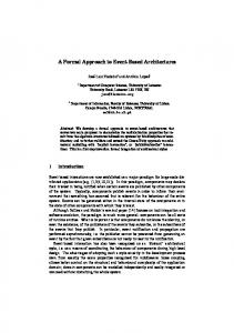
2 THE MATHEMATICAL BASIS OF EVENT CORRELATION 2.1 Causality Graph Models Correlation is concerned with analysis of causal relations among events. We use the notation e→f to denote causality of the event f by the event e. Causality is a partial order relation between events. The relation → may be described by a causality graph whose nodes represent events and whose directed edges represent causality. Figure 2(a) depicts a causality graph on a set of 11 events. To proceed with correlation analysis, it is necessary to identify the nodes in the causality graph corresponding to symptoms and those corresponding to problems. A problem is an event that may require handling while a symptom (alarm) is an event that is observable. Nodes of a causality graph may be marked as problems (P) or symptoms (S) as in Figure 2(b). Note that some events may be neither problems nor symptoms (e.g., event 8) while some other events are both symptoms and problems. The causality graph may include information that does not contribute to correlation analysis. For example, a cycle (such as events 3,4,5) represents causal equivalence. A cycle of events may thus be aggregated into a single event. Similarly, certain symptoms are not directly caused by any problem (e.g., symptoms 7,10) but only by other symptoms. They do not contribute any information about problems that is not already provided by these other symptoms that cause them. These indirect symptoms may be eliminated without loss of information. Henceforth, we will assume that a cauality graph has been appropriately pruned. 2.2 Modeling Causal Likelihood The causality graphs described so far do not include a model of the likelihood (strength) of causality. The causal implication e→f can be considered as a representation of a proposition “e
A Coding Approach To Event Correlation
3
may-cause f." Often, richer information is available describing the likelihood of such causality. Various approaches and measures have been pursued to model such likelihood. A probabilistic model, for example, associates a conditional probability with a causal implication while fuzzy logic associates a fuzzy measure. Each of these models includes operations to compute the strength of a causal chain between two events or to combine the strength of multiple chains between two events. It is useful to have a general model of likelihood that captures these various techniques as special cases. This model must include a set of causal likelihood measures and operations to compute strength of chains and combine them. We proceed to define and demonstrate such a general model of likelihood. Define a semi-ring as a partially ordered set L with an order ≤ and two operations * (catenation) and + (combination) such that: (i) is a semi-group with a unit 1 (a monoid) (ii) is a commutative semi-group with a unit 0 (iii) ∀a,b∈L, a*b≤a,b a,b≤a+b (iv) ∀a∈L, 0≤a≤1 A semi-ring is used to provide a measure of causality. Elements of L provide measures of causal strength with 1 indicating the strongest causality and 0 the weakest. The ordering of likelihood measures is used to compare relative strength of likelihood. The catenation operation is used to compute the strength of causal chains. The combination operation is used to compute the strength of multiple causal chains leading from one event to another. We give a few examples of semi-rings used to model causal likelihood. The deterministic model, uses L=D={0,1} with the order 0≤1. The catenation operation is the Boolean and ∧, with the unit 1, while the combination operation is the Boolean or ∨ with the unit 0. Consider now a causality graph whose edges are all labeled with elements from D. An edge marked 0 represents a highly unlikely causality while an edge marked 1 represents a sure causality. For simplicity assume that all edges marked 0 have been eliminated. The semi-ring structure permits us to assign likelihood to causal chains between two events. The deterministic likelihood of a causal chain such as 1→8→9 in Figure 2 is obtained by catenation (and) and is trivially 1. Now consider the set of causal chains between two events. The likelihood of this set is obtained by applying the combination operation to the likelihood of all causal chains in the set. The deterministic model is a simple and commonly used likelihood model. We now introduce another semi-ring, denoted P, to model probabilistic causality. P consists of the set [0,1] with an ordinary numerical order. The label q on e→f models the conditional probability of the event f when e occurs. The catenation operation is the product of probabilities while the combination operation is defined as q1+q2=1-(1-q1)(1-q2). The temporal model is denoted T. The elements of T are non-negative real numbers representing the expected duration for the respective causality to happen. For example, a label of 8.5 on 1→3 indicates that this causal implication is expected to occur within 8.5 time units (e.g., seconds). The catenation operator * is addition of times (along a causal chain) while the combination operator + is the min operator on real numbers. 0 is the unit with respect to catenation, and ∞ the unit with respect to addition, where ∞ indicates that the causality is unlikely to happen (in any finite time). We use the inverted numerical order as the order on T, modeling
A Coding Approach To Event Correlation
4
“sooner” occurrence of events in time. For example, 6.3≥8.5 should be read as “6.3 happens sooner than 8.5”. Similarly, one can establish fuzzy logic models of causal likelihood or other calculus of uncertainty measures such as the Shafer-Dempster model. Furthermore, by combining various models, more complex likelihood measures may be obtained. For example, the semi-ring defined by PxT ascribes to a causal edge both probability and expected time of occurrence. We are now ready to define a causal likelihood model as a triplet where N is a normal form causality graph, L is a semi-ring describing a likelihood model and φ is a mapping from the edge-set of N to L assigning a likelihood measure to each causal implication. By varying the semi-ring L, a spectrum of models is obtained. 9
1
3
6
11
2
Figure 3: A Correlation Graph 2.3 The Correlation Problem Correlation analysis is concerned with the relationships among problems and the symptoms that they may cause. Consider the correlation relation among problems and symptoms, defined as the closure of the relation → and denoted by ⇒. A correlation p⇒s means that problem p can cause a chain of events leading to the symptom s. This correlation relation may be represented in terms of a bipartite correlation graph. Figure 3 depicts the correlation graph corresponding to the causality graph of Figure 2 after pruning indirect symptoms and aggregating cycles. For a given causal likelihood model one can derive a correlation graph N* corresponding to the causality graph N. Using the catenation operation one can associate a likelihood measure with every causal chain leading from a problem p to a symptom s. The likelihoods of various chains leading from p to s may be combined using the combination operator to provide a likelihood measure of the correlation p⇒s. Thus, for a given causal likelihood model there is a corresponding correlation likelihood model over the correlation graph.
3 THE CODING APPROACH TO EVENT CORRELATION 3.1 Problems, Codes and Correlation The problem of alarm correlation may be now described in terms of the correlation likelihood model. For each problem p, the correlation graph provides a vector of correlation likelihood measures associated with the various symptoms. We denote this likelihood vector as p and call it the code of the problem p. Codes summarize the information available about correlation among symptoms and problems. Code vectors can be best considered as points in an |S|-dimensional
A Coding Approach To Event Correlation
5
space associated with the set of symptoms S, which we call the symptom space. Alarms too may be described as alarm vectors in symptom space assigning likelihood measures 1 and 0 to observed and unobserved symptoms respectively. A very useful reference for coding theory and techniques is provided by [Roman 1992]. The alarm correlation problem is that of finding problems whose codes optimally match an observed alarm vector. We illustrate these considerations using the example of Figure 3. Figure 4(a) depicts a deterministic correlation likelihood model and Figure 4(b) depicts a probabilistic model. Code vectors correspond to the likelihood of the symptoms 3,6,9 in this order. They are given by 1=(1,0,1), 2=(1,1,0) and 11= (1,0,1) for the deterministic model and by 1=(0.8,0,0.3),
3
9
1 1
1
1
1
1
1
0.3
2
11
3
9
6
(a) Deterministic model
1
0.8
0.5
0.9
11
6
0.4
0.9 2
(b) Probabilistic model Figure 4: Correlation Likelihood Models
2=(0.4, 0.9,0) and 11=(0.5,0,0.9) for the probabilistic model. Suppose that alarms consisting of symptoms 3 and 9 have been observed. This may be described by an alarm vector a=(1,0,1). In the deterministic model either 1 or 11 match the observation a and one would infer that the two alarms are correlated with either problem 1 or 11. Note that these two problems have identical codes and are indistinguishable. Similarly, an alarm vector a=(1,1,0) would match the code of problem 2. How should an alarm vector a=(0,1,0) be interpreted? One possibility is that this is just a spurious false alarm. Another possibility is that problem 2 occurred but the symptom 3 was lost. The choice of interpretation depends on whether loss is more likely than spurious generation of alarms. There are, of course, other more remote possibilities. Now, suppose that spurious or lost symptoms are unlikely. The information provided by symptom 9 is redundant. If only symptoms 3 and 6 are observed the respective projections of the codes 1=11=(1,0) and 2=(1,1) are sufficient to distinguish and correlate alarm vectors. Since real alarm correlation problems typically involve significant redundancy. The number of symptoms associated with a single problem may be very large. A much smaller set of symptoms can be selected to accomplish a desired level of distinction among problems. We call such a subset of symptoms a codebook. The complexity of correlation is a function of the number of symptoms in the codebook. An optimal codebook can thus reduce the complexity of correlation substantially. To illustrate this consider an example of 6 problems and 20 symptoms depicted in Figure 5(a). The correlation likelihood model is compactly described in terms of a matrix. Matrix elements represent the correlation likelihood parameters of respective problem-symptom pairs. Figure 5(b) depicts a codebook consisting of 3 symptoms {1,2,4}. This codebook distinguishes among all 6 problems. However, it can only guarantee distinction by a single symptom. For example, problems p2 and p3 are distinguished by symptom 4. A loss or a spurious generation of this symptom will result in potential decoding error. Distinction among problems is measured by the Hamming distance between their codes. The radius of a codebook is one half of A Coding Approach To Event Correlation
6
1 2 3 4 5 6 7 8 9 10 11 12 13 14 15 16 17 18 19 20
p 1 1 1 1 1 1 1 1 1 0 0 0 0 0 0 0 0 0 0 0 0
p 2 0 1 1 0 0 1 0 0 1 1 0 1 1 0 0 1 1 1 1 0
p 3 0 1 0 1 1 1 1 0 0 1 0 0 0 0 1 1 0 1 1 0
p 4 1 1 1 0 1 0 0 1 0 1 1 1 1 0 0 0 1 1 0 0
p p 5 6 0 1 0 0 0 0 1 0 1 0 0 1 0 0 1 1 1 1 0 0 1 0 0 0 1 1 0 1 1 1 0 1 1 0 0 0 1 0 1 1
(a) Correlation Matrix
1 2 4
p 1 1 1 1
p 2 0 1 0
p 3 0 1 1
p 4 1 1 0
p 5 0 0 1
p 6 1 0 0
(b) A Codebook of Radius 0.5
1 3 4 6 9 18
p 1 1 1 1 1 0 0
p 2 0 1 0 1 1 1
p 3 0 0 1 1 0 1
p 4 1 1 0 0 0 1
p 5 0 0 1 0 1 0
p 6 1 0 0 1 1 0
(c) A Codebook of Radius 1.5
Figure 5: A deterministic correlation matrix and codebooks the minimal Hamming distance among codes. When the radius is 0.5, the code provides distinction among problems but is not resilient to noise. To illustrate resiliency to noise consider the codebook of Figure 5(c) where 6 symptoms are used to produce a codebook of radius 1.5. This means that a loss or a spurious generation of any two symptoms can be detected and any singlesymptom error can be corrected. We illustrate the error-correction capabilities of the codebook of Figure 5(c). A minimaldistance decoder will decode as p1 all alarms that contain a single-symptom perturbation of p1. The alarm vectors {011100, 101100, 110100, 111000} will be decoded as a single symptom loss in p1, while {111110, 111101} will be interpreted as occurrence of a spurious symptom. The total number of alarms that can be generated due to a single symptom perturbation (loss or spurious one) in the 6 problems codes + the null problem p0=000000 is 42. Therefore, a total of 48 alarm vectors (out of possible 63) will be correctly decoded despite single-symptom observation errors. When two symptom errors occur a minimal distance decoder can detect that errors have occurred but may not decode the alarm vector uniquely. The considerations above generalize simply to correct observation errors in k symptoms and detect 2k errors as long as k is smaller than the radius of the codebook. Consider now the problem of model errors. That is, what happens when the correlation model itself is incorrect? For example, suppose problem p4 in Figure 5 can actually cause symptom 6 even though the model fails to reflect this. This will cause a single symptom error with respect to the code of p4. Symptom 6 will appear as a spurious symptom whenever p4 occurs. In other words, an error in the correlation model is entirely equivalent to an observation error. In contrast to random observation errors, model errors would appear as persistent observation noise. This persistence may be automatically detected by analyzing correlation logs and then used to correct the correlation model.
A Coding Approach To Event Correlation
7
In summary, one seeks to design minimal codebooks that accomplish a desired level of insensitivity to observation and model errors. This insensitivity to observation errors is measured by the degree to which codes are distinct. In the case of the deterministic model, distinction among codes is measured by the Hamming distance among code vectors. We will soon see that similar measures of distinction may be used to select optimum codebooks in the case of other likelihood models. 3.2 Coding and Decoding The coding technique accomplishes significant correlation speeds. Most of the complexity of correlation computations is handled during the pre-processing of codebook selection. The decoding of alarms in real-time can be very fast. Precise complexity evaluation is beyond the scope of this paper and is left for future publications. However, even crude estimates can usefully illustrate the speed gains. The complexity of decoding is logarithmic in the number of direct decodes (alarm vectors whose errors with respect to codes are less than half the radius of the codebook). The number of direct decodes is bounded by δ(p,c,k)=
( p + 1)
c m m = 0 k
∑
where p is the
number of problems, c is the codebook size (number of symptoms in the codebook) and k is the number of error symptoms to be corrected (Âradius§ - 1). The complexity of decoding is c ]. m m = 0 k
bounded by λ(p,c,k)=lg[ ( p + 1) ∑
For kc). For p=100 the search complexity may be practically infeasible. For example, Nygate and Sterling (1993) report alarm correlation speeds of ECXpert at 0.25 alarms per second for a model involving 10 problems. We proceed to complete the details of codebook design and decoding for a general correlation likelihood model. The point of departure in codebook design is to define a metric of distinction among codes, generalizing the Hamming distance. This is accomplished by using a distance measure on the likelihood semi-ring L. We call a real function d(a,b) on L a distance measure on L if it is symmetric, non-negative and satisfies d(a,a)=0 and d(a,c)≤d(a,b)+d(b,c) for all a≤b≤c in L. Given a distance measure d(a,b) on L, one can extend it to a measure of distinction among code vectors. Define the distance between two code vectors a=(a1,a2,...an) and b=(b1,b2,...bn) as d(a,b)=Σk=1,n d(ak,bk). For example, in the case of the deterministic model define d(1,1)=d(0,0)=0 and d(1,0)=1 to obtain the Hamming distance. For the probabilistic model P, a distance measure is given by the log-likelihood measure d(a,b)=|lg(a/b)| (with lg(0/0)=0 and lg(0/a)=1 for a≠0). For example, in the probabilistic model of Figure 5(b), 1=(0.8,0,0.3) , 11=(0.5,0,0.9) and thus d(1,11)= lg(8/5)+lg(9/3)=lg(24/5). Therefore, in the probabilistic model problems 1 and 11 are distinct, in contrast to the deterministic model. Note that the log-likelihood distance measure generalizes the Hamming distance. When all probabilities are 1 or 0 the two measures yield the same distance.
A Coding Approach To Event Correlation
8
The radius of a set of codes P is defined as the one half of the minimal distance among pairs of codes. The radius provides worst case measure of distinction among code vectors. A codebook C is a subset of the set of symptoms S. The code space defined by C is the respective projection of code vectors in the symptom space defined by S. The radius of the codebook, rC(P) is the respective radius among the projections of codes. Clearly, rC(P)≤ rS(P). Given a desired level of distinction d≤ rS(P), the codebook design problem is that of finding a minimal codebook C for which d≤rC(P). Such codebook provides a guaranteed distinction of at least d among the codes of different problems. The codebook design problem may be solved by a variety of algorithms. A pruning algorithm, for example, can start with the correlation matrix model and eliminate symptoms until an optimal codebook has been established. The algorithm may be designed independently of the specific likelihood model (semi-ring) and distance measure. This may be used to construct a correlator of great generality. Given a codebook C, consider now an alarm vector a describing observed symptoms. The problem of decoding, as discussed above, is to find problem codes that maximally match a. It is useful to utilize a correlation measure µ(a,p) for decoding that is, in general, different from the measure of distinction. We illustrate this through the example of Figure 5(a). Suppose the codebook consists of the symptoms C={3,6}. The codes are 1=11=(1,0) and 2=(1,1). Now consider an alarm vector a=(0,1). The Hamming distances are d(a,1)=d(a,0)=1 and d(a,2)=2, where 0 =(0,0) is the null problem. Thus the Hamming distance does not distinguish between a lost symptom (correlating a with 1) and a spurious symptom (correlating a with 0). In general, a symmetric measure does not distinguish lost from spurious symptoms. We thus permit the correlation measure to be asymmetric. A correlation measure on L consists of two non-negative functions, µ(1,a) and µ(0,a) defined for all a∈L such that µ(1,1)= µ(0,0)=0 and if a≤b, µ(1,a)≥ µ(1,b) while µ(0,a)≤ µ(0,b). For example, in the deterministic case define µ(0,1)=α as the correlation level between an observation of no symptom when the codebook predicts its occurrence, i.e., a lost symptom. Define µ(1,0)=β as the correlation measure between an observation of a symptom that is not included in a code, i.e., a spurious symptom. A correlation measure on L may be easily extended to a correlation measure µ(a,p) between alarm vectors and code vectors. The problem of decoding is to find for a given alarm vector a the problem codes that minimize the correlation measureµ(a,p) -- best match problems. In the probabilistic case let µ(1,a)= |lga| (correlation of occurrence) µ(0,a)=|lg(1-a)| (correlation of non-occurrence). The correlation measure µ(a,p) is given by the logarithm of the product of probabilities assigned by p to events occurring in a and the complements of the probabilities assigned to events that do not occur in a. To illustrate the use of correlation measure in decoding consider again the codebook of Figure 5(c). The correlation measure for the deterministic model is given by µ(0,1)=α (loss) and µ(1,0)=β (spurious). The codebook provides guaranteed error-correction for all single symptom errors. Consider the case when two possible symptom errors occurred. For example, let the alarm vector observed be a=101000. The respective values of the correlation measure for the six problems are 2α, 2α+4β, 2α+β, 2α+β, α+β, 2α+β. Under all choices of α,β the two candidates decodes are p1 (two lost symptoms) and p5 (one lost symptom and one spurious). If α