Tamás Kiss. István Nagy. Adrienn Szabó. Balázs Torma. Data Mining and Web search Research Group, Informatics Laboratory. Computer and Automation ...
Who Rated What: a combination of SVD, correlation and ∗ frequent sequence mining Miklós Kurucz István Nagy
András A. Benczúr Tamás Kiss Adrienn Szabó Balázs Torma
Data Mining and Web search Research Group, Informatics Laboratory Computer and Automation Research Institute of the Hungarian Academy of Sciences
{realace, benczur, kisstom, iscsi, aszabo, torma}@ilab.sztaki.hu ABSTRACT
General Terms
KDD Cup 2007 focuses on predicting aspects of movie rating behavior. We present our prediction method for Task 1 “Who Rated What in 2006” where the task is to predict which users rated which movies in 2006. We use the combination of the following predictors, listed in the order of their efficiency in the prediction:
data mining, recommender systems
• The predicted number of ratings for each movie based on time series prediction, also using movie and DVD release dates and movie series detection by the edit distance of the titles. • The predicted number of ratings by each user by using the fact that ratings were sampled proportional to the margin. • The low rank approximation of the 0–1 matrix of known user–movie pairs with rating. • The movie–movie similarity matrix. • Association rules obtained by frequent sequence mining of user ratings considered as ordered itemsets. By combining the predictions by linear regression we obtained a prediction with root mean squared error 0.256; the first runner up result was 0.263 while a pure all zeroes prediction already gives 0.279, indicating the hardness of the task.
Categories and Subject Descriptors J.4 [Computer Applications]: Social and Behavioral Sciences; G.1.3 [Mathematics of Computing]: Numerical Analysis—Numerical Linear Algebra ∗This work was supported by the Mobile Innovation Center, Hungary, a Yahoo Faculty Research Grant and by grant ASTOR NKFP 2/004/05
Permission to make digital or hard copies of all or part of this work for personal or classroom use is granted without fee provided that copies are not made or distributed for profit or commercial advantage and that copies bear this notice and the full citation on the first page. To copy otherwise, to republish, to post on servers or to redistribute to lists, requires prior specific permission and/or a fee. KDDCup.07, August 12, 2007 , San Jose, California , USA. 2007 Copyright 2007 ACM 978-1-59593-834-3/07/0008 ...$5.00.
Keywords singular value decomposition, item-item similarity, frequent sequence mining
1.
INTRODUCTION
Recommender systems predict the preference of a user on a given item based on known ratings. In order to evaluate methods, in October 2006 Netflix provided movie ratings from anonymous customers on nearly 18 thousand movie titles [5] called the Prize dataset. The KDD Cup 2007 tasks were related to this data set. For Task 1 “Who Rated What in 2006” the task was to predict which users rated which movies in 2006 while for Task 2 “How Many Ratings in 2006” the task was to predict the number of additional ratings of movies. In this paper we present our method for Task 1 “Who Rated What in 2006”. The task was to predict the probability that a user rated a movie in 2006 (with the actual date and rating being irrelevant) for a given list of 100,000 user–movie pairs. The users and movies are drawn from the Prize data set, i.e. the movies appeared (or at least received ratings) before 2006 and the users also gave their first rating before 2006 such that none of the pairs were rated in the training set. We give a detailed description of the sampling method in Section 2.2 since it gives information that we use for the prediction. Our method is summarized as follows: 1. A naive estimate based on a user–movie independence assumption that uses time series analysis and event prediction from the IMDB movie and the videoeta.com DVD release dates as well as the user rating amount reconstructed from sample margins. 2. The implementation of an SVD and an item-item similarity based recommender as well as association rule mining for the KDD Cup Task 1. 3. Method fusion by using the machine learning toolkit Weka [26]. We use the root mean squared error X rmse2 = (wij − w ˆij )2 ij∈R
48
estimated ratings (millions) rmse
4.5 0.262
8 0.255
10 0.256
12 0.257
Table 1: The final rmse as the function of the total estimated ratings R for Task I movies. as the single evaluation measure, where wij is a 0–1 matrix with value 1 if user i gave rating for movie j, and w ˆij is the prediction between 0 and 1 given by the recommender system. The experiments were carried out on a cluster of 64-bit 3GHz P-D processors with 4GB RAM each and a multiprocessor 1.8GHz Opteron system with 20GB RAM. The rest of the paper is organized as follows. In Section 2 we give naive predictions by using the user–movie independence assumption. Then in Section 3 we use three data mining methods: the singular value decomposition, an item-item similarity based recommender and association rule mining to give predictions. The combination of the predictors is described in Section 4. Finally in Section 6 we briefly list related results.
2.
BASE PREDICTION BY USER-MOVIE INDEPENDENCE ASSUMPTION
In this section we give naive estimates that assume independence between the users and the movies. Since for a random variable that has value 1 with probability p and 0 otherwise, the rmse of the prediction of its value is minimized by p, our task is to predict the probability of the existence of a rating, under the independence assumption. As the simplest method, we may predict a constant everywhere. If we correctly guess the number of ratings 7,804 in the 100,000 sample, then this method results in an rmse of 0.268 that would reach 5-6th place in the Cup, indicating the hardness of correctly predicting this value. Notice however that the rmse of 0.279 of the trivial all zeroes prediction would also reach 10-13th place. Next we predict the marginal probabilities and using their product for a “Who Rated What” prediction based on the assumption that movies and users are independent. Notice that this task is highly non-trivial and includes the “How Many Ratings” Task 2 of the KDD Cup as subproblem. We describe our approaches separately for users and movies in the next two subsections. The prediction is given by the product of the marginals scaled so that they sum up to R, the predicted total number of actual ratings for the Task I movies. Given a prediction Nu for the number of ratings of user u, Nm of movie m and denoting the total number of users and movies by U and M , we use Nu · Nm ·R pum = M ·U as the naive prediction for the user–movie pair u, m. We tested how much the prediction depends on correctly estimating R, the total number of ratings. Our prediction for the total number of ratings from the users’ side (Section 2.2) was 4,456,180 while 12,118,700 from the movies’ side (Section 2.1). As shown in Table 1, the result would be slightly better by a lower estimate of 8,000,000 instead of 10,000,000 that we used in our submitted prediction. Notice that our Task II prediction by the same method as we used here only reaches rmse 0.914 compared to the First
Place Winner 0.512 [22]; here rmse is computed over the natural logarithm of the number of ratings plus one. When using their prediction instead of ours we could improve our result by 0.001, a marginal increase in view of the fact that we use a much higher quality input. One reason may be the known property of result mixing to prefer a weaker recommender. Another reason may be that we do not make double use of the information coming from the sampling method as described in Section 2.2. As a final reason, the final error may be dependent on a measure other than the rmse of the logarithm of the number of movie ratings.
2.1 How Many Ratings by Movie The task of predicting the number ratings by the users is basically the same as Task 2 “How Many Ratings in 2006” of the KDD Cup 2007. There the task is to estimate the number of additional ratings for a given movie by users from the Netflix Prize dataset; the only exception is that now another set of movies is used. The set of movies that appeared (or at least received ratings) before 2006 were split randomly into two sets, one per task, resulting in 6822 movies for Task 1 and 8863 for Task 2. Unlike the best performing teams for Task 2 who used the Task 1 movies for training [22], we did not use the fact that the Task 1 user–movie pairs were sampled proportional to the margins (described in detail in Section 2.2). We predict ratings for a given movie by analyzing the time series of its ratings as well as using IMDB movie release and videoeta.com DVD release dates for the movie and its likely series continuation releases. Movie titles across different databases as well as series titles were detected by computing the Damerau-Levenshtein distance [19] between the titles by giving more weight to the prefix of the title and punishing missing complete words less. A stop word removal was also performed first; an extended stop word list included phrases such as “the best of”, “the adventures of” etc. Our prediction is the sum of a base estimated from previous ratings and additional ratings for predicted related release events. We observe an increase in the amount of ratings at and after the dates of related movie and DVD releases, hence if such an event is assumed to happen, then the number of ratings will be estimated higher accordingly. The increase in this case will be proportional to the baseline prediction. The baseline is the total number of ratings of the movie in the period of November 2004 and October 2005. This amount is multiplied by a decay factor, another factor for the DVD release event, and a third factor for series continuation release events for the movie. The factors are trained for year 2005 as the validation period. Movies that appeared in the second half of 2005 were also corrected upwards.
2.2 How Many Ratings by User For predicting the number of ratings of a given user we solely relied on the fact that the sample used for the “Who Rated What” task was taken proportional to the number of ratings of the user. We begin with a detailed description of the sampling method. The 100,000 user–movie pairs were formed by drawing the movies from the 6822 movies selected for Task 1 and the users from the Prize data set, i.e. from those who gave their first rating before 2006. Pairs that corresponded to ratings in the existing Netflix Prize dataset
49
were discarded; we ignored this fact in our prediction. The key difficulty in obtaining the user rating numbers Nu (recall the notations Nu and M as in Section 2) is the small probability of including a single user which implies a high probability of underestimating a single user. In particular we may assume that the actual rating number is non-zero for almost all users that do not appear in the sample. The expected value of the number times the user u is included in the sample equal to 100, 000 · Nu /M . Since Nu /M is very small, the standard deviation of this value is approximately p 100, 000 · Nu /M . While a single user had a very large number of occurrences in the sample, the second largest one occurs only 20 times. For this reason the standard deviation can be assumed to be uniformly below 5. We use this fact by add 4 to the number of appearances in the sample for all users (including those who do not appear at all) and obtain ˆu by scaling to sum up to the estimated total the estimate N number of ratings. To justify the choice of value 4, notice that since the probability of user u not being included in the sample is approximately exp(−100, 000 · Nu /M ), this probability is below 2% for a user with expected number of appearances at least 4.
3.
DATA MINING METHODS
We use three data mining methods, the singular value decomposition, item-item adjusted cosine similarity based recommendation and frequent sequence mining, applied to the known movie rating data. The methods are presented in the above order that also indicates the relative power of their prediction.
3.1
Figure 1: The distribution of the 10-dimensional approximation for user–movie pairs with and without ratings.
SVD based recommendation
For training we use the full 0–1 matrix of all known predictions and use the rank k approximation for prediction. The Singular Value Decomposition (SVD) of a rank ρ matrix W is given by W = U T ΣV with U an m × ρ, Σ a ρ × ρ and V an n × ρ matrix such that U and V are orthogonal. By the Eckart-Young theorem [11] the best rank-k approximation of W with respect to the Frobenius norm is X X (wij − σk uki vkj )2 . ||W − UkT Σk Vk ||2F = ij
where Uk is an m × k and Vk is an n × k matrix containing the first k columns of U and V and the diagonal Σk containing first k entries of Σ. While the Frobenius norm is simply the rmse of the prediction for the existence of the rating, given a uniform sample of user–movie pairs, this is not true for the sampling method used for producing the Task 1 pairs as described in detail in Section 2.2. If the probability that the pair formed by user i and movie j is selected in the sample is pij , then we have to minimize X X pij · (wij − σk uki vkj )2 = ij
ij
our recent experiments [15, 14]. Since we observed overfitting for larger number of dimensions [14] we used the 10dimensional approximation by (1) for prediction where the pij values were obtained as in Section 2. The difference between the distribution of the prediction for actual ratings and no-ratings is seen in Fig. 1.
3.2
k
k
X X√ √ σk uki vkj )2 , ( pij · wij − pij ·
Figure 2: The distribution of the item-item similarity based prediction for user–movie pairs with and without ratings for a similarity top list of size K = 5.
(1)
k
√ which is minimized similarly by the SVD of pij · wij , di√ vided pointwise by pij . In our implementation we used the Lanczos code of svdpack [6] that turned out both fastest and most precise in
Item-item similarity based recommendation
We computed the adjusted cosine similarity [23] for an item-item based recommender that recommends an unrated movie j to a given user i by the weighted average of the nearest K movies to i rated by the user. Here K is a parameter; roughly speaking, this approach increases the fraction of known values by a factor of K. By observing the difference of the prediction for user–movie pairs with and without ratings in Fig. 2 we use K = 5.
3.3
Association Rules in Sequences
We used an APRIORI [2] implementation for frequent sequence mining. We discarded all movies that received more than 50,000 ratings and all users that gave more than 3,000 ratings in the Prize data set. We added the condition that in a frequent sequence the number movie ratings must not differ by more than a factor of 4; since this property is monotonic, we could implement a filter in the APRIORI algorithm. We restricted sequences for time windows of 30 days; we allowed all permutations of movies that received their
50
the sample.
4.1
Performance of subset combinations
We measured the effect of some interesting combinations as well, all of which are still first place winner. By using the naive prediction (Section 2) we obtain rmse 0.260 with 0.6374 · pum + 0.025. If we only add SVD, 0.5533 · pum + 0.1987 · SVD + 0.0016 gives rmse 0.256 and without SVD we have 0.59 · pum
+
0.0962 · correlation + 0.1 · assoc rules − Figure 3: Rating number shows the fraction of the 100,000 pairs of the task where we give rating x. Hit ratio shows the fraction of actual ratings with predicted value x. The horizontal axis shows x, binned into intervals of 0.01. ratings from the user on the same day. We set the minimum support to 50. Given the frequencies of the sequences with the above constraints, stored in a trie, we proceed by giving prediction to a user–movie pair as follows. We select all frequent sequences that terminate with the given movie m and select the longest subsequence m1 , . . . , ms rated by the user. Next we compute the confidence of the association rule m1 , . . . , ms ← m by looking up the frequencies of sequences m1 , . . . , ms and m1 , . . . , ms , m, both of which are frequent by definition. Finally we use the maximum of the confidence of all rules that fit the user–movie pair as prediction.
4.
COMBINATION OF METHODS
We combined the four predictions of the naive independence, SVD, item-item correlation and association rule based approaches by the linear regression method of the machine learning toolkit Weka [26]. We obtained the equation 0.5533 · pum 0.029 · correlation 0.1987 · SVD −0.0121 · assoc rules
+ + + −
with rmse 0.261, justifying the power of all three methods with the superiority of SVD. The result without using the probabilities estimated from the sample would be 0.2673, achieving place 4–5 in the KDD Cup with 0.0758 · correlation + 0.2787 · SVD + 0.0669 · assoc rules + 0.0049.
4.2
as the final prediction that reaches rmse 0.256, gaining 0.007 over the first runner up and 0.023 over a pure all zeroes prediction. Surprisingly the correlation based recommender has very small while the association rules have negative coefficient. This indicates that most of their information is already included in the SVD. In fact the predictive power of frequent sequences is likely already over-represented by the SVD and the correlation based recommender. We show how well the predicted probability of an actual rating given in 2006 fits to the real data. In Fig. 3 we depict the fraction of actual ratings within the 100,000 user–movie pairs of Task I and the fraction of those with prediction x, both as a function of x. The picture becomes unstable over x = 0.5 due to the small number of very high predicted values. In the useful range the fraction of actual ratings increase with the prediction x very close to linear, as required by an optimal solution. The point where the curves meet is also very close to the 0.078 fraction of actual ratings within
An alternate method of combination
In a preliminary version we used an alternate, seemingly less sophisticated method to combine predictions. This method to be sketched below however performed only marginally worse, still reaching first place in the competition and may be of possible further use for combining predictions. As seen in Figs. 1 and Fig. 2, for a given predicted value x we can count (in the training set of Year 2005 data) the fraction of actual ratings with the predicted value x. By using a binning of step 0.1 we made 10 prediction values, one for each range, given by the above fraction. For ranges where the data was sparse (see x > 0.5 in Fig. 3 as illustration) we used manual correction. Finally we took the maximum as the final prediction.
5. 0.0042
0.0027,
CONCLUSION AND DISCUSSION
The main lesson learned is probably the fact that very different data mining techniques catch very similar patterns in the data that makes it increasingly difficult to improve prediction quality beyond certain point. We also demonstrated the hardness of the task by showing how well trivial estimates perform, just marginally outperformed by our result and beating most of the contestant teams. Just as it is the case for Task II, the information leaked by the sampling method used to generate the test user–movie pairs could be used. While without reconstructing marginals it would likely have been impossible to come within first three, data mining methods however did well without this help as well. In the current task low rank approximation performed best, a phenomenon more or less considered “fact” by the movie ratings recommender community. Note that a relative carefully tuned item-item recommender performed very close the association rules. We stress here that tuning association rule based prediction is a very time (and CPU) consuming task and our method is far from being the result of an exhaustive experimentation. In particular pruning thresholds were chosen by ad hoc investigation of a small number of runs. Also we did not incur lower limits on confidence that might have improved performance.
51
6.
RELATED WORK
Recommenders based on the rank k approximation of the rating matrix based on the first k singular vectors are probably first described in [7, 21, 12, 24] as well as several papers of that era. Several authors give theoretical analysis for the performance of SVD in a recommender system [10, 4, 9]. Unlike in the “Who Rated What” question, a recommender system typically has to handle the fact that users only rate part of the items that are of their potential interest; for this task an expectation maximization based SVD algorithm can be given [8, 25, 28, 14]. Item-item correlation based recommenders appear first in [23] who describe correlation, cosine and adjusted cosine similarity as possible bases for a recommender. The adjusted cosine similarity, a slight modification of the Pearson correlation where the ratings of the nearest movies are corrected by their movie averages performs best both in [23] and our experiments. The method is also used by Amazon.com [16] who note that the algorithm scales very well with the number of users. Frequent itemset mining was introduced by [1]; the APRIORI algorithm is first described in [2] that can easily be modified to mine frequent sequences [3]. Although more efficient algorithms were introduced since then for the frequent itemset [27, 13] and frequent sequence [20] mining tasks, we chose APRIORI as the base of our algorithm due to its simplicity and ease of implementation and modification. Using association rules and sequential patterns for prediction has been studied for a while, e.g., by Liu et al. [18], see also the related section in [17].
7.
[8]
[9]
[10]
[11] [12]
[13]
[14]
REFERENCES
[1] R. Agrawal, T. Imielienski, and A. Swami. Mining association rules between sets of items in large databases. In P. Bunemann and S. Jajodia, editors, Proceedings of the 1993 ACM SIGMOD Conference on Managment of Data, pages 207–216, New York, 1993. ACM Press. [2] R. Agrawal and R. Srikant. Fast algorithms for mining association rules. In J. B. Bocca, M. Jarke, and C. Zaniolo, editors, International Conference on Very Large Data Bases (VLDB), pages 487–499. Morgan Kaufmann, 12–15 1994. [3] R. Agrawal and R. Srikant. Mining sequential patterns. In P. S. Yu and A. L. P. Chen, editors, Processing of the 11th International Conference on Data Engineering (ICDE’95), pages 3–14. IEEE Press, 6–10 1995. [4] Y. Azar, A. Fiat, A. R. Karlin, F. McSherry, and J. Saia. Spectral analysis of data. In Proceedings of the 33rd ACM Symposium on Theory of Computing (STOC), pages 619–626, 2001. [5] J. Bennett and S. Lanning. The netflix prize. In KDD Cup and Workshop in conjunction with KDD 2007, 2007. [6] M. W. Berry. SVDPACK: A Fortran-77 software library for the sparse singular value decomposition. Technical report, University of Tennessee, Knoxville, TN, USA, 1992. [7] D. Billsus and M. J. Pazzani. Learning collaborative information filters. In ICML ’98: Proceedings of the Fifteenth International Conference on Machine
[15]
[16]
[17] [18]
[19] [20]
[21]
[22]
[23]
Learning, pages 46–54, San Francisco, CA, USA, 1998. Morgan Kaufmann Publishers Inc. J. Canny. Collaborative filtering with privacy via factor analysis. In SIGIR ’02: Proceedings of the 25th annual international ACM SIGIR conference on Research and development in information retrieval, pages 238–245, New York, NY, USA, 2002. ACM Press. P. Drineas, I. Kerenidis, and P. Raghavan. Competitive recommendation systems. In Proceedings of the 34th ACM Symposium on Theory of Computing (STOC), pages 82–90, 2002. K. Goldberg, T. Roeder, D. Gupta, and C. Perkins. Eigentaste: A constant time collaborative filtering algorithm. Inf. Retr., 4(2):133–151, 2001. G. H. Golub and C. F. V. Loan. Matrix Computations. Johns Hopkins University Press, Baltimore, 1983. D. Gupta, M. Digiovanni, H. Narita, and K. Goldberg. Jester 2.0 (poster abstract): evaluation of an new linear time collaborative filtering algorithm. In SIGIR ’99: Proceedings of the 22nd annual international ACM SIGIR conference on Research and development in information retrieval, pages 291–292, New York, NY, USA, 1999. ACM Press. J. Han, J. Pei, and Y. Yin. Mining frequent patterns without candidate generation. In W. Chen, J. F. Naughton, and P. A. Bernstein, editors, Proceedings of the 2000 ACM SIGMOD International Conference on Management of Data, pages 1–12. ACM Press, 2000. M. Kurucz, A. A. Bencz´ ur, and K. Csalog´ any. Methods for large scale svd with missing values. In KDD Cup and Workshop in conjunction with KDD 2007, 2007. M. Kurucz, A. A. Bencz´ ur, K. Csalog´ any, and L. Luk´ acs. Spectral clustering in telephone call graphs. In WebKDD/SNAKDD Workshop 2007 in conjunction with KDD 2007, 2007. G. Linden, B. Smith, and J. York. Amazon.com recommendations: item-to-item collaborative filtering. Internet Computing, IEEE, 7(1):76–80, 2003. B. Liu. Web Data Mining: Exploring Hyperlinks, Contents and Usage Data. Springer, 2006. B. Liu, W. Hsu, and Y. Ma. Integrating classification and association rule mining. In ACM International Conference on Knowledge Discovery and Data Mining (SIGKDD), 1998. G. Navarro. A guided tour to approximate string matching. ACM Comput. Surv., 33(1):31–88, 2001. J. Pei, J. Han, B. Mortazavi-Asl, H. Pinto, Q. Chen, U. Dayal, and M.-C. Hsu. PrefixSpan mining sequential patterns efficiently by prefix projected pattern growth. In Proc. 2001 Int. Conf. Data Engineering (ICDE’01), pages 215–226, 2001. M. H. Pryor. The effects of singular value decomposition on collaborative filtering. Technical report, Dartmouth College, Hanover, NH, USA, 1998. S. Rosset, C. Perlich, and Y. Liu. Making the most of your data: Kdd cup 2007 how many ratings winners report, 2007. B. Sarwar, G. Karypis, J. Konstan, and J. Reidl. Item-based collaborative filtering recommendation
52
[24]
[25]
[26]
[27]
[28]
algorithms. In WWW ’01: Proceedings of the 10th international conference on World Wide Web, pages 285–295, New York, NY, USA, 2001. ACM Press. B. Sarwar, G. Karypis, J. Konstan, and J. Riedl. Application of dimensionality reduction in recommender systems–a case study. In ACM WebKDD Workshop, 2000. N. Srebro and T. Jaakkola. Weighted low-rank approximations. In T. Fawcett and N. Mishra, editors, ICML, pages 720–727. AAAI Press, 2003. I. H. Witten and E. Frank. Data Mining: Practical Machine Learning Tools and Techniques. Morgan Kaufmann Series in Data Management Systems. Morgan Kaufmann, second edition, June 2005. M. J. Zaki, S. Parthasarathy, M. Ogihara, and W. Li. New algorithms for fast discovery of association rules. In D. Heckerman, H. Mannila, D. Pregibon, R. Uthurusamy, and M. Park, editors, In 3rd Intl. Conf. on Knowledge Discovery and Data Mining, pages 283–296. AAAI Press, 12–15 1997. S. Zhang, W. Wang, J. Ford, F. Makedon, and J. Pearlman. Using singular value decomposition approximation for collaborative filtering. In CEC ’05: Proceedings of the Seventh IEEE International Conference on E-Commerce Technology (CEC’05), pages 257–264, Washington, DC, USA, 2005. IEEE Computer Society.
53