A Comparative Study of Implicit and Explicit Methods Using Unstructured Voronoi Meshes in …
Francisco Marcondes
Member, ABCM
[email protected] Federal University of Ceará – UFC Dep. of Metallurgical Eng. and Material Sci. 60341-790 Fortaleza, CE, Brazil
Clovis R. Maliska
[email protected] Federal University of Santa Catarina – UFSC Department of Mechanical Engineering 88040-900 Florianópolis, SC, Brazil
Mário C. Zambaldi
[email protected] Federal University of Santa Catarina – UFSC Department of Mathematics 88040-900 Florianópolis, SC, Brazil
A Comparative Study of Implicit and Explicit Methods Using Unstructured Voronoi Meshes in Petroleum Reservoir Simulation This work presents a comparative study among three linearization schemes widely used in petroleum reservoir simulation, namely the Implicit Pressure Explicit Saturation (IMPES), Fully Implicit (FI) and Adaptive Implicit Method (AIM). Attention is given to the criterion used for switching from IMPES to FI and vice-versa. The black-oil model considering the oil-water flow is employed. The equations are discretized using an unstructured Voronoi mesh in a finite-volume framework. The numerical results are analyzed based on the number of iterations in the Newton and solver procedures, number of implicit volumes, and mass balance error of components. The effect of the stopping criterion on Newton's iterations is also investigated. The outcome of the study reveals that adaptive implicit methodologies can be a good choice when unstructured grids are present, allowing the use of time steps with the same order of magnitude as the ones used in FI procedures, but with reduction in the computational effort. Keywords: adaptive implicit method, voronoi grids, finite-volume method, petroleum reservoir simulation
Introduction 1 IMPES is one of the most widely used procedures in petroleum reservoir simulation. In this scheme the mobilities are evaluated with saturation and pressure from the previous time level. This fact decouples the pressure equation from the saturation equations, allowing the saturation to be calculated explicitly, while pressure is kept implicit. Such a scheme requires a small computational effort per timestep, because the pressure is the only unknown to be calculated through a linear system of equations. Another advantage is that the procedure for advancing the saturation is easily vectorized. The main disadvantage of IMPES is that the CourantFriedrichs-Lewy (CFL) number must be smaller than unity, to avoid spurious oscillations in the solution. On the other hand, a methodology which works well with CFL larger than unity is the Fully Implicit (FI) one, which solves pressure and saturation simultaneously. However, the computational effort per timestep increases considerably when compared with IMPES. According to Thomas and Thurnau (1983), except in some critical regions of the reservoir, such as in the vicinity of the wells or near saturation fronts, the IMPES method can work with reasonable large time steps. From this observation, Thomas and Thurnau (1983) proposed the use of the Adaptive Implicit Method (AIM), whose concept was later improved by Forsyth Jr. and Sammon (1986). The goal of the Adaptive Implicit Method is to advance saturation and pressure implicitly in the regions where the CFL is larger than unity or where large variations in the saturations occur. In other regions of the reservoir only the pressure is considered implicitly. One of the difficulties of the AIM implementation is the switching criterion to change the procedure to FI and vice-versa. Thomas and Thurnau (1983) used as switching criterion a specified saturation threshold from the previous iteration level. If an IMPES volume experiences a variation in saturation larger than the specified threshold, this volume is calculated as being FI in the next Newton's iteration. Forsyth Jr. and Sammon (1986) found that this criterion does not allow a new cell to become IMPES again once it was switched to FI, because a FI cell can have large throughput and the variation in saturation can be small. In this case, if this volume is switched to IMPES large instabilities may result. Russel (1989)
Paper accepted July, 2009. Technical Editor: Celso K. Morooka
J. of the Braz. Soc. of Mech. Sci. & Eng.
proposed a criterion based on the CFL number to determine which volume may switch from FI to IMPES and vice-versa. He provides several reasons for working with the criterion based on the CFL and several ways to approximately calculate it. Nevertheless, it does not present any result for two and three phase flows. Young and Russel (1993) proposed a new relation for calculating the CFL number and suggest applying it in conjunction with the calculation of the maximum variation in the saturation. In this case, solutions using the IMPES method with the CFL larger than unity were obtained without oscillations. Fung et al. (1989) proposed a criterion based on the local analysis of the approximate equations. In each volume the eigenvalues are calculated and recommended that the spectral radius be smaller than unity for treating the cell with the IMPES method. Otherwise, the volume must be considered by the FI procedure. This scheme was applied to three-phase flow in Cartesian grids only. The objective of this work is to present a comparison among the above discussed methodologies employing unstructured Voronoi meshes, broading the range of application of adaptive implicit methods. The results are presented in terms of CPU time, number of Newton’s iterations, number of time iterations, and the degree of implicitness. The stability criterion proposed by Fung et al. (1989) added to a specified variation in the saturation field was adapted to deal with arbitrary number of connections between control volumes. The black-oil model is employed and two-phase (oil-water) in twodimensional case studies are investigated.
Nomenclature A
= reservoir area, m2
AIM = Adaptive Implicit Method bij = width of the face located between the gridpoints i and j, m c = compressibity of the fluid, Pa-1 B = volumetric formation factor dij = distance between the grid points i and j, m MBE = mass balance error FI = Fully Implicit method h = height of the reservoir, m IMPES = Implicit Pressure Explicit Saturation method J = Jacobian matrix K = absolute permeability, m2 kr = relative permeability
Copyright © 2009 by ABCM
October-December 2009, Vol. XXXI, No. 4 / 353
Francisco Marcondes et al.
M Nν NIN NIT P Pc PI Pi PVI
= viscosity ratio = number of neighbors of control volume i = total Newtonian iterations = number of time steps = pressure, Pa = capillarity pressure, Pa = percentage of implicit control volumes = initial pressure, Pa = porous volume injected q = volumetric flow rate at storage conditions per unit of reservoir volume, (m3/s)/m3 qpi = injected volumetric flow rate, m3/s qpp = produced volumetric flow rate, m3/s r = vector of residues rrw = well radius, m R = residue of Newton's equation R* = R multiplied by the inverse of the diagonal matrix block Sor = residual oil saturation S = saturation t = time, s T = transformation matrix TCPU = total CPU time Tij = transmissibility factor = Volume of the control volume, m3 Vi Vf,p = final volume of phase p, m3 Vi,p = initial volume of phase p, m3 x',y' = local coordinate system X = represent P or Sw Greek Symbols * ∆Pmax = maximum pressure variation, Pa * ∆S max = maximum saturation variation ∆S w = threshold change in the water saturation ∆X = increment or decrement in X ∆t = timestep, s
α φ λ λ1 λ2 µ ε εn εn+1 ρ
where φ is the porosity and Bp is the volumetric formation factor, P is the pressure in the reservoir, q p is the volumetric flow rate at stock tank conditions per unit volume of the reservoir. The mobility, λp, is defined as
λp = K
krp
where K is the absolute permeability, krp is the relative permeability and µp is the viscosity of phase p. In Equation (2), the volumetric formation factor is included in the mobility phase because the volumetric balance is evaluated at stock tank conditions. Writing Eq. (1) for the oil and water phases there are three unknowns (So, Sw and P) and only two equations. The closure equation comes from the global mass conservation, given by
S w + So = 1
(3)
The velocity field can be found from the Darcy's equation. Details can be found in Aziz and Setari (1979).
Integration of the Governing Equations Figure 1 shows a control volume of Voronoi type, where i indicates the gridpoint and the j's are its neighbors. For each gridpoint j, it is possible to align a local Cartesian system x'-y' in so that the x' axis (the line that joins gridpoints i and j) be perpendicular to the face of the control volume, allowing the evaluation of the fluxes using only two gridpoints, a property of local orthogonal grid systems (Palagi and Aziz, 1994).
= eigenvalues = porosity = mobility = bound for forward switching = bound for backward switching = viscosity, Pa.s = user tolerance = error in the time level n = error in the time level n+1 = spectral radius Figure 1. Control volume of Voronoi type.
Subscripts w o p
(2)
µ p Bp
denotes water phase or well denotes oil phase denotes phase p
Integrating Eq. (1) in space and in time, one obtains: n +1
Mathematical Model Assuming there are only two immiscible phases in the reservoir, oil (o) and water (w), and neglecting the gravitational and the capillarity pressure effects, the volumetric conservation equation for the phase p can be written as
∂ ⎛ Sp ⎞ ⎜φ ⎟ = ∇. ⎡⎣λ p .∇P ⎤⎦ + q p ∂t ⎜⎝ B p ⎟⎠
354 / Vol. XXXI, No. 4, October-December 2009
(1)
⎛ φV S p ⎞ ⎜ ⎟ ⎜ ∆t B p ⎟ ⎝ ⎠i
n
Nν ⎛ φV S p ⎞ −⎜ ⎟ = ∑ Tij λijn +θ ( Pjn +1 − Pi n +1 ) + q np+θ ⎜ ∆t B p ⎟ ⎝ ⎠i j =1
(4)
The superscript θ in Eq. (4) identifies the type of the procedure: θ = 1, FI; θ = 0, IMPES; and if θ assumes zero or one in different regions of the domain, the procedure is AIM. Nν is the number of neighbors of control volume i, and Tij is the transmissibility, given by
⎛ bhK ⎞ Tij = ⎜ ⎟ ⎝ d ⎠ij
(5)
ABCM
A Comparative Study of Implicit and Explicit Methods Using Unstructured Voronoi Meshes in …
where b and d are shown in Fig. 1 and h is the thickness of the control volume.
FI, IMPES and AIM Formulations FI Formulation In this formulation, the unknowns pressure P and the water saturation Sw are obtained simultaneously. For the mobilities, ⎛ krp ⎜ ⎜ µ p Bp ⎝
⎞ ⎟ , krp,ij is computed using UDS (upstream differencing ⎟ ⎠ij
scheme) and (µpBp)ij using an arithmetic averaging of the corresponding values at the gridpoints ij. The system of equations is solved iteratively using Newton's method. Making θ = 1 in Eq. (4), for all control volumes, the residual form of the equation reads
n
ν
∆X ν +1 = − R*ν
After solving Eq. (11) for ∆X ν +1 , P is obtained by
Pν +1 = Pν + ∆X ν +1
(6)
where Jij are the coefficients of the second line of control volume i, according to Fig. 2c.
(a)
P
Sw
X 0
...
X 0
ν
(7)
where ν is the iteration level and X represents the unknowns (P and Sw). When convergence is achieved the residue in the iteration ν+1 should be zero. Therefore, ν
P (b)
(c)
Sw
X X X X P
Sw
X 0 P
P
X
1
X 0
...
...
− Pressure equation
P
...
Sw
1 0 0 1
X
(8)
The unknowns (P and Sw) are calculated after each Newtonian iteration, as
X ν +1 = X ν + ∆X ν
(13)
j =1, j ≠ i
P
⎛ ∂Rip ⎞ ν +1 ν ∑⎜ ⎟ ∆X = − Rip ; p = o, w ∀X X ∂ ⎝ ⎠
(12)
and Sw by
The Taylor series expansion of the residue gives
⎛ ∂Rip ⎞ Rνip +1 = Rνip + ∑ ⎜ ⎟ ∆X ∀X ⎝ ∂X ⎠
(11)
S wn,+i 1 = ∑ ∆X ν +1 J i , j + Rw*ν,i
Nν
⎛ φV S p ⎞ +⎜ ⎟ ; p = o, w ⎜ ∆t B p ⎟ ⎝ ⎠i
[J ]
Nν
n +1
⎛ φV S p ⎞ Rip = ∑ Tij λijn +1 ( Pjn +1 − Pi n +1 ) + q np +1 − ⎜ ⎟ ⎜ ∆t B p ⎟ j =1 ⎝ ⎠i
shown in Fig. 2a. To obtain the pressure equation, each Jacobian block line is multiplied by its inverse diagonal block resulting in the block line of Fig. 2b. Also, the inverse of each diagonal block is ν *ν multiplied by the original vector Ri , resulting in the Ri vector. As shown in Fig. 2c, the pressure equation is decoupled from the saturation equation. When this procedure is applied to each control volume, the pressure equation is obtained using the first line of each block of Fig. 2c, yielding the system
X 0 X 0 P
...
Sw
Sw
X 0 X 0 P
... 1
X X
− Saturation equation
Figure 2. Steps for obtaining the pressure equation for the IMPES method.
(9) AIM Formulation
and the procedure is stopped when the following tolerances are satisfied: ν +1 * +1 ∆Pmax ≤ ∆Pmax ; ∆Sνw,max ≤ ∆S w* ,max
(10)
* where ∆Pmax and ∆S w* ,max are input parameters.
IMPES Formulation In this procedure, the terms which contain the fluid, mobility and the production or injection flow rates are based on the saturation and pressure from the previous time level. Making θ = 0 in Eq. (4), a similar equation to Eq. (6) is obtained. All terms depending on the saturation are explicitly calculated, except the term which involves the saturation at the level (n+1)-th, which is, in fact, the required transient term. Therefore, when Newton's linearization is applied in each Jacobian block line, the only full block is the diagonal one, as J. of the Braz. Soc. of Mech. Sci. & Eng.
The IMPES scheme requires considerably less computational effort per timestep than the FI. However, it is often limited to small timesteps due to instabilities inherent to explicit schemes. This occurs in regions where the velocities or gradients of saturation are high. On the other hand, in the FI scheme the size of the timestep is bounded only by the accuracy of the solution. The goal of the AIM method is to put together the advantages of each methodology, using the FI method in the regions where the IMPES method shows instabilities and IMPES in the rest of the reservoir. Recall that pressure is evaluated implicitly all over the reservoir. Evaluating the production/injection terms implicitly and considering that the mobilities of the phases can be considered implicit (FI) or explicit (IMPES), a similar equation to Eq. (6) is obtained. Using the same procedure used for the pressure equation in the IMPES method, a similar equation to Eq. (11) is obtained, where the only difference is that the entries of the Jacobian matrix can be blocks (1x2), (2x1), (2x2) or (1x1).
Copyright © 2009 by ABCM
October-December 2009, Vol. XXXI, No. 4 / 355
Francisco Marcondes et al.
Switching from an IMPES to a FI Volume and Vice-versa The success of an AIM scheme depends strongly on the efficiency of the switching criterion. A sensitive and practical criterion is not easily found. Here a local stability criterion of the Jacobian matrix akin to the one proposed by Fung et al. (1989) is employed. Denoting the residue of the conservation equations by R and the variables (P and Sw) by X, Newton's iteration can be written, in the index notation, as
X
n +1,ν +1 i
=X
n +1,ν i
⎛ ∂R n +1,ν − ⎜ in +1,ν ⎜ ∂X j ⎝
−1
⎞ ⎟ Rin +1,ν ; i, j = 1,..., N ⎟ ⎠
(14)
where N is the total number of equations. In Eq. (14), X in +1,ν +1 is n +1,ν is the residual at the solution in the (ν+1)-th iteration, and R j n +1 converges when the ν-th iteration of the i-th equation. X i
X in +1,ν +1 − X in +1,ν
∞
≤ ε . The term dRin +1,ν +1 is written as
⎛ ∂R n +1,ν +1 ⎞ ⎛ ∂R n +1,ν +1 ⎞ dRin +1,ν +1 = ⎜ i n, m ⎟ dX nj , m + ⎜ in +1,ν +1 ⎟ dX nj +1,ν +1 ≈ 0 ⎜ ∂X j ⎟ ⎜ ∂X j ⎟ ⎝ ⎠ ⎝ ⎠
(15)
where m refers to the last iteration at the time level n. If the error at n and ε n +1 , the time levels n and n+1 are denoted by ε respectively, Eq. (15) can be written as
⎛ ∂Rin +1,ν +1 ⎞ n +1 ⎛ ∂Rin +1,ν +1 ⎞ n ⎜ ⎟ε = ⎜ ⎟ε ; ⎜ ∂X nj +1,ν +1 ⎟ j ⎜ ∂X nj , m ⎟ j ⎝ ⎠ ⎝ ⎠
i, j = 1,..., N
(16)
where the signal of ε is neglected, since only its norm is of interest. Considering
⎛ ∂R n +1,ν +1 ⎞ T = ⎜ in +1,ν +1 ⎟ ⎜ ∂X j ⎟ ⎝ ⎠
−1
⎛ ∂Rin +1,ν +1 ⎞ n ⎜ ⎟ε ⎜ ∂X nj , m ⎟ j ⎝ ⎠
(17)
important simplifications are convenient and produce good results. The accumulation term at time level n can be excluded from Ri. For the evaluation of the derivatives, the flow is considered incompressible, which simplifies the calculation of the eigenvalues. Tests without this assumption produced similar results. In the original proposal of Fung et al. (1989), three eigenvalues are required for all control volumes. To avoid that, they suggested that only the eigenvalues at the boundary between implicit and explicit regions be calculated. This implies that when there is a switching in the tested control volume, all the explicit neighbors must be checked, if the switching is from explicit to implicit (forward switching). Otherwise, if the switching is from implicit to explicit (backward switching), all the implicit neighbors must be checked. This procedure should be repeated until no volumes should be switched. Recalling that the compressibility effects are small in oil-water flows, the incompressibility condition was considered for calculating the eigenvalues. This implies that only one eigenvalue need to be calculated for each control volume, allowing, due to the minor computational effort required, the calculation of the eigenvalues for all control volumes. It was not possible to reproduce the implicit front reported by Fung et al. (1989) using these stability criteria. However, considering the compressibility effects and calculating the two eigenvalues for all control volumes, the results were identical. A possible reason for that is because one is solving two-phase flows, while in the work of Fung et al. (1989) three-phase flows were treated. Searching for a more robust switching criterion, the following results where obtained with the method just described in conjunction with a switching criterion based on the variation of the saturation. The errors in the mass balance of oil and water are also reported on the tables of results. The mass balance error of each component, MBEp, is calculated by
(
)
MBE p = Vi , p + ∑ qwi ∆t − ∑ ql ∆t − V f , p / ∑ qwi ∆t
(21)
where Vi,p and Vf,p are the initial and final volumes of phase p in a specified time level, qwi is the volumetric flow rate of injected water and ql is the volumetric flow rate of the producing liquid (oil+water). The numerator of Eq. (21) represents the error in the volume of the phase p, in each time level, and the denominator the volume of injected water, both integrated from the starting.
Eq. (16) can be written as
ε nj +1 = T ε nj
(18)
All cases analyzed in this section were obtained with
where T is the transformation matrix. The condition of stability is
ε in +1 ≤ ε in
(19)
which guarantees that the error introduced in a specified time level is not amplified in the next one. This condition is satisfied if T is normal and
ρ (T ) = max ≤ α j (T ) ≤ 1 i≤ j≤ N
(20)
where αj’s are the eigenvalues of T, and ρ(T) is the spectral radius of T. These are the stability conditions of the whole system. Computing the spectral radius is obviously impracticable. One can however identify the control volumes that yield instability by computing easily the spectral radius of its respective small submatrix. Eq. (18) can be written for each control volume and the maximum eigenvalue of T calculated. If the Eq. (20) holds, the cell can be IMPES, otherwise it is FI (see Fung et al. 1989). Two 356 / Vol. XXXI, No. 4, October-December 2009
Results * ∆Pmax = 68,95 kPa and ∆S w* ,max = 5 x10⁻³ . Similar CPU time were
observed between the AIM and FI methodology for tests with * ∆S w* ,max = 10−3 and ∆Pmax = 68,95 kPa. For the AIM and FI methodologies, Newton's iteration is performed until the variation in saturation and pressure satisfies the tolerance for every control volume, regardless whether the saturation was treated explicitly or implicitly. As expected, the number of Newton's iterations increased considerably per timestep in the IMPES method. For the sake of comparison among the methodologies, all of them used the Jacobian matrix structure. Therefore, no criterion based on pre-fixed values was used for the IMPES method. For all cases the GMRES solver (Saad and Schultz, 1986) with ILU(1) preconditioning was employed. In all tables of results, the eigenvalues λ1 is the bound for the forward switching, λ2 is the bound for the backward switching, and ∆Sw is the threshold change in the water saturation used for the implicit switching. They are listed as (λ1, λ2, ∆Sw), and the missing value, denoted by (*) means that the respective criterion was not used. ABCM
A Comparative Study of Implicit and Explicit Methods Using Unstructured Voronoi Meshes in …
Using the threshold change in the saturation, whenever a cell is switched, all its neighbors are checked out. For the backward switching, some tests were done to find out how frequent it must be checked. The switching after 20 iterations in time provides good results. Switching after 10, 20, 30 and 50 iterations is also considered. For all cases the results are reported for a dimensionless time level (PVI) equal to 1.82, that is, the volume of liquid injected is 1.82 times the porous volume of the reservoir. Also NIN is the total Newtonian iterations, NIT and PI are, respectively, the number of timesteps and the percentage of implicit control volumes required to reach 1.82 PVI. The CPU time were normalized by the minimum CPU time among the methods. For evaluating the pressure and saturation, an integration process with a variable timestep is used as in Aziz and Settari (1979). Except for the IMPES method, the timestep used was up to 50 days. The first test case, CASE 1, considers a flow whose relative permeability curves are quadratic functions of the saturation. The hybrid grid is shown in Fig. 3, the physical and geometric data are listed in Tab. 1, and the relative permeability and viscosity ratio curves are given by
krw =
S w2 µ ; kro = 1 − kw ; M = o µw M (1 − S w2 ) + S w2
approach. In this case, there is a large difference in the number of Newtonian iterations, meaning that the criterion used by the AIM method does not detect the regions of appearance of instabilities. Also, the errors of the IMPES mass balance are larger than the AIM and FI. This fact can be explained considering that only one Newtonian iteration is performed, and the same convergence criterion in the solver for the three schemes was employed. For M = 10, Figure 4 presents the implicit fronts for four PVI values. In this case λ1 = 1.0, λ2 = 0.8, and ∆Sw = 0.01. It is verified that for higher PVI values only a small number of volumes were kept implicit. There is a considerable reduction in the number of implicit cells from 0.2 to 0.6 PVI. This occurred because the water front at 0.6 PVI had already reached the producing wells. After the water breakthrough, the number of implicit cells decreases proportionally to the increasing of the saturation in the wells. The water breakthrough occurs at 0.3 PVI approximately, according to Fig. 6.
(22)
FI
IMPES
Figure 3. Five-spot problem. Hybrid-hexagonal grid with 445 volumes.
Table 1. Physical and geometrical data of the reservoir – case 1.
Reservoir data K = 12.5 x 10⁻¹⁵ m2 h = 6.09 m A = 1.6 x 10⁵ m2 φ = 0.08 rw = 0.122 m
Initial conditions Swi = 0.20 Pi = 6.893 x 10⁵ Pa Sor = 0
Physical properties Bo = Bw = 1 a 0 Pa Pc = 0 Pa µo = 10-3 Pa.s µw = 1/M Pa.s co = cw = 1.45 x 10⁻⁹ Pa-1 ql = qw = 1.10 x 10⁻⁴ m3/s
The results are presented in Tabs. 2 and 3 for M = 10 and 50, respectively. From Tab. 2, it can be seen that the criterion based on the stability analysis requires only a small part of the volumes to be implicit. There is no effect on the tested eigenvalue bounds for the backward and forward switching. A value of ∆Sw = 0.01 in conjunction with the stability criterion provide the best results. Using only the switching criterion based on the variation of the saturation, a large part of the volumes turn to FI at the end of the simulation, especially for small ∆Sw values. There is a situation where the AIM method required more CPU time than the FI J. of the Braz. Soc. of Mech. Sci. & Eng.
Figure 4. Implicit map for several PVI values for the five-spot problem: λ1= 1.0, λ2 = 0.8, ∆Sw = 0.01.
Figures 5 and 6 show the oil recovery and the water-cut curves for the AIM, FI, and IMPES methodologies for the parallel wells. The water cut is defined as the ratio of produced water volume and the total volume of produced liquid (oil+water). A good agreement among the methods is observed. Figure 7 presents the water cut for the IMPES using a timestep of 50 days. Although the oscillations were not observed in the oil recovery curves with the IMPES method, the oscillations on the water cut were detected with timesteps ranged from 2 to 50 days. This fact suggests that the oil recovery cannot be the only parameter for comparison, because it represents an integral value. In this case, the oscillations are smoothed out by the integration procedure and cannot be detected.
Copyright © 2009 by ABCM
October-December 2009, Vol. XXXI, No. 4 / 357
Francisco Marcondes et al.
Table 2. Five-spot problem – M = 10. Hybrid-hexagonal grid with 445 volumes. Smallest CPU time 236.06 s – PVI = 1.82.
Method
Criteria (λ1, λ2, ∆Sw)
TCPU
NIT
NIN
AIM AIM AIM AIM AIM AIM AIM AIM AIM FI IMPES
(1.0;0.8;*) (1.0;0.9;*) (0.8;0.6;*) (0.8;0.6;0.01) (1.0;0.8;0.02) (1.0;0.8;0.05) (*;*;0.01) (*;*;0.02) (*;*;0.05) ∆tmax = 2 days
1.04 1.04 1.04 1.00 1.01 1.06 1.20 1.18 1.35 1.26 11.0
381 381 380 359 360 372 359 359 374 358 7654
541 541 529 509 515 550 514 517 630 504 7654
PI (%) 4.93 4.60 6.79 12.96 10.22 6.35 64.45 56.59 31.08 100 0
MBEo (%) 3.81 x 10⁻⁴ 3.86 x 10⁻⁴ 3.46 x 10⁻⁴ 3.12 x 10⁻⁴ 4.10 x 10⁻⁴ 3.76 x 10⁻⁴ 3.11 x 10⁻⁴ 4.21 x 10⁻⁴ 4.17 x 10⁻³ 2.62 x 10⁻⁶ 1.22 x 10⁻²
MBEo (%) 1.91 x 10⁻⁴ 2.10 x 10⁻⁴ 1.39 x 10⁻⁴ 1.37 x 10⁻⁴ 2.30 x 10⁻⁴ 2.34 x 10⁻⁴ 1.18 x 10⁻⁴ 1.98 x 10⁻⁴ 1.78 x 10⁻³ 1.76 x 10⁻⁵ 1.23 x 10⁻²
F
FI
Figure 5. Oil recovery. Five-spot problem – M = 10.
Figure 6. Water-cut. Five-spot problem – M = 10.
In Table 3, for M = 50, the stability criterion did not capture the appearance of instability, making the AIM performance inferior compared to FI. Also, this flow is more prone to instabilities than the one in Tab. 2, because of the larger viscosity ratio.
The percentages of implicit volumes were larger than those in Tab. 2. It is verified that the criterion was not able to detect the appearance of stability to keep robustness in Newton's method and, therefore, an excessive number of Newton iterations are required. Even dealing with the instability criteria in conjunction with the variation in the saturation, it is not detected instabilities for ∆Sw = 0.02 during some period of the simulation, resulting an excessive number of Newtonian iterations when compared to the same case with ∆Sw = 0.01.
Table 3. Five-spot problem – M = 50. Hybrid-hexagonal grid with 445 volumes. Smallest CPU time 234.05 s – PVI = 1.82.
Method
Criteria (λ1, λ2, ∆Sw)
TCPU
NIT
NIN
AIM AIM AIM AIM AIM AIM AIM FI IMPES
(1.0;0.8;*) (0.8;0.6;*) (1.0;0.8;0.01) (1.0;0.8;0.02) (0.8;0.6;0.01) (*;*;0.01) (*;*;0.02) ∆tmax = 1 day
1.30 1.40 1.00 1.24 1.00 1.18 1.64 1.28 26.50
362 361 346 348 346 344 347 343 15,088
592 617 442 563 441 445 639 436 15,088
358 / Vol. XXXI, No. 4, October-December 2009
PI (%) 7.74 11.21 13.64 13.40 15.58 67.06 59.92 100 0
MBEo (%) 6.75 x 10⁻⁴ 6.96 x 10⁻⁴ 7.21 x 10⁻⁴ 7.65 x 10⁻⁴ 6.96 x 10⁻⁴ 7.64 x 10⁻⁴ 7.51 x 10⁻⁴ 5.25 x 10⁻⁴ 6.19 x 10⁻³
MBEo (%) 2.09 x 10⁻³ 1.85 x 10⁻³ 1.81 x 10⁻³ 1.74 x 10⁻³ 1.81 x 10⁻³ 1.93 x 10⁻³ 1.98 x 10⁻³ 2.21 x 10⁻⁴ 6.22 x 10⁻³
ABCM
A Comparative Study of Implicit and Explicit Methods Using Unstructured Voronoi Meshes in …
Table 5. Relative permeabilities – case 2.
Sw kro Krw
0.22 1.00 0.00
0.30 0.40 0.07
0.400 0.125 0.150
0.5000 0.0649 0.240
0.6000 0.0048 0.3300
0.80 0.00 0.65
0.90 0.00 0.83
1.0 0.0 1.0
Table 6 shows that a small amount of implicit control volumes are required, even when only the threshold switching is used. Except for the IMPES method, the number of timesteps for all the simulations is coincident. The AIM scheme with the switching criterion based on the threshold change for ∆Sw = 0.02 provide the best results. The last test problem, Case 3, involves a reservoir with eight wells using again a hybrid mesh as shown in Fig. 9.
Figure 7. Water-cut. Five-spot problem – M = 10. Maximum timestep = 50 days.
A second test problem, again using the five-spot configuration, with the mesh presented in Fig. 8 is solved. In spite of being a hexagonal mesh, it resembles the Cartesian mesh used by Fung et al. (1989) in developing the stability criterion. The reservoir data are listed in Tab. 4, the relative permeabilities in Tab. 5 and viscosity curves given by
µ w =10−3 (1 + 1.45 x10⁻¹² ( P − 1.37 x10⁷ )); µo =11.63 µ w [ Pa.s ]
(23)
Figure 9. Reservoir with eight wells. Hybrid-hexagonal grid with 672 volumes.
The physical and geometrical data are listed in Tab. 7, the viscosity curves are given by Eq. (23), and the relative permeabilities by krw = ( S w − 0.2)(−250 S w2 + 325S w − 55) / 27 ; krw = 1 − krw Figure 8. Hexagonal mesh with 410 volumes.
(24)
The results are presented in Tab. 8. By decreasing λ1 and λ2, the local switching criterion capture the region where the implicit treatment is needed. Again, the local switching linked to the threshold criterion ∆Sw provides good results.
Table 4. Physical and geometrical data of the reservoir – case 2.
Reservoir data K = 3.0 x 10⁻¹³ m2 h = 15 m A = 2.141 x 10⁶ m2 φ = 0.30 rw = 0.122 m
Initial conditions Swi = 0.22 Pi = 2.0685 x 10⁷ Pa Sor = 0.22
Physical properties Bo = Bw = 1 a 2.0685 x 10⁷ Pa Pc = 0 Pa co = cw = 7.25 x 10⁻⁹ Pa-1 ql = qw =2.760 x 10⁻³ m3/s
J. of the Braz. Soc. of Mech. Sci. & Eng.
Copyright © 2009 by ABCM
October-December 2009, Vol. XXXI, No. 4 / 359
Francisco Marcondes et al.
Table 6. Hexagonal grid with 410 volumes. Smallest CPU time 171.29 s – PVI = 1.82.
Method
Criteria (λ1,λ2, ∆Sw)
TCPU
AIM AIM AIM AIM AIM AIM AIM FI IMPES
(1.0;0.8;*) (0.8;0.6;*) (1.0;0.8;0.01) (1.0;0.8;0.02) (0.8;0.6;0.01) (*;*;0.01) (*;*;0.02) ∆tmax = 4 days
1.05 1.06 1.03 1.05 1.04 1.14 1.00 1.38 7.25
NIT
NIN
882 882 882 882 882 882 882 882 10,676
953 957 936 953 940 941 949 934 10,676
PI (%) 1.26 1.87 1.46 1.26 2.06 13.23 3.26 100 0
MBEo (%) 3.45 x 10⁻⁴ 3.22 x 10⁻⁴ 3.24 x 10⁻⁴ 3.45 x 10⁻⁴ 3.01 x 10⁻⁴ 4.02 x 10⁻⁴ 3.67 x 10⁻⁴ 3.60 x 10⁻⁴ 8.63 x 10⁻³
MBEo (%) 6.81 x 10⁻⁴ 6.48 x 10⁻⁴ 6.50 x 10⁻⁴ 6.81 x 10⁻⁴ 6.18 x 10⁻⁴ 5.27 x 10⁻⁴ 5.41 x 10⁻⁴ 2.55 x 10⁻⁴ 8.61 x 10⁻³
Table 7. Physical and geometrical data of the reservoir – case 3.
Reservoir data K = 3.0 x 10⁻¹³ m2 h = 15 m A = 1.28 x 10⁶ m2 φ = 0.30 rw = 0.122 m
Initial conditions Swi = 0.2 Pi = 2.0685 x 10⁷ Pa Sor = 0.2
Physical properties Bo = Bw = 1 a 2.0685 x 10⁷ Pa Pc = 0 Pa co = cw = 7.25 x 10⁻⁹ Pa-1 ql1 = ql 3 = -9.20 x 10⁻⁴ m3/s
ql 2 = -1.10 x 10⁻³ m3/s ql 4 = -5.52 x 10⁻⁴ m3/s ql 5 = ql 6 = -7.36 x 10⁻⁴ m3/s qw1 = 2.94 x 10⁻³ m3/s qw 2 = 2.04 x 10⁻³ m3/s
Table 8. Hybrid-hexagonal grid with 672 volumes. Smallest CPU time 253.03 s – PVI = 1.82.
Method
Criteria (λ1, λ2, ∆Sw)
TCPU
NIT
NIN
AIM AIM AIM AIM AIM AIM AIM FI IMPES
(1.0;0.8;*) (0.8;0.6;*) (1.0;0.8;0.01) (1.0;0.8;0.02) (0.8;0.6;0.01) (*;*;0.01) (*;*;0.02) ∆tmax = 4 days
1.09 1.01 1.01 1.03 1.00 1.13 1.16 1.33 5.85
456 454 454 454 454 454 454 454 5,232
556 536 521 537 521 533 571 523 5,232
Conclusions This work presented a comparison among three widely used methodologies employed in petroleum reservoir simulation. The tests were realized for two phase flows (oil+water) for areal reservoirs. The equations were discretized in a control volume framework in conjunction with unstructured Voronoi meshes. For switching a control volume from IMPES to FI and vice-versa, a stability criterion based on the eigenvalues, added to a threshold variation in water saturation was used. From the analysis, it was concluded that the AIM method can considerably save CPU time and memory if an efficient switching criterion is used. It was also observed that the stability criterion based on the eigenvalues alone was not able to detect regions where the saturation should be treated implicitly. A possible reason for this is the application of the criterion, in this work, to two-phase flow (oil+water) problems, in which the physical instabilities are much smaller than those of three phase flows (oil, gas, and water). It became clear, for most of the cases, that a stability criterion added to a water saturation threshold 360 / Vol. XXXI, No. 4, October-December 2009
PI (%) 3.75 5.22 6.40 5.99 7.49 35.05 26.00 100 0
MBEo (%) 4.57 x 10⁻⁴ 2.13 x 10⁻⁴ 3.75 x 10⁻⁴ 2.61 x 10⁻⁴ 2.45 x 10⁻⁴ 2.56 x 10⁻⁴ 2.61 x 10⁻⁴ 2.90 x 10⁻⁴ 1.75 x 10⁻²
MBEo (%) 3.78 x 10⁻⁴ 1.34 x 10⁻⁴ 2.76 x 10⁻⁴ 1.81 x 10⁻⁴ 1.40 x 10⁻⁴ 1.66 x 10⁻⁴ 2.29 x 10⁻⁴ 2.29 x 10⁻⁴ 1.75 x 10⁻²
gives the best results in terms of CPU time, percentage of implicit volumes, and Newtonian iterations. Due to time step limitations, the IMPES method shows the worst performance when compared to FI and AIM methods. In spite of the better performance of AIM when compared to IMPES and FI, one believes that more effort need to be devoted in finding an efficient criterion for switching a control volume from IMPES to FI.
Acknowledgements This work was partially supported by CNPq-Brazilian Council of Research through grants to the authors.
References Aziz, K., Settari, A., 1979, “Petroleum Reservoir Simulation”, Applied Science Publishers, London. Forsyth Jr., P.A., Sammon, P.H., 1986, “Practical considerations for adaptive implicit methods in reservoir simulation”, Journal of Computational Physics, Vol. 62, pp. 265-281.
ABCM
A Comparative Study of Implicit and Explicit Methods Using Unstructured Voronoi Meshes in …
Fung, L.S.K., Collins, D.A., Nghiem, L.X., 1989, “An adaptive-implicit switching criterion based on numerical stability analysis”, SPERE, February, pp. 45-51. Palagi, C.L., Aziz, K., 1994, “Use of Voronoi grid in reservoir simulation”, SPE Advanced Technology Series, Vol. 2, No. 2, pp. 69-77. Peaceman, D.W., 1977, “Fundamentals of Numerical Reservoir Simulation”, Elsevier Scientific Publishing Company, Amsterdam. Russell, T.F., 1989, “Stability analysis and switching criteria for adaptive implicit methods based on the CFL condition”, paper SPE 18416, SPE Symposium on Reservoir Simulation, Houston, Texas.
J. of the Braz. Soc. of Mech. Sci. & Eng.
Saad, Y., Schultz, M.H., 1986, “GMRES: A general minimal residual algorithm for solving nonsymmetric linear systems”, SIAM Journal Sci. Stat. Comput., Vol. 7, pp. 856-869. Thomas, G.W., Thurnau, D.H., 1983, “Reservoir simulating using an adaptive implicit method”, SPEJ, Vol. 23, No. 5, pp. 759-768. Young, L.C., Russel, T.F., 1993, “Implementation of an adaptive implicit method”, paper SPE 25245, SPE Symposium on Reservoir Simulation, New Orleans, Louisiana.
Copyright © 2009 by ABCM
October-December 2009, Vol. XXXI, No. 4 / 361