A Complete Kinematic and Dynamic Model for Spherical Actuation of the Atlas Motion Platform M. Swartz, M.J.D. Hayes, R.G. Langlois Department of Mechanical & Aerospace Engineering, Carleton University, 1125 Colonel By Drive, Ottawa, ON, K1S 5B6, Canada,
[email protected],
[email protected],
[email protected]
Abstract The novel Atlas motion platform provides unlimited angular displacement about any axis by employing a unique actuation concept using omni-directional wheels (“omni-wheels”). The omni-wheels provide angular displacement, velocity, and acceleration to a spherical cockpit mounted on a three-axis gantry. The Jacobian of the orienting device provides a means for mapping the angular motion inputs of the omni-wheels to the angular motion response of the Atlas sphere. The jacobian also accounts for the slip that is produced at the omni-wheel sphere contact points. Since the Jacobian is independent of time and dependent only upon the mechanism architecture, the velocity-level kinematics can be directly integrated or differentiated to obtain the position and acceleration kinematic equations in terms of the invariant Jacobian. The kinematic components of position, velocity, and acceleration can then be used along with Euler’s equations of motion and the mass properties of the Atlas sphere to determine the dynamic governing equations. These relate the moments with respect to the sphere global axes to the required omni-wheel torque values necessary to produce the desired motion.
1
Introduction
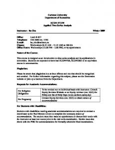
As part of a 4th year capstone design project offered by the Department of Mechanical and Aerospace Engineering at Carleton, the novel 6 DOF Atlas motion platform, pictured in Figure 1, was conceptually designed by the Carleton University Simulator Project (CUSP). The Atlas motion platform provides a unique solution to the problem faced by all motion platforms: providing a realistic sensation of motion within a finite volume of space. The standard Stewart platform is one solution to this problem but is confined to a specific range of rotational motion that is limited not by restrictions of space, but by inherent restrictions of design. Atlas eliminates these restrictions by mounting a spherical cockpit on an orthogonal three-axis gantry upon which three omni-directional wheels (“omni-wheels”) provide unlimited rotational actuation about any axis. This arrangement effectively decouples the orientating and positioning degrees-of-freedom. Thus, the Atlas motion platform offers the potential to increase the motion-fidelity over current simulation platforms, making it ideally suited for ground, marine, and air vehicle simulation platforms; as well as applications in the entertainment industry such as gaming, movie, and amusement park motion platforms. This paper builds upon the kinematic development previously accomplished by Robinson et al [1] and Holland et al [2]. Further analysis of the velocity-level kinematic equations performed in this
Figure 1: Atlas proof-of-concept demonstrator. paper demonstrates that the non-holonomic constraints, due to kinematic slip at the omni-wheelsphere interface, are handled implicitly by the equations. Thus, the kinematic velocity equations can be integrated and differentiated directly to obtain expressions for position and acceleration-level control of the Atlas sphere. Additionally, the dynamic equations of motion are developed that provide the omni-wheel torque values required to produce the desired kinematic angular displacements, velocities, and accelerations.
2
Atlas Platform Architecture
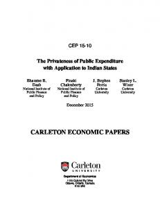
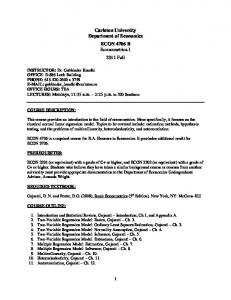
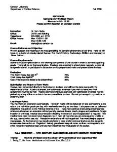
The Atlas motion platform uses a novel structural configuration in order to achieve unlimited rotations about the roll (X-axis), pitch (Y -axis), and yaw (Z-axis) axes or any linear combination of these. This is accomplished by mounting the spherical cockpit on three omni-wheels deployed in an equilateral configuration of 120◦ . A right-handed global coordinate system [X, Y, Z] is fixed to the sphere origin as shown in Figure 2. Thus, omni-wheel deployment lies in the XY -plane with the angle between each identified as β measured counter-clockwise from omni-wheel 1. Each omniwheel is actuated independently by a variable speed DC motor allowing differential speed between each of the omni-wheels and providing the ability to rotate the Atlas sphere 360◦ about any axis. The driving axis of each omni-wheel forms a 40◦ angle upward, identified as α in Figure 3, relative to XY -plane. This configuration optimizes the structural weight of the platform by using the omniwheels for cockpit support and actuation. The equilateral deployment of the omni-wheels provides distribution of the static weight thereby eliminating the need for additional structural components to support the sphere. It also ensures that the DC motors act in parallel to simultaneously apply torque to orient the sphere, and thereby share the load and reduce the size and weight of the motors. These benefits would be lost, however, if the omni-wheels were place on orthogonal axes,
2
Figure 2: Omni-wheel deployment in the XY-plane shown from the bottom view. in which case additional structural components would be required to support the sphere, and larger DC motors would be required to independently actuate the sphere in the pitch, roll and yaw case. The kinematic analysis requires the placement of five coordinate frames at key locations. The first is the global or inertial frame [X, Y, Z] located at the centre of the sphere with the X-axis pointing toward omni-wheel 1 and the Y and Z-axes defined according to the right-hand-rule, see Figure 2. A local reference frame [X 0 , Y 0 , Z 0 ] is placed initially coincident with the inertial frame, but then rotates with the sphere about the sphere origin. Three omni-wheel frames, denoted [xk , yk , zk ] where k ∈ {1, 2, 3} for each omni-wheel, are fixed to the centre of the omni-wheels. The x-axis points outward from the omni-wheel centre along the driving axis and the z-axis points towards the omni-wheel-sphere contact point, see Figure 3. Various parameters that define the dimensions of the Atlas sphere and the optimal deployment of the omni-wheels are not discussed in this paper and will be left as variables. These include the diameter of the sphere and the location of the Atlas sphere’s centre relative to the omni-wheels. For the purpose of analysis, the radius vector of the Atlas sphere will define the position vector of
Figure 3: Omni-wheel coordinate reference frames.
3
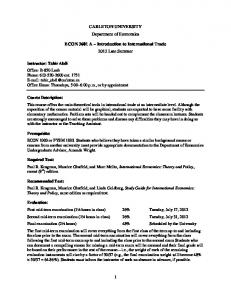
each omni-wheel contact point in the [X, Y, Z] coordinate frame, expressed as Rk , and having the components [RkX , RkY , RkZ ] for each k th omni-wheel. Since R1 is defined as a vector pointing from the origin of the global frame to the omni-wheel 1 contact point it will have a positive X-direction component, a negative Z-direction component, and a zero Y -component as shown in Figure 4. The other two radial vectors for omni-wheels 2 and 3 can be determined using the transformation matrix, Tk , defined by a Z-axis rotation matrix in terms of the omni-wheel positions, βk : c βk s βk 0 Tk = −sβk cβk 0 , (1) 0 0 1 where cβk , and sβk respectively denote cos βk and sin βk , k ∈ {1, 2, 3}. Thus, the general expression for the radial vectors, Rk , for each omni-wheel can be determined as R 1X c β2 R 1 X c β3 R 1 X R1 = 0 ; R2 = −sβ2 R1X ; R3 = −sβ3 R1X . (2) R 1Z R 1Z R 1Z As these position vectors each represent the location of the omni-wheel contact point with respect to the sphere origin then kR1 k = kR2 k = kR3 k = kRk.
Figure 4: Omni-wheel-sphere contact point position vectors.
4
(3)
3
Atlas Kinematics for Spherical Motion Control
The kinematic equations for Atlas angular motion control are derived by considering each degree-offreedom separately and then applying the principle of superposition to obtain the resultant angular motion response of the Atlas sphere. The result is a set of three equations in three variable omniwheel inputs for each level of Atlas kinematic control: displacement, velocity, and acceleration. These equations form a linear combination of omni-wheel angular inputs that produce a resultant sphere angular response about an infinite number of rotation axes.
3.1
Slip Considerations
The Atlas configuration shown in Figure 4 comprises a 3 DOF system with angular input possible about each of the global orthogonal axes in the [X, Y, Z] frame. Because of the Atlas kinematic architecture, each of the three omni-wheels represent an independent angular input that is a coupled rotation about the X, Y , and Z-axes, and induces a corresponding angular response of the sphere, Ωk , k ∈ {1, 2, 3}. This induced angular response is an independent rotation of the sphere about a general axis that is parallel to the corresponding omni-wheel driving axis and coincident with the origin of the global frame. The independence of each sphere angular response is conditional on a well selected omni-wheel location specified by angle θ, that allows each of the three general rotational axes to be resolved along the orthogonal axes of the global frame. For example, a value of θ = 0◦ , would place each omni-wheel in the XY -plane, creating a 1 DOF system, and therefore not satisfy this requirement. Thus, with an appropriate omni-wheel location selected, the resultant angular response of the sphere is formed from the superposition of the independent sphere angular responses according to Ω =
3 X
Ωk .
(4)
k=1
Analysis at each of the three omni-wheel contact points will show that there will typically be a difference between the linear velocity of the omni-wheels and that produced by the resultant response of the Atlas sphere. The difference is produced as a result of superimposing the effects of each of the omni-wheel-induced angular responses to obtain the resultant sphere angular response. This kinematic velocity difference between the linear velocity components at the contact points is referred to as kinematic slip (or simply “slip”) in this paper. Slip occurs in a general path across the omni-wheel sphere contact point and can be resolved into two orthogonal components: a tangential component that is directed along the tractive path of the omni-wheel, and a transverse component directed parallel to the omni-wheel driving axis. Slip as considered in this paper is a different phenomenon than “skid”, which is caused by the loss of traction of the omni-wheel at the sphere contact point. Skid will occur when an excess amount of torque, supplied by the omni-wheel, causes the applied linear force component to exceed the force of friction. For purposes of kinematic development, it will be assumed that the maximum torque that the omni-wheel can supply without loosing traction is known, and therefore the omniwheel torque values are controlled and skidding avoided. In performing the kinematic analysis, each omni-wheel can be considered without regard to the effects of the other two since each omni-wheel represents an independent degree-of-freedom of the system. This implies that the kinematic analysis can be conducted in the absence of slip. Such
5
an assertion is used in the simpler kinematic analysis of a projectile moving in three-dimensional space. Considering a situation where three distinct force components act on the projectile, then in the most general case, each force will induce motion in all three orthogonal X, Y , and Z-directions simultaneously. Resolving the motion components into these three independent orthogonal axes allows the analysis for each direction to be conducted without regard to other two. For example, the kinematics in the X-direction does not depend upon the kinematics of the Y -direction. Superimposing the results of each analysis yields the resultant mathematical description of the projectile’s motion in all three orthogonal directions at once. A similar kinematic analysis can be used for Atlas in order to remove the slip that occurs at the omni-wheel-sphere contact points. Since the angular inputs supplied by the omni-wheels form independent angular rotations about the X, Y , and Z-axes, the kinematic analysis for each omniwheel input can be conducted without consideration for the angular motion effects induced into the sphere by the other two omni-wheels. This assumption implies that each omni-wheel contributes a coupled angular rotation, Ωk , about each of the orthogonal axes of the global frame, [X, Y, Z], in the absence of slip. The final superposition of all three omni-wheel-induced angular responses yields the resultant mathematical description of the angular motion of Atlas in all three orthogonal directions. Such a description inherently includes the kinematic slip at the contact points. Thus, the kinematic slip does not occur until the three solutions are superimposed to obtain the general kinematic description of the sphere’s angular motion in three-dimensional space.
3.2
Velocity-Level Kinematics
The velocity-level kinematics for Atlas rotational control as developed by Robinson et al [1] is summarized here and forms the basis for the development of the position and acceleration kinematic equations. The velocity-level kinematic equations relate the angular velocities of the three omniwheels, ω k , expressed in the omni-wheel reference frames [xk , yk , zk ], k ∈ {1, 2, 3}, to the resulting angular velocity of the Atlas sphere, Ω, expressed in the global-frame [X, Y, Z]. As discussed, the kinematic analysis of each k th omni-wheel can be accomplished without regard to the effects induced by the other two since each represents a single independent input into the 3 DOF system. This allows the construction of the kinematic equations in the absence of slip. However, to obtain the resultant angular velocity of the sphere, the effects of all three omni-wheels must be superimposed. Each omni-wheel produces only a y-component of velocity in the local k th omni-wheel frame supplying a tangential linear velocity to the sphere according to vk = ω k × rk = [0, −vky , 0]T ,
(5)
where ω k = [ωkx , 0, 0]T and rk = [0, 0, rz ]T . For each omni-wheel, the radius vector, rk , is directed from the centre of the omni-wheel axis to the sphere contact point along the z-axis. The omni-wheel linear velocities, vk , are tangent to the Atlas sphere and can be transformed into the global-frame using Equation (1) as follows: Vk = Tk vk .
(6)
This linear velocity produced by omni-wheel k, induces a corresponding angular velocity, Ωk , k ∈ {1, 2, 3} at the k th contact point according to the expression Vk = Ωk × Rk .
6
(7)
The inverse cross product of the above expression relates the angular velocity of the Atlas sphere produced by omni-wheel, k, to the respective linear velocity of the omni-wheel [3]: Ωk =
Rk × Vk . kRk2
(8)
So far, the analysis has focussed only on the contribution of kinematic motion from a single omni-wheel, k. As this is a linear system, the sphere angular velocities produced by each individual omni-wheel can be superimposed to gain the resultant sphere angular velocity, Ω, according to Ω =
3 X
Ωk .
(9)
k=1
As previously discussed, each omni-wheel contributes a component of the total sphere angular velocity about the global-axes [X, Y, Z]. Superimposing each component forms a vector of angular velocity contributions for each omni-wheel that when summed produces the resultant Atlas sphere angular velocity which necessarily includes tangential and transverse components of slip across the omni-wheel-sphere contact points. This result is explicitly expressed when the Atlas Jacobian, J, is extracted from Equation (9) to produce the final velocity-level kinematic equation R 1Z R 1Z c β2 R 1 Z c β3 ω1 rz 0 −R1Z sβ2 −R1Z sβ3 ω2 . Ω = Jω = (10) kRk2 −R1X −R1X −R1X ω3 The expression represents a linear combination of the individual omni-wheel angular velocities in the [xk , yk , zk ] frame, and transforms them into the resultant Atlas sphere angular velocities in the [X, Y, Z] frame. Examination of the Jacobian shows that it is always invertible for any configuration provided that the initial design parameters do not result in architectural singularities [1]. This permits the inverse problem of determining the required omni-wheel velocities given a desired sphere angular velocity by simply taking the inverse of the Jacobian and multiplying both sides to produce ω = J−1 Ω. (11) As discussed, Equation (10) includes the kinematic slip components created at the omni-wheelsphere contact points. However, these components can be extracted by using the slip model developed by Holland et al [2]. This exercise is left to the interested reader for further exploration.
3.3
Position and Acceleration-Level Kinematics
The determination of the position and acceleration kinematic equations becomes a trivial task since the velocity kinematic Equation (10) can be directly integrated or differentiated with respect to time. This is because the Jacobian, J, consists entirely of time invariant geometric elements that define the dimensions of the sphere and the angular deployment of the omni-wheels. Once these are defined, they do not change with time and thus the Jacobian remains constant during integration and differentiation.
7
Integrating Equation (10) with respect to time yields the expression for position-level kinematics:
Θ = Jθ =
R1Z rz 0 kRk2 −R1X
R 1 Z c β2 −R1Z sβ2 −R1X
R 1Z c β3 θ1 −R1Z sβ3 θ2 , −R1X θ3
(12)
which describes linear combinations of angular displacements, θ k , for each omni-wheel, k ∈ {1, 2, 3}, and superimposes the components into the overall angular displacement of the Atlas sphere, Θ, in the global-frame [X, Y, Z]. Differentiating Equation (10) with respect to time yields the expression for acceleration-level kinematics: R 1Z R 1Z c β2 R 1Z c β3 α1 rz 0 −R1Z sβ2 −R1Z sβ3 α2 , (13) A = Jα = kRk2 −R1X −R1X −R1X α3 which forms a linear combination angular accelerations, αk , for each omni-wheel, k ∈ {1, 2, 3}, and superimposes the components into the overall angular acceleration of the Atlas sphere, A, in the global-frame [X, Y, Z]. Again, as for velocity-level kinematics, the angular displacement and acceleration slip components are accounted for implicitly by superimposing the individual effects of each omni-wheel.
4
Atlas Dynamics for Spherical Motion Control
The final step in controlling the Atlas rotational motion involves the determination of the torque required for the omni-wheels to generate the desired sphere angular velocities and accelerations. Since we are now dealing with the forces that cause the motion, the kinematic equations developed for angular position, velocity, and acceleration will be used together with the mass properties of the Atlas sphere in order to determine the dynamic equations of motion.
4.1
Atlas Mass Properties and Frame Transformations
The primary mass property considered for rotational motion is the inertia tensor, I, defined as IXX −IXY −IXZ −IY Z . I = −IY X IY Y (14) −IZX −IZY IZZ However, if the local frame [X 0 , Y 0 , Z 0 ] which rotates with the sphere is used, the products of inertia all become zero leaving only the moments of inertia along the diagonal. IXX 0 0 0 IY Y 0 0 . I = 0 (15) 0 0 IZZ 0 Since the kinematic equations produce angular velocities and accelerations of the sphere in the global frame, these values must now be transferred into the local frame. This can be accomplished
8
with the position-level kinematics expression which provides the orientation of the sphere, and hence the local frame rotating with it, at any moment in time. Once the angles of rotation of the local frame have been determined, a rotation matrix for each of the three angles can be formed which represent a rotation of the local frame with respect to the global frame about each of the global axes X, Y , and Z: 1 0 0 G 0 cΘX −sΘX , L RX (ΘX ) = 0 sΘX cΘX cΘY 0 sΘY G 0 1 0 , (16) L RY (ΘY ) = −sΘY 0 cΘY cΘZ −sΘZ 0 G sΘZ cΘZ 0 . L RZ (ΘZ ) = 0 0 1 Multiplying these three rotation matrices together produces the overall orientation of the local frame with respect to the global frame. It should be noted that the order of multiplying the matrices must be maintained since matrix multiplication is generally not commutative, nor are rotations [4]. G L RXY Z (ΘX , ΘY , ΘZ )
G G =G L RZ (ΘZ )L RY (ΘY )L RX (ΘX )
(17)
−1 The inverse of the above rotation matrix, G L RXY Z , provides the orientation of the global axes with respect to the local axes and can be used to map the global values of angular velocity and acceleration into the local frame. The following two expressions demonstrate how this is accomplished: L
−1 G Ω=G L RXY Z Ω,
(18)
G −1 G L RXY Z A,
(19)
L
A=
where G Ω and G A are the global sphere angular velocity and acceleration required for simulation and L Ω and L A are the mapped local angular velocity and acceleration.
4.2
Omni-Wheel Torque Actuation
Now that all the necessary components are in the local frame, Euler’s equations of motion can be used to compute the moments about the local-axes and are determined to be [5] 0 0 MX = IX Λ0X − (IY0 − IZ0 )Ω0Y Ω0Z , 0 MY0 = IY0 Λ0Y − (IZ0 − IX )Ω0Z Ω0X ,
MZ0
=
IZ0 Λ0Z
−
0 (IX
−
(20)
IY0 )Ω0X Ω0Y .
Collecting these terms into the vector, M0 , the moments must be transformed back into the global frame using Equation (17) producing, M, the moments expressed in the global frame. Finally, the torque for each omni-wheel can be determined using the Jocobian again to relate the moments about the global [X, Y, Z] axes to each of the k th omni-wheel frames [xk , yk , zk ], where k ∈ {1, 2, 3}: T = JT M,
9
(21)
where T is the collection of torque values required by each omni-wheel, k, to produce the moments, M, about the global axes.
5
Conclusions
The Atlas motion platform achieves unlimited angular motion about any axis using three omniwheels that induce simultaneous, but independent, angular displacements in the Atlas sphere. As each omni-wheel rotates, the angular inputs are superimposed yielding the resultant angular response of the sphere. The resultant response must necessarily produces slip in the tangential and transverse directions at the omni-wheel-sphere contact points. However, since each of the omni-wheels represents an independent input into the the 3 DOF system, each omni-wheel can be analyzed independently from the angular effect produced by the other two. Therefore, explicit determination of the slip components, while possible, is not necessary for a complete kinematic analysis of the Atlas motion platform. The velocity kinematics expression can be directly integrated to obtain the position-level kinematics or differentiated to obtain the acceleration-level kinematics. Using these kinematic expressions and the mass properties of the sphere, the dynamic torque values necessary to induce the required angular velocities and accelerations can be determined. The position kinematic expression is used to track the orientation of the sphere and produce the transformation matrices required to map the angular velocities and accelerations into the local frame from the global frame and vice versa. Using the local frame causes the products of inertia to cancel and allows Euler’s equation of motion to be used to determine the required moments that must be induced in the sphere by the omni-wheels.
References [1] J. Robinson, J.B. Holland, M.J.D. Hayes, and R.L. Langlois. “Velocity Level Control of a Spherical Orienting Device Using Omni-directional Wheels”. 2nd CCToMM Symposium on Machines, Mechanisms and Mechtronics, Canadian Space Agency, on CD, May 26-27, 2005. [2] J.B. Holland, M.J.D. Hayes, and R.G. Langlois. “Slip Model for the Spherical Actuation of the Atlas Motion Platform”. CCToMM Symposium on Machines, Mechanisms and Mechtronics, Canadian Space Agency, on CD, May 26-27, 2005. [3] J. Angeles. Cross-Product Inversion. private communication, August 25, 2004. [4] J. Craig. Introduction to Robotics: Mechanics and Control. Pearson - Prentice Hall, third edition, 2005. [5] R.C. Hibbeler. Engineering Mechanics: Statics & Dynamics. Prentice-Hall, ninth edition, 2001.
10