The basic equations of continuum mechanics are the balance equations. .... the Avrami equation is a special case of the Schneider rate equations as shown.
A computational model for processing of semi-crystalline polymers: The effects of flow-induced crystallization Gerrit W.M. Peters Materials Technology (www.mate.tue.nl), Dutch Polymer Institute, Eindhoven University of Technology, P.O. Box 513, 5600 MB Eindhoven, The Netherlands,
Abstract. A computational model for the combined processes of quiescent and flowinduced crystallization of polymers is presented. This modelling should provide the necessary input data, in terms of the structure distribution in a product, for the prediction of mechanical properties and shape- and dimensional-stability. Rather then the shear rate as the driving force, a viscoelastic approach is proposed, where the viscoelastic stress (or the equivalent recoverable strain) with the highest relaxation time, a measure for the molecular orientation and stretch of the high end tail molecules, is the driving force for flow induced crystallization. Thus, the focus is on the polymer that experiences the flow, rather then on the flow itself. Results are presented for shear flow, extensional flow and for injection moulding conditions of an isotactic Polypropylene (iPP).
1
Introduction
The resulting local properties of a product made of semi-crystalline polymers strongly depend on the crystalline structure which is determined by both molecular properties and the processing conditions applied, i.e. the thermal-mechanical history experienced by the polymer in the process. Consequently, this thermalmechanical history (e.g. in injection moulding, film blowing or fiber spinning) has to be modelled in order to describe nucleation and crystallization kinetics and their dependence on flow-induced structure formation. Experimental results in the literature show that flow-induced crystallization correlates with the viscoelastic stresses, much more than with the macroscopic strain or strain rate, leading to the conclusion that chain orientation/extension is the governing phenomenon. The orientation of polymer chains can result in the development of anisotropic structures which influence the mechanical properties and the dimensional stability, i.e warpage and (anisotropic) shrinkage. A modelling tool is needed to prevent and correct for such unwanted properties and phenomena. The ultimate goal is to develop a tool that is able to improve or even optimize polymer synthesis and industrial processes. However, several of the underlying relations are still not clear due to the complex mutual interaction of many parameters. Therefore, optimization of properties in industry is still done by expensive and time consuming trial and error methods, which -at best- are based on cumulative experience.
2
Gerrit W.M. Peters
The need for such a modelling tool became even more urgent since the development of novel metallocene-based catalysis. Compared to conventional ZieglerNatta catalysis, metallocene-based polymers are much more well defined and possess a narrow molecular weight distribution. Moreover, differences in regularity of the polymer chains exist caused by sterical restrictions during polymer synthesis [1]. The relation between molecular properties, processing conditions and final properties that result from the micro-structure formed, can be determined once recent developments in detailed modelling are condensed into constitutive equations that are the input of continuum mechanical modelling. The relation between molecular weight distribution and linear viscoelastic properties [2,3] and that between rheology and flow-induced nucleation [4,5] has now become much more clear. Polymer rheology can at present quantitatively be described with the (extended) Pom-Pom model [6–8]. Consequently, a powerful tool could be obtained once these methods are combined to model the whole life cycle of a polymer: from the synthesis to properties via processing. However, much more advanced experimental methods and set-ups than used at present have to be developed to be able to validate the modelling and to obtain the required input parameters.
2 2.1
Modelling Balance equations
The basic equations of continuum mechanics are the balance equations. In their local form, the equations for mass, momentum, moment of momentum and energy read, respectively: ρ˙ + ρ∇.v = 0
(1)
∇.σ c + ρf = ρv˙
(2)
σ=σ
c
ρe˙ = σ : D − ∇.h + ρrh
(3) (4)
in which v the velocity, ρ the density, σ the Cauchy stress tensor, f the specific body force, e the internal energy, h the heat flux vector and rh the specific heat source. In the following, constitutive relations will be presented for the stress and the density in terms of the kinetics of the different phases. Details on constitutive models for the other quantities, such as internal energy and heat flux can be found in literature, see for example [5]. 2.2
Constitutive equations
Viscoelastic stress A general expression for the evolution of the Cauchy stress tensor σ is given by [9] �
σ + A · σ + σ · Ac = O
(5)
Flow-induced crystallization of polymers
3
where A is the slip tensor (also known as the plastic deformation rate tensor Dp ) which takes into account the non-affine deformation of the molecules and the upper convective derivative of the Cauchy stress tensor is defined by �
σ= σ˙ − L · σ − σ · LT
(6)
The Cauchy stress σ is related to the recoverable strain tensor Be according to (7)
σ = GBe
in which G is the elastic modulus. Once the viscoelastic stress is known, the recoverable strain is also defined by Eq.(7). With the definition of the extra stress tensor τ = G(σ − I) and the upper convective derivative of the unity �
tensor I = −2D, it follows �
τ + A · τ + τ · Ac + G(A + Ac ) = 2GD
(8)
For a realistic description of melt behavior a multi-mode model has to be used: σ = −pI +
n �
τi
(9)
i=1
Most known models are captured within the following definition of the slip tensor A = α1 σ + α2 σ −1 + α3 I
(10)
by a certain choice for the parameters α1 , α2 and α3 . They are given for the Upper Convected Maxwell model (as an example: it is the most simple model for viscoelastic stress) the Leonov model and the extended Pom-Pom model in Table 1. Table 1. Definition of the slip tensor for the upper convected Maxwell (UCM), the Leonov and the Extended Pom-Pom model (taken from [8,10]).
Model
α1
α2
α3
Ref.
UCM
0
G − 2λ
1 2λ
[10]
Leonov
1 4Gλ
G − 4λ
Extended Pom-Pom
α 2Gλ
− G(1−α) 2λ
−
Iσ −G2 Iσ −1 12Gλ 1 2λg
[10] [8]
4
Gerrit W.M. Peters
The Extended Pom-Pom model has a generalized relaxation time λg defined by � � 1 1−α αIσ·σ 2 (11) 1 − = − + λ−1 g λ0b Λ2 3G2 λ0b Λ2 λs Λ with a material parameter α, which defines the amount of anisotropy in molecular friction and (Brownian) motion (i.e. reptation) and the molecular stretch Λ. Two different relaxation times are defined, namely the relaxation time of the backbone orientation λ0b and the backbone stretch λs . Slip tensors for some other, well known constitutive equations can be found in [9,10]. The upper convected Maxwell (UCM) model can describe different aspects of linear and non-linear viscoelastic behavior of a polymeric fluid by using multi modes. Linear behavior can be predicted accurately, while the non-linear viscoelastic regime is only described qualitatively. It can predict a first normal stress difference in shear, strain hardening in elongation and stress relaxation after cessation of flow. However, shear viscosity and the first normal stress difference are predicted to be independent of shear rate, and extensional viscosity can become infinite for finite extensional rates [12]. The differential equation of the UCM model is given by �
τ +
1 τ = 2GD λ
(12)
The UCM model is fully determined using linear viscoelastic data only. The Leonov model can describe the (non)-linear viscoelastic behavior of a polymeric liquid in shear rather well by using multi modes. Elongation is poorly described [12]. The differential equation of the Leonov model is given by � 1 1 1 � τ + τ+ I(τ +GI) − G2 I(τ +GI)−1 (τ + GI) = 2GD τ ·τ − λ 2Gλ 6Gλ � ��
�
(13)
(a)
The Leonov model is, like the UCM model, determined by the linear viscoelastic data only. For incompressible, planar deformations part (a) of Eq. (13) is equal to zero. The Leonov model is in this case equivalent to the Giesekus model with the parameter α in the Giesekus model equal to 0.5. The Pom-Pom model was proposed by McLeish and Larson [7]. It describes the strain hardening in elongation and thinning behavior in shear for branched polymers. They defined an idealized molecule, the ’pompom’, which consists of a backbone with a number of branches at each end. A key feature in this model is the separation of stretch and orientation of a polymer molecule. Verbeeten et al. [8] proposed an extended version of the model which also predicts a second normal stress difference. Excellent quantitative agreement with measurements of branched (LDPE) and linear polymers (HDPE) was found by using a multi mode version. The extended Pom-Pom model is given by �
τ + λ(τ )−1 · τ = 2GD
(14)
Flow-induced crystallization of polymers
with inverse relaxation tensor
� � � 1 α 1 1 λ(τ )−1 = τ+ I+G − 1 τ −1 λ0b G f (τ ) f (τ ) �� �
5
(15)
(a)
and extra function f (τ ) defined via � � � � 1 αIτ ·τ 1 1 2 1− 1− + = λ0b f (τ ) λs Λ λ0b Λ2 3G2 � �� � �� (b)
(16)
(c)
Backbone stretch and stretch relaxation time are defined as Iτ Λ= 1+ , λs = λ0s exp(−ν(Λ − 1)), 3G0
ν=
2 q
(17)
in which q is the number of branches. Parameter α (α ≥ 0) describes a Giesekus type of anisotropy [13]. This parameter influences the second normal stress difference only. The Extended Pom-Pom model is equivalent to the original (approximative) Pom-Pom model for α = 0. The orientation relaxation times of the backbone λ0b are obtained from linear viscoelastic data. The number of branches q, the stretch relaxation times λs and the anisotropy parameter α have to be determined for each mode. This large number of parameters seems to be a drawback. A physical guideline related to the structure of the Pom-Pom molecule can be taken into account. The free ends of the molecule correspond to fast relaxation times and no or less branches. Towards the center of the molecule, relaxation and branches will increase. Moreover, the stretch relaxation time is constrained in the interval λ0b,i−1 < λ0s,i ≤ λ0b,i . Stretch and orientation are gathered in one equation in the extended PomPom model. In case of α = 0 two situations can be distinguished: • Only orientation relaxation for low strains (Λ ≈ 1; part (a) and (b) of Eqs. (15) and (16) are equal to zero.) • Only stretch relaxation for high strains (Λ >> 1; part (c) of Equation(16) is equal to zero.) Verbeeten [8] showed that the described parameter trends are obtained automatically using a non-linear fitting procedure. Crystallization Non-isothermal crystallization of spherulites is described by the Schneider’s rate equations [14,15], a set of differential equations, which give the structure developing for quiescent conditions. Mean number of spherulites and their mean radius, surface and volume are calculated from: φ3 = 8πα φ2 = Gφ3
(φ3 = 8πN ) (φ2 = 8πRtot )
�
rate� � radius�
(18) (19)
6
Gerrit W.M. Peters
φ1 = Gφ2 φ0 = Gφ1 φ0 = − ln(1 − ξg )
(φ1 = Stot ) (φ0 = Vtot )
�
surf ace� � volume� � spacef illing �
(20) (21) (22)
with the nucleation rate α and the growth rate G. Impingement of the spherulites is captured by an Avrami model, Eq. (22). The morphology is described per unit volume by the total volume of spherulites Vtot , their total surface Stot , the sum of their radii Rtot and the number of nuclei N. The relation of these parameters with ψi is given between brackets. The number of nuclei and the growth rate have to be measured as a function of temperature. The very often used Avrami equation (22), which describes space filling in case of isothermal crystallization for which all nuclei appear at t0 and where the growth rate is constant for t > t0 , is given by �
4π (23) ξg = 1 − exp − N G3 (t − t0 )3 3 with t0 the time that the crystallization temperature was reached. Notice that the Avrami equation is a special case of the Schneider rate equations as shown in [4]. For flow-induced nucleation and crystallization Zuidema et al. [5,16] proposed a modification (SJ2 -model) for the shear-induced crystallization model of Eder and Janeschitz-Kriegl [4], which gave a good description of the flow-induced structures obtained in their experiments. Zuidema et al. used the recoverable strain modelled with a Leonov type of model as a driving force for flow-induced crystallization. It was demonstrated that the flow-induced structure correlated most strongly with the viscoelastic mode with the highest relaxation time. Therefore, only the second invariant of the deviatoric part of the recoverable strain ¯ d ) = 1/2 B ¯d : B ¯ d ) corresponding with the maximum rheological relax(J2 (B e e e ation time was used. This invariant is a measure for the molecular orientation [12]. With the SJ2 -model, non-isothermal crystallization of cylindrical structures (which are for convenience called shish-kebabs) can be described. It has the same structure of differential equations as the Schneider rate equations. Mean number of shish-kebabs and their mean length, surface and volume are calculated from: ψ3 = ψ˙ 3 + τn ψ2 = ψ˙ 2 + τl = ψ˙ 1 ˙ = ψ0 ψ0
8πJ2 gn� ψ 3 J2
gl� gn�
Gψ2 Gψ1 = − ln(1 − ξg )
(ψ3 = 8πNf ) (ψ2 = 4πLtot ) (ψ1 = Stot ) (ψ0 = Vtot )
�
rate�
(24)
�
(25)
length�
�
surf ace� � volume� � spacef illing �
(26) (27) (28)
with the driving force J2 , the growth rate G, the scaling factors gn� and gl� to describe the sensitivity of the flow-induced nuclei and length on J2 , and the
Flow-induced crystallization of polymers
7
characteristic times τn and τl to describe the relaxation behavior of the flowinduced nuclei and length. Impingement of the cylindrical structures is captured by an Avrami model, Eq. (28). The morphology is described per unit volume by the total volume of shish-kebabs Vtot , their total surface Stot , the sum of their lengths Ltot and the number of flow-induced nuclei Nf . The relation of these parameters with ψi is given between brackets. Eder’s rate equations are obtained by replacing J2 by a scaled value of the shear rate squared. Molecular orientation will generate extra nuclei, Eq.(24). When the orientation is strong enough, these nuclei can grow in one direction, Eq. (25). The radial growth rate of the cylindrical structures is taken equal to the spherulitical growth rate. Of course, other choices for the radial growth dependent on J2 are possible. The relaxation time τl is in general taken very large, because reduction of length can only occur via melting. Zuidema [5,16] considered nucleation to act as physical cross-linking. Consequently, an increased number of nuclei causes an increase in the rheological relaxation time. A simple, linear relationship between flow-induced nuclei and the highest rheological relaxation time was chosen.
λmax
� � βNf = aT (T )λ0,max 1 + � gn
(29)
with λ0,max the highest rheological relaxation time at a reference temperature, aT the shift factor and β a scaling factor that describes the interaction between nuclei and rheology. Consequently, the scaling factors β, gn� and gl� should be measured as a function of flow conditions. The concept of the equivalence of physical cross-linking and nucleation in the Leonov model can be used in the Pom-Pom model in rather natural way. Increase in the number of nuclei gives an increase in the number of branches and relaxation time. This means that the scaling factor β in Equation(29) is related to the number of branches in the Pom-Pom model. In the case of flow, both spherulitical and flow-induced structures contribute to the degree of space filling, depending on the influence of J2 . The Avrami model for impingement is then described by φ0 + ψ0 = − ln(1 − ξg )
(30)
There are two big advantages when applying the Pom-Pom model to the linear polymers used in this study. First, both elongation and shear data can be described excellent with the same set of fitting parameters. Second, the physical description that serves as a basis for this model (i.e. the Pom-Pom molecule) results in a more transparent model. The physical cross-linking process, as proposed by Zuidema et al. [5,16], can be related to the increase in the number of branches during crystallization.
8
Gerrit W.M. Peters
3
Results
0.1
0.2
0.09
0.18
0.08
0.16
0.07
0.14
0.06
0.12
thickness [mm]
thickness [mm]
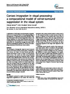
The most important features of the model will be demonstrated by some illustrative examples. A more extensive treatment of these results can be found in [5,16] and [17]. Zuidema [5,16] predicted the position of the transitions of different flow induced layers in a slit flow as measured by Jerschow [18]. He considered only shear flows and, therefore, used the Leonov model for viscoelastic modelling since this model gives an excellent description of viscoelastic shear data. Postulating that variables describing the flow induced structure should be the same at these transitions, and determining the values from one independent experiment, he could reproduce the transition position for a broad range of deformations (two different wall shear rates, many different shear times). Fig. (1) shows the position of
0.05 0.04
0.1 0.08
0.03
0.06
0.02
0.04
0.01
0.02
0
0
5
shear time [s]
10
15
0
0
5
shear time [s]
10
15
∗
Fig. 1. Measured ( ) thickness of the boundary of the flow-induced layer for different shear times (from [18]), together with the numerically determined position of this boundary (solid line) for a wall shear rate of 79 (left) and 115 [s−1 ] (right).
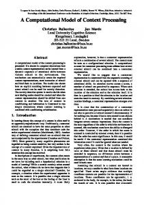
the transition between the highly oriented layer near the duct wall and the fine grained layer next to it. Predictions are within the experimental scatter. Next, it was demonstrated that the model could predict qualitatively (for most materials used in literature the required data set is missing) a wide range of observations on flow induced crystallization as reported in literature. Two examples are given here. In Fig. (2) shows for a continuous, isothermal shear flow at different, constant shear rates the induction time, the time that a noticeable rise in the viscosity is found [19]. The induction time decreases dramatically if some critical shear rate is exceeded. Although the data set of a different iPP (Daplen KS10, Borealis) was used in the numerical simulations, the same behavior as with the experiments is found. Vleeshouwers and Meijer [20] used three iPP’s with different molar mass distribution in their experiments. After a well defined shear treatment of the melt, using a cone and plate configuration, at an elevated temperature, and a
Flow-induced crystallization of polymers
9
2
induction time [s]
10
1
10
0
10 −1 10
0
10
−1 shear rate [s ]
1
10
Fig. 2. The calculated induction time using parameters of the iPP Daplen KS10 (Borealis). Measurements ( ) after Lagasse [19].
�
subsequent quench to the crystallization temperature, the storage (G ) and loss �� modulus (G ) were monitored. The rise in the moduli was used to determinethe the induction time. Experiments at a constant total shear treatment showed that increasing the shear rate (and consequently decreasing the shear time) lowers the induction time (fig. 3, right). Using the data for the iPP Daplen KS10, Borealis, crystallization kinetics are calculated, using a temperature profile that resembles the one Vleeshouwers [20] used, and induction times are calculated for a constant total shear of γ = 250[−]. Results are given in fig. 3. The model confirms the experimental observations in a qualitattive way. The measurements indicate the presence of a plateau region at low shear times. This probably is related to the difference in startup behavior of the materials. The experiments with a constant shear rate during various shear times show a strong decrease in induction time in the low total strain region (low shear times), while in the high total strain region (high shear times) the induction time decreases much more gradually. Again, the calculated induction times confirm this observation in a qualitative way. Swartjes [17] studied extensional flows and, therefore, he used also the PomPom model since this model is superior in describing both, shear and extensional rheological behavior. A special cross-slot flow cell was developed enabling birefringence and time resolved WAXS measurements, see Fig. 4. To create a flow, an outer ring with two cams is rotated. Measurements and numerical results relate to the central part (2x2 mm) of the flow cell where around the stagnation point a planar elongational flow is present. One of the major outcomes, both, experimentally and numerically, was a highly oriented narrow strand (≈ 80 µm) of a fibre-like crystalline structure around the outflow centerline that developed at a relatively high temperature of ≈ 149o C, a temperature at which noticeable quiescent crystallization effect takes hours. This is shown in Figure (5), where the integrated WAXS intensity is given for the (110) refection as a function of the azimuth angle and the position
10
Gerrit W.M. Peters 400
2000
350 shear = C
300
induction time [s]
induction time [s]
1500
shear = C
250
rate = C
200
1000
150
500
0
50
100
shear time [s]
150
200
100
250
0
50
100
150 shear time [s]
200
250
300
Fig. 3. Left: measured induction time for a constant shear rate (γ˙ = 5[s−1 ]) and different shear times (•) and the induction time for a constant total shear (γ = 250[−]) and different shear rates ( ) (after [20]). Right: the corresponding predicted induction times (-: SJ2 model, - -: Eder model).
�
2
5
100 130
Fig. 4. Main dimensions in mm of the cross-slot flow cell.
perpendicular (y-coordinate) and parallel (x-coordinate) to the outflow direction. These results were obtained with the micro-focus-beam-line ID13 (beam size 30 µm ) at the European Synchroton Radiation Facility (ESRF). From numerical simulations a qualitatively similar result was found, see Fig. 6, which shows the computed flow-induced mean space filling (the flow is essentially three dimensional) in the cross-slot flow cell. For symmetry reasons, only a quarter of the central area of the flow cell is shown. A very sharp, highly crystalline, narrow band is found also with the numerical simulations. Taking a level of 20% space filling as a threshold, the band has a width in the order of 100 µm. Finally, some examples of predicted structure distributions for injection moulding flows are presented. With injection moulding a cold mould is filled at high speed during which a solidified layer is growing from the wall. At the transition from this solidifying layer to the melt, the relaxation times of the melt become rather high, strongly increasing the effect of the flow gradients on the crystal-
Flow-induced crystallization of polymers 14000 12000
10000
Intensity [a.u.]
Intensity [a.u.]
12000
11
8000 6000 4000 0.4
10000 8000 6000 4000 0.1
0.2
0.05 0
0
−0.2
y [mm]
−0.4
270
360
90
180
0
−0.05
x [mm]
χ [degrees]
−0.1
360
270
180
90
0
χ [degrees]
Fig. 5. WAXS intensity for the (110) reflection vs azimuthal angle and position on the inflow center line (left) and on the outflow center line (right).
0.6
g
mean(ξ ) [−]
0.8
0.4 0.2 0 1
1 0.5
0.5 y [mm]
0 0
x [mm]
Fig. 6. Predicted mean flow induced space filling as a function of the position.
lization behavior. At the free surface of the progressing polymer (the flow front) hot material from the core moves towards the cold walls, experiences a complex deformation history and is cooled rapidly when it reaches the wall. These combined flow phenomena can create rather complex structure distributions in the sample. For example, sometimes a double oriented layer is found with an un-oriented, fine-grained spherulitical layer in between, see Fig. 7. Results for two processing conditions of molding of iPP are compared. Figs. 8 and 9 show the specific total shish length and the specific total amount of oriented material at three different locations in a rectangular mold. The difference between the two simulations is the injection speed. The lower injection speed, Fig. 9, generates a two layer configuration, similar to what is seen in Fig. 7, that varies along the mold cavity. A more extended set of results, based on a varying different processing parameters can be found in [5].
4
Conclusions
A computational model for the simulation of flow induced nucleation and crystallization is presented. The model gives a detailed description of both, quiescent
12
Gerrit W.M. Peters
Fig. 7. Microscopic structure of cross-section near surface (left side of cross section) of 1 mm injection molded plate. Showing the ‘skin layers’ (A), ‘transition layer’ (B), ‘shear layer’ (C) and ‘fine grained layer’ (D).
20
1
10
0.5
10
10
0
0
0.5
1
Total shish length
10
10
0
10
0
0.5
1
1.5 −3
x 10
20
10
10
0
0.5
1
1.5 −3
x 10
1
0.5
0
0
0.5
1
1.5 −3
x 10
1
0.5
10
0
10
0
1.5 −3
x 10
20
10
Volume percentage [−]
10
0
0.5
Thickness [m]
1
1.5 −3
x 10
0
0
0.5
Thickness [m]
1
1.5 −3
x 10
Fig. 8. The distribution of the flow-induced oriented structure across the thickness of the injection moulded product close to the gate (top), far from the gate (bottom) and in between (middle). . Processing conditions: Tinj = 430K, Q = 4.65 10−4 m3 s−1 , Twall = 393K. Left side: total shish-length, right side: volume percentage oriented material.
and flow-induced crystallization for any thermal-mechanical history. The advantage of the use of this model is the dependence of nucleation rate and growth on a (molecular) strain measure rather than the macroscopic shear rate. Improvements or other dependencies can be easily inserted (for example a deformation depended growth rate). The dependence of rheology on nucleation is described by physical cross-links (Leonov) or an enhanced number of branches (Pom-Pom), resulting in an increased relaxation time. The sensitivity of this relation between number of nuclei and rheological relaxation time has to be measured. For comparison with experiments an extended set of material parameters is required. The lack of (part of ) these data is the reason that until now most of the comparisons are still of qualitative nature. A more quantitative comparison is needed for validation and, if necessary, improvement of the model.
Flow-induced crystallization of polymers 20
1
10
0.5
10
10
0
0
0.5
1
Total shish length
10
10
0
10
0
0.5
1
1.5 −3
x 10
20
10
10
0
0.5
1
1.5 −3
x 10
1
0.5
0
0
0.5
1
1.5 −3
x 10
1
0.5
10
0
10
0
1.5 −3
x 10
20
10
Volume percentage [−]
10
13
0
0.5
Thickness [m]
1
1.5 −3
x 10
0
0
0.5
Thickness [m]
1
1.5 −3
x 10
Fig. 9. The distribution of the flow-induced oriented structure across the thickness of the injection moulded product close to the gate (top), far from the gate (bottom) and in between (middle). Processing conditions: Tinj = 430K, Q = 1.16 10−4 m3 s−1 , Twall = 393K. Left side: total shish-length, right side: volume percentage oriented material.
References 1. M. Gahleitner, C. Bachner, E. Ratajski and G. Rohaczek: J. Appl. Pol. Sci., 73 (1999) 2. D.W. Mead: J. Rheology, 38, 6 (1994) 3. C. Pattamaprom, R.G. Larson and T.J. van Dyke: Rheol. Acta, 39 (2000) 4. G. Eder and H. Janeschitz-Kriegl, In: Materials Science and Technology: A Comprehensive Treatment: Processing of Polymers, 18, ed. by H.E.H Meijer, Crystallization, (VCH, Weinheim 1997) pp 269–342 5. H. Zuidema, Flow induced crystallization of polymers. Application to injection moulding, PhD Thesis, Eindhoven University of Technology, The Netherlands (2000) 6. N.J. Inkson, T.C.B. McLeish, O.G Harlen and D.J. Groves: Modelling the rheology of low density polyethylene in shear and extension with the multi-modal Pom-Pom constitutive equation, Proc. PPS 15, ’s Hertogenbosch, the Netherlands (1999) 7. T.C.B. McLeish and R.G. Larson: J. Rheol., 42, 1 (1998) 8. W.H.M. Verbeeten, G.W.M. Peters and F.P.T. Baaijens: J. Rheol., 45, 4, (2001) 9. G.W.M. Peters, Thermorheological modelling of viscoelastic materials, In: IUTAM Symposium on Numerical Simulation of Non-Isothermal Flow of Viscoelastic Liquids: Fluid Mechanics and its Applications, Proc. IUTAM Symposium, Kerkrade, The Netherlands, 1-3 November 1993, ed. by J.F. Dijksman and G.D.C. Kuiken, (Kluwer Academic Publishers 1995), 28, pp 21-35 10. G.W.M. Peters and F.P.T. Baaijens: J. Non-Newt. Fluid Mech., 68 (1997) 11. W.H.M. Verbeeten, Computational Polymer Melt Rheolgy, PhD Thesis, Eindhoven University of Technology, The Netherlands (2001) 12. R.G. Larson, Constitutive Equations for Polymer Melts and Solutions (Butterworths, London 1988) 13. R.B. Bird, C.F¿ Curtiss, R.C. Armstrong and O. Hassager, Dynamics of Polymeric Liquids (John Wiley and Sons, New York 1987) 14. W. Schneider, J. Berger and A. K¨ oppl, In: Physico-Chemical Issues in Polymers, Non-isothermal crystallization of polymers: Application of Rate Equations, (Technomic Publ. Co 1993), pp 1043-1054
14
Gerrit W.M. Peters
15. W. Schneider, A. K¨ oppl and J. Berger: Int. Pol. Proc. II, 3 (1988) 16. H. Zuidema, G.W.M. Peters and H.E.H. Meijer, Macromol.Theory and Simulations, 10, 5, (2001) 17. F.H.M.S. Swartjes, Stress Induced Crystallization in Elongational Flow, PhD Thesis, Eindhoven University of Technology, The Netherlands (2001) 18. P. Jerschow, Crystallization of polypropylene. New experiments, evaluation methods and choice of material compositions, PhD Thesis, Johannes Kepler Universit, Linz, Austria (1994) 19. R.R. Lagasse and B. Maxwell: Pol. Eng. Sci., 3, 16 (1976) 20. S. Vleeshouwers and H.E.H. Meijer: Rheol. Acta, 35 (1996)