A computational model of the motion after-effect - UCL

A computational model of the motion after-effect Student: Martin O'Reilly; Supervisors: Alan Johnston and Peter McOwan

Abstract The motion after-effect (MAE) is a phenomenon in which prolonged viewing of a moving stimulus results in the perception of illusory motion in the opposite direction. The MAE is believed to be caused by adaptation of motion sensitive neurons in the brain. The MAE comes two forms. In the static MAE the post-adaptation stimulus is a static pattern. In the dynamic MAE the postadaptation stimulus is a pattern containing balanced motion cues. Examples of dynamic stimuli include flickering gratings; random visual noise (such as the static on a television); and patterns of dots moving in random directions. A model of motion adaptation proposed by van de Grind et al (2003) has been demonstrated to produce a dynamic MAE that fits well with the psychophysical data on the effect. However, to the author's knowledge, this model has yet to be demonstrated to generate a static MAE. This study incorporates this model of adaptation into two of the standard models of mammalian vision (the gradient model and the motion energy model) to determine if it can produce a static MAE and, if it does, how well it corresponds to the relevant psychophysical data. The gradient model implementation does not produce a static MAE. However, the energy model implementation produces a static MAE that fits much of the available psychophysical data. However, it also produces a spurious MAE at very low spatial frequencies. This is not only absent from all the psychophysical studies, but also masks any other cause of MAE for a range of adaptor and test stimulus combinations. This makes it impossible to evaluate the model MAE against the full set of psychophysical data. However, for those data against which a comparison is possible, the model MAE is qualitatively consistent with the majority of the data. The use an alternative set of filters in the energy model is expected to eradicate this spurious MAE and permit a full comparison of the model MAE with all the available psychophysical data.

Note that this version of the manuscript contains some minor post-submission corrections.

Contents Introduction ..................................................................................................................... 1 The motion after-effect ................................................................................................... 1 The static MAE ............................................................................................................... 1 The dynamic MAE ........................................................................................................... 2 Theories of the MAE ........................................................................................................ 4 Models of the MAE .......................................................................................................... 5 Project aims .................................................................................................................. 5 Modelling theory ............................................................................................................... 6 Models of motion processing ............................................................................................ 6 The correlation model ................................................................................................... 6 The gradient model ...................................................................................................... 6 The energy model ........................................................................................................ 8 Models of adaptation..................................................................................................... 11 Adapting the gain of directionally selective channels........................................................ 12 Adapting the gain of channels tuned for temporal frequency............................................. 13 Adaptation of temporal delay ....................................................................................... 14 Adapting transfer functions.......................................................................................... 15 Model implementation ..................................................................................................... 17 Gradient model ............................................................................................................ 17 Filter selection ........................................................................................................... 17 Velocity estimation..................................................................................................... 18 Filter construction ...................................................................................................... 19 Energy model .............................................................................................................. 21 Filter selection ........................................................................................................... 21 Velocity estimation..................................................................................................... 22 Filter construction ...................................................................................................... 22 Adaptation .................................................................................................................. 24 Model selection .......................................................................................................... 24 Model implementation ................................................................................................ 25 Results.......................................................................................................................... 27 Characterisation of unadapted models ............................................................................. 27 Gradient model.......................................................................................................... 27 Energy model ............................................................................................................ 28 Static MAE spatial frequency tuning ................................................................................ 29 Gradient model.......................................................................................................... 30

Energy model ............................................................................................................ 31 Static MAE temporal frequency tuning ............................................................................. 33 Gradient model.......................................................................................................... 33 Energy model ............................................................................................................ 33 Static MAE velocity tuning ............................................................................................. 34 Gradient model.......................................................................................................... 35 Energy model ............................................................................................................ 35 Effect of varying strength of adaptation ........................................................................... 36 Conclusions.................................................................................................................... 38 Further work .................................................................................................................. 38 Improved energy model filters........................................................................................ 38 Exploration of alternative gradient model adaptation mechanisms ....................................... 39 Exploration of dynamic MAE ........................................................................................... 39 Extension of model into two spatial dimensions................................................................. 39 Acknowledgments ........................................................................................................... 39 References..................................................................................................................... 40

Introduction The motion after-effect The motion after-effect (MAE) is a phenomenon in which adaptation to a moving stimulus results in a distortion in the perception of subsequently presented stimuli. In its classic form a stationary stimulus presented after motion adaptation results in the perception of illusory motion in the opposite direction to that of the adaptor. This form of the MAE may first have been recorded by Aristotle as early as the 4th century BC (Aristotle, c350BC) and was first unambiguously described by Lucretius in the 1st century BC (Verstraten, 1996). The effect was then absent from the literature until its rediscovery in modern times by Purkinje (1820, see Mather et al, 1998) and Addams (1834). It is popularly referred to as the waterfall illusion as Addams noticed the effect when observing the Falls of Foyers at Loch Ness. Since its rediscovery the MAE has been the subject of significant research and much is now known about how the effect varies with the properties of the adapting and test stimuli. The seminal work on the MAE is undoubtedly the treatise by Wohlgemuth (1911), which explored the effect in a breadth and depth not achieved before or since. However, primarily due to the technological and methodological limitations of the time, most of Wohlgemuth's results are essentially qualitative in nature. In more recent times the use of computer driven displays has permitted a more systematic probing of the properties of the MAE with a wider variety of stimuli. Meanwhile the development of more advanced speed estimation methods for illusory motion has permitted the strength of the MAE to be more precisely measured. These advances have enabled the generation of more quantitative relationships between the properties of the adapting and test stimuli and the properties of the resultant MAE. The contemporary view of the motion after-effect is that it has two components. The first is a static component which is elicited by the presentation of a static stimulus post-adaptation. This corresponds to the classic MAE described above. The second is a dynamic component which is elicited by the presentation of a "dynamic" stimulus post-adaptation. A dynamic stimulus is one which contains motion cues but for which the global average velocity is zero. One example is a 0% coherence random dot kinematogram (RDK). This is an array of dots moving at the same speed but in random directions. Another example is a flickering "counterphase" grating. This is a static sinusoidal grating for which the contrast is modulated between equal positive and negative limits over time. The phase of the grating at its positive modulation limit is 180° displaced from (or in "counterphase" with) its phase at its negative modulation limit. These are formally equivalent to two gratings of half the maximum contrast moving in opposite directions at the same speed, with their combination producing the observed stationary "beat" pattern of temporal oscillations. The motion of these component gratings may be visible to some motion detectors even though there is no net motion overall.

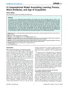
The static MAE The static MAE is induced by relatively slow adapting motion, in the region of 12-20°s-1 (van de Grind, 2003), and exhibits both spatial and temporal frequency tuning. The effect seems strongest when the spatial frequencies of the adapting and test gratings are the same (Cameron et al, 1992; Ashida and Osaka, 1994; figure 1A), but this peak strength seems to be relatively constant for a wide range of matched spatial frequencies (Wright and Johnston, 1985). Temporally, the effect seems to peak when the adapting grating has a temporal frequency of about 5-10Hz (Pantle, 1974; Wright and Johnston, 1985; Ashida and Osaka, 1995; figure 1B). The static MAE also varies with the relative contrasts of the adapting and test gratings. For a given test grating contrast, the strength of the effect increases with the contrast of the adapting grating. However, it saturates once the adapting contrast exceeds the test contrast. Conversely, for a given adapting contrast the MAE is stronger for test gratings with lower contrasts (Keck et al, 1976; Nishida et al, 1997).

1

Whether or not the static MAE exhibits speed tuning is unclear. Wohlgemuth (1911) suggested that MAE strength initially increases steeply with adapting speed before peaking and then gradually declining. Mather et al (1998) reference studies by Granit (1928) and Scott and Noland (1965) that put the peak adapting speed at 2.5°s-1 and 3°s-1 respectively. However, it is not clear if any of these experiments varied the spatial frequency of their stimuli in order to separate any velocity tuning from any temporal frequency tuning. Verstraten et al (1998) measured the static MAE induced by a random dot kinematogram (RDK). In the adapting stimulus, all the dots moved in the same direction and in the test stimulus all the dots were stationary. A random dot pattern is often known as "white noise" because it contains a wide range of spatial frequencies. Using such stimuli should therefore reveal any velocity tuning of the MAE. Verstraten et al found that the static MAE peaked at adapting velocities of 3-6°s-1 (figure 1C). This is inconsistent with the invariance of temporal frequency tuning with spatial frequency reported by Wright and Johnston (1985). However, it is consistent with the leftwards shift in peak temporal frequency with increasing adapting spatial frequency reported by Ashida and Osaka (1995). It would be interesting to see the temporal frequency tuning data re-plotted in terms of adapting velocity for comparison with the Verstraten et al velocity tuning data.

A

B

C

Figure1: A: Spatial frequency tuning of static MAE. Each curve illustrates how the strength of the MAE varies with test spatial frequency for a different adapting spatial frequency. For adapting frequencies of 0.5cpd and above, the MAE is strongest when the test and adapting frequencies match (cpd=cycles per degree). All stimuli had a temporal frequency of 5Hz (Cameron et al, 1992); B: Temporal frequency tuning of static MAE, showing the variation in MAE strength with the temporal frequency of the adapting grating. Each set of shapes is for a test grating of different spatial frequency (diamonds=2.45cpd, squares=6.13cpd, triangles=9.8cpd. Note how a single curve fits the data for all three spatial frequencies well (Wright and Johnston, 1985); C: Velocity tuning curves for the static (closed circles) and dynamic (open symbols) MAE measured by Verstraten et al (1998) using random dot patterns.

The dynamic MAE As mentioned previously, the dynamic MAE is elicited by the presentation of "dynamic" test stimuli such as random dot kinematograms (RDKs) or flickering "counterphase" gratings. One of the key differences between the dynamic and static MAEs is the fact that adaptation to second order motion produces a strong dynamic MAE but a very weak or non-existent static MAE (McCarthy, 1973; Nishida and Sato, 1995). First order motion is produced by the movement of a luminance 1 modulated pattern: the moving pattern is defined by changes in luminance. Second order motion is defined by the motion of a pattern defined by something other than luminance. Examples include the motion of patterns defined by contrast 2 modulation or by texture defined boundaries

1

Luminance is the physical amount of light emitted or reflected from a stimulus. In layman's terms it is a measure of the physical "brightness" of a stimulus. However, in the field of vision research brightness has a specific technical meaning. It refers to the subjective perception of the luminance of a stimulus, which depends on context. For example, the luminance of a piece of white paper in bright moonlight and bright sunlight differs by several orders of magnitude but the perceived brightness is very similar. 2 Contrast is a measure of the range of luminance values present in a stimulus. For a low contrast stimulus there is little difference between the "brightest" and darkest parts of the stimulus. For a high contrast stimulus there is a large difference between the "brightest" and darkest parts of the stimulus.

2

(figure 2). First and second order motion are also referred to as Fourier and non-Fourier motion respectively.

A

B

C

D

Figure 2: A: A luminance modulated grating that would produce pure first order motion; B: Contrast modulated random noise. This would produce pure second order motion; C: A contrast modulated luminance grating. If the luminance grating remained static, with only the contrast modulation moving, this would produce pure second order motion. However, if the luminance grating also moved this would produce a mixture of first and second order motion; D: A pattern with texture defined boundaries. The alternating stripes differ only in the scale of their random noise dots. This pattern would produce pure second order motion.

The tuning properties of the dynamic MAE are considerably less established than those of the static MAE. Evidence for spatial frequency tuning is mixed. von Grünau and Dube (1992) report similar tuning to the static MAE while Ashida and Osaka (1994) report a gradual increase in MAE with spatial frequency up to 4cpd. Ashida and Osaka (1995) also found that the evidence for temporal or velocity frequency tuning of the dynamic MAE is not clear. For a given adapting spatial frequency, temporal frequency tuning is similar to the static MAE. However the precise shape and positioning of the curve varied significantly with adapting spatial frequency. Velocity tuning shows similar properties. Ashida and Osaka conclude that the dynamic MAE is more likely to be tuned to velocity than temporal frequency. However, they admit that the velocity dependence is not very robust. While the studies discussed above measured the dynamic MAE using a flickering static "counterphase" grating, Curran and Benton (2006) measured it using random dot kinematograms (RDKs) as adapting and test stimuli. In the adapting stimulus all the dots moved in the same direction (100% coherence), while in the test stimulus the dots moved in random directions (0% coherence). They found that the strength of the MAE did not vary with the speed of the dots in the adaptor stimulus but did vary with the speed of dots in the test stimulus. However, these results are in disagreement with those reported by Verstraten et al (1998). Although the Verstraten et al study only explored only one test velocity, it clearly shows that MAE strength varies with adapting velocity. It should be noted that, rather than dots moving in random directions as used by Curran and Benton, the test stimulus in this case was dynamic visual noise. The former stimulus contains coherent local motion cues as each dot has a fixed direction for its translation across the stimulus field. The latter contains no local motion cues as dots randomly wink in and out of existence at each time step. This difference in test stimulus could explain the difference in observed MAE velocity tuning. Additional studies have used moving gratings as the test stimuli (Thompson, 1981; Smith, 1985; Ledgeway and Smith, 1997). In these studies the after-effect is a reduction in the perceived speed of stimuli moving in the same direction as the adaptor. This effect is sometimes known as the velocity after-effect. However it seems clear that it is strongly related to the MAE and is likely to be simply a different manifestation of the same underlying mechanisms. These studies report that the after-effect is negligible when the speed of the test stimulus is greater than that of the adaptor and then rapidly falls to a minimum as the speed of the test stimulus falls below that of the adaptor. In general it appears that the various tuning properties of the dynamic MAE are much less clearly understood than those of the static MAE. It should be noted that it is generally non-trivial to compare reported MAEs due to differences in the methods used to estimate its strength and the range of different adapting and test stimuli used.

3

Theories of the MAE It is generally agreed that the MAE arises as a result of adaptation within the visual system to the motion of the adaptor. As early as 1963 Barlow and Hill had demonstrated that directionally selective cells in the rabbit retina gradually reduced their activity during prolonged exposure to motion in their preferred direction, but experienced no such reduction in activity in response to motion in the opposite direction. Hammett et al (2000) have shown a similar reduction in perceived speed with exposure time in human psychophysical experiments. Barlow and Hill considered an opponent system of two cells selective for opposite directions of motion, with the perceived direction of motion determined from the relative activity of these two cells. Following adaptation to motion in one direction, the activity of the cell selective for the adaptation direction will be reduced below its baseline level, while the activity of the other cell will remain at its baseline level. There will therefore be a weak motion signal in the opposite direction to the adapting motion. Sutherland (1961) proposed a similar idea with a population of cells tuned for a variety of directions, where the perceived direction of motion is determined by an average of the population activity. Following adaptation to a particular direction, the activity of cells responsive to that direction would be reduced, biasing the population motion estimate in the opposite direction. It should be noted that both these theories require a baseline level of activity in order to induce the static MAE. This is supported by the physiological evidence,which indicates that cells in the retinal and visual cortex have a sustained baseline activity of approximately 10% of their maximum activity, so this is a biologically plausible assumption (Barlow and Hill, 1963; Crowder et al, 2006). Presentation of a dynamic stimulus following adaptation would excite cells tuned to a variety of directions. However, the activity of the adapted cells would remain lower than the unadapted cells and the motion bias would remain. These theories would also explain the postadaptation reduction in perceived speed of stimuli moving in the same direction as the adaptor. The consensus view is that the static and dynamic MAEs result from adaptation at different locations in the visual system. However, there is no clear agreement on where these locations are or what differentiates them from each other. Ashida and Osaka (1995) propose separate first and second order motion channels, with the static MAE caused by adaptation within the first order channel and the dynamic MAE caused by adaptation at a later stage that integrates inputs from the two channels. However van der Smagt et al (1999) propose that the static and dynamic MAEs are caused by the independent adaptation of slow and fast motion channels with different temporal tuning characteristics. There is evidence to support both these views. von Grunau and Dube (1992) found that the dynamic MAE could be seen outside of the adapting area, whereas the static MAE could not. This supports the theory that the dynamic MAE is caused by adaptation at a higher level than the static MAE, where inputs from a wider area are integrated. On the other hand, the work by van der Smagt et al with transparent patterns supports the separately adapted fast and slow channel theory. In a transparent pattern, two populations of dots move at two different velocities and both motions are simultaneously perceived. This contrasts with "plaid" patterns, where two gratings move at different velocities but are perceived as a single composite pattern ("plaid") moving in the vector average of the component velocities. van der Smagt et al used a transparent pattern containing both fast and slow components as the adapting stimulus. For low temporal frequency test stimuli the MAE was seen in the direction of the slow component, while for high frequency test stimuli the MAE was seen in the direction of the fast component. Most interestingly, when a test stimulus containing both high and low frequency components was used, both MAEs were seen transparently. Given the evidence for multiple sites of adaptation contributing to the dynamic MAE, it is perhaps unsurprising that characterisation of its tuning properties has been difficult to establish. Additional evidence for multiple sites of adaptation is provided by the phenomenon of MAE storage. The typical duration of either static or dynamic MAE is of the order of 10-15 seconds. However, if a blank stimulus is presented for this amount of time prior to the presentation of the test stimulus, the MAE is still perceived (Spigel, 1962). In fact, a surprising range of intervening

4

stimuli can be displayed in this "storage" period between adaptation and testing and still maintain the MAE (Thompson and Wright, 1994). Most interestingly, Verstraten et al (1996) experimented with alternating static and dynamic test stimuli after a single adaptation period. They found that, when the dynamic stimulus was presented first, the strength of the subsequent static MAE was relatively unaffected. However, when the static stimulus was presented first, the strength of the subsequent dynamic MAE was severely reduced. Essentially, the static MAE exhibits storage during the induction of the dynamic MAE, but the reverse does not hold, providing further evidence in support of different sites of adaptation.

Models of the MAE Various models of motion adaptation have been proposed to explain the MAE. Most of them involve changing the gain of different channels as a function of the response of the channel to the adapting stimulus. In some cases these are two directionally opponent channels (Sachtler and Zaidi, 1993; van de Grind, 2003). In others the channels differ in their temporal frequency tuning (Smith and Edgar, 1994). van Boxtel at al (2006) propose a "channel-less" approach where the change in gain varies with the adaptability of a population of neurons with a wide range of preferred speeds and orientations. However, this is conceptually very similar to the directionally opponent channel models, but extended to a population-based velocity estimate. Another approach is to vary the temporal response properties of the channels. Clifford et al (1997) change the temporal delay of an opponent motion detector as a function of its response to the adapting stimulus. These models are discussed in more detail in the Modelling Theory section.

Project aims With the notable exception of Clifford et al, most of the models described above are relatively abstract in nature and are not actual functional models of motion detection. The three standard models of biological motion detection are the correlation model (Reichardt, 1961; as implemented by Clifford et al), the gradient model (Fennema and Thompson, 1979) and the motion energy model (Adelson and Bergen, 1985). The correlation model has largely fallen out of favour for modelling mammalian vision (Emerson et al, 1992). Therefore the goal of this project was to incorporate adaptation into one or both of the gradient or energy models in order to determine to what extent adaptation in these models can explain the MAE. As the tuning properties of the static MAE are considerably more established than those of the dynamic MAE, the properties of the models will be primarily compared to the experimental data on the static MAE to evaluate how well the models explain the MAE.

5

Modelling theory Models of motion processing As mentioned in the introduction, the three standard model of motion detection are the Reichardt correlation detector (Reichardt, 1961), the gradient model (Fennema and Thompson, 1979) and the motion energy model (Adelson and Bergen, 1985). The Reichardt correlation model is now generally considered to be inconsistent with mammalian physiological data (Emerson et al, 1992), although it is still considered to be a good model of insect vision. Consequently this study will focus on the gradient and energy models. However, one of the adaptation methods considered has been implemented in the correlation model, so a brief overview of its workings will be useful.

The correlation model In this model, two luminance detectors are separated by small distance Δx (marked 1 and 2 in figure 3). The output of each of these two detectors is passed through two channels. The first channel goes directly to a correlation unit associated with each detector (marked A and B in figure 3). The second channel passes a delayed signal to the correlation unit associated with the other channel. Examining figure 3 it can be seen that a stimulus passing from left to right would activate detector 1 first before activating detector 2 a short time Δt later. At time Δt, correlation unit B will receive both the immediate signal from detector 2 and the delayed signal from detector 1. These two signals will be identical and its output will therefore be large. In contrast, the output from correlation unit A will be very small as there will be no correlation between the immediate signal from detector 1 and the delayed signal from detector 2. The outputs of the two correlation units are then differenced, with the output of unit B subtracted from the Figure 3: A Reichardt correlationoutput of unit A. In this case this will produce a negative motion cased motion detector signal, signifying rightwards motion. Conversely, for motion to the left, the signal from A will be high and the signal from B will be low. This will result in a positive motion signal, signifying leftwards motion.

The gradient model The first clear description of the gradient model was by Fennema and Thompson (1979), building on earlier work by Limb and Murphy (1974). A more formal treatment of the model is given in Johnston et al (1992) and is expanded upon here. Consider a 1D pattern with intensity defined by the function I(p), where p is the distance from the origin within the pattern. If this pattern is moving in 1D space, the intensity of the pattern can also be described by the function I(x,t), where x and t define the position in a 2D space-time. The space-time surface I(x,t) can be constructed by translating the 1D pattern I(p) in space and time, forming a 2D surface with oriented isoluminance contours (figure 4). Each point p will trace a contour of constant luminance in space-time with a gradient equal to the velocity of motion at that point. As time monotonically increases along each of these contours, this "conservation of luminance" property can be formalised by constraining the temporal derivative of I(x,t) to be zero along all of these contours (equation 1A). Expanding this full derivative in terms of partial derivatives in x and t (equation 1B) gives an estimate for the velocity of motion (equation 1C).

6

Conservation of luminance

dI ∂I dx ∂I ∂I ∂I = + = v+ = 0 [Eq. 1B] dt ∂x dt ∂t ∂x ∂t

dI = 0 [Eq. 1A] dt v=−

∂ I ∂t [Eq. 1C] ∂I ∂x

Pattern constancy ∂I d ⎛ ∂I ⎞ = c ⇒ ⎜ ⎟ = 0 [Eq. 2A] ∂x dt ⎝ ∂x ⎠ d ⎛ ∂I ⎞ ∂ ⎛ ∂I ⎞ ∂ ⎛ ∂I ⎞ ∂ 2 I ∂2I = 0 [Eq. 2B] ⎜ ⎟ = ⎜ ⎟v + ⎜ ⎟ = 2 v + dt ⎝ ∂x ⎠ ∂x ⎝ ∂x ⎠ ∂t ⎝ ∂x ⎠ ∂x ∂t∂x Figure 4: Bottom: A 1D pattern defined by

the function I(p); Top: This pattern moving in 1D space can be represented by the 2D space-time surface I(x,t). Each point p in the 1D pattern traces an isoluminance contour in space-time.

v=−

∂ 2 I ∂t∂x 2

∂ I ∂x

2

[Eq. 2C]

v=−

∂ n +1 I ∂t∂x n −1 ∂ n +1 I ∂x n

{n ≥ 2

[Eq. 2D]

It can be seen that for motion in 1D the velocity is simply the ratio of the partial temporal and spatial derivatives of the space-time image. This ratio is undefined when the partial spatial derivative is zero, making this velocity estimate ill-behaved at peaks and troughs in the 2D spacetime luminance surface I(x,t). However, along each of the isoluminance contours traced in spacetime by the points of the 1D pattern I(p), the pattern in the x direction either side of the contour remains constant. This "pattern constancy" can be formalised by constraining the spatial partial derivative of I(x,t) to be constant along any of these contours. This is equivalent to constraining the temporal derivative of this partial spatial derivative to be zero along these contours (equation 2A). Expanding this full derivative in terms of partial derivatives in x and t (equation 2B) gives a second estimate for the velocity of motion (equation 2C). In fact, as the pattern around each contour is constant in the x direction, all the higher orders of partial spatial derivatives will also be constant along isoluminance contours. Therefore any number of velocity estimates may be constructed in the same manner as the one above to give a family of estimates conforming to equation 2D. Note that for 1D motion the estimate derived from conservation of luminance fits nicely into this family as the special case where n=1. Clearly each of these estimates is undefined when the relevant order partial spatial derivative is zero. However, the partial spatial derivatives for all orders are unlikely to be zero at the same time. Therefore a combination of these estimates should provide a robust velocity estimate at all points in spacetime. The only situation in which all the orders of partial spatial derivative will be the zero is when the 1D pattern has no spatial structure around the point p. This means that a gradient model will not provide a good estimate of velocity for points in an image where there is a lack of spatial variation over a region larger than that over which the model computes its various order derivatives. This will be referred to as the "uniformity problem". For motion of 2D patterns in 3D space-time, two partial derivative equations are required for each velocity estimate, as both the horizontal and vertical components of velocity are unknown in each equation. In this case conservation of luminance is insufficient as it only provides a single equation regardless of the number of spatial dimensions. One option would be to assume that the luminance gradient is conserved. However, this assumes that the pattern is moving at a constant velocity over time, which may not be the case. A better option is to extend the estimates derived from pattern constancy. For a moving 2D stimulus the pattern around space-time isoluminance contours is conserved in both x and y directions. This provides two equations for each order of

7

partial spatial derivative that can be combined to produce estimates for the horizontal and vertical components of velocity. As with 1D motion, 2D motion also suffers from the "uniformity problem". All velocity estimates are ill-conditioned when there is a lack of spatial structure over a region larger than that over which the model computes its various order derivatives. However, there is an additional issue when considering motion of a 2D pattern. The velocity estimates are also illconditioned where the pattern is inherently 1D (i.e. varies only in the horizontal or vertical directions). In this case all orders of partial spatial derivative orthogonal to the direction of variation will be zero and this component of the velocity estimate will be undefined. This means that there will be a continuum of horizontal and vertical component velocities that are compatible with the resultant space-time pattern. This is known as the "aperture problem" and can be considered a special case of the "uniformity problem" where the lack of variation exists along only one of the space dimensions. For this study, the gradient model implementation was based on that of Johnston et al (1992). This model uses Gaussian derivatives for the various derivative filters. Filtering the space-time image with these filters is equivalent to calculating the various order partial derivatives of the space-time image blurred with a Gaussian filter. The detail of the implementation is covered in the next section. Although the Gaussian derivative filters of the gradient model are designed to calculate various orders of partial derivatives, their receptive fields closely resemble the fields of some of the simple cells found in the primary visual cortex (figure 5).

Figure 5: Top: Space-time plots of selected Gaussian derivative filters as used in the Johnston et al (1992) gradient model implementation; Bottom: Selected 2D spatiotemporal receptive fields of simple cells in macaque monkey primary visual cortex. [Source: DeValois et al (2000)]

The energy model The reference paper for the energy model is Adelson and Bergen (1985). This describes the use of a system of oriented space-time filters to compute the "motion energy" of a stimulus, building on previous work by Burr and Ross (1983) and Watson and Ahumada (1983). The energy model also considers 1D motion as a pattern in 2D space-time, with the orientation of this pattern dependent on the velocity of the stimulus. This orientation can be determined using detectors that are oriented in space-time, thus providing a measure of the stimulus velocity (figure 6A-C). However, while such oriented space-time filters are selective for motion at particular velocities, their response generally varies with both the position of the filter in space-time and the contrast of the stimulus. Consider the filter in figure 6C-E. Positioned at the right hand edge of the low luminance stripe (C), the filter's positive region is entirely covered by high luminance areas of the stimulus and its negative region is covered entirely by low luminance areas. Consequently the filter's response is highly positive, as expected for this stimulus, which is at the filter's preferred

8

orientation. However, if the filter is displaced to the left so that it straddles the right edge of the low luminance stripe (D) its positive region is now covered entirely by low luminance areas of the stimulus and its negative region by high luminance areas. As a result its response is highly negative. Similarly, if the filter remained at the left edge of the stimulus strip but the stimulus was changed to a high luminance bar moving on a low luminance background (E) the filter's response would also be negative. Filters with outputs which vary in this manner are considered "phase dependent".

A

B C

D v = vpref

v = vpref

E v = vpref

Figure 6: A: Velocity can be considered to be equivalent of orientation in space-time. For example a bar moving in the x direction will produce an oriented trace in the x-t plane; B: The orientation of this trace will depend on the speed of the bar in the xdirection; C: The orientation of this trace can be detected by a population of filters that are orientated in the x-t plane. However the filter's response is not constant with position in space-time (D) or stimulus contrast (E). [Source: Adapted from Adelson and Bergen (1985)]

Adelson and Bergen proposed a solution to the phase dependence problem based on summing the squared output of two detectors which are 90° out of phase in space-time (figure 7A). Such are pairs of detectors are "in quadrature" with one another and the sum of their squared outputs is known as "motion energy". This is most easily understood by considering the "ideal" case where the filters are 2D Gabor functions oriented in space-time. A Gabor function is any sinusoidal function modulated by a Gaussian envelope. In this case it is convenient to select the sine and cosine functions to obtain a quadrature pair, but any sinusoids out of phase by 90° would work equally well. In this special case, the cosine-based Gabor is known as the "even" filter and the sine-based Gabor is known as the "odd" filter (figure 7B-C). Using the relation cos2(θ) + sin2(θ) = 1, it is clear that summing the squared outputs of such a quadrature pair of Gabor filters will produce a phase-independent response. The square root of this motion energy response is often used as the energy model output to match the scale of the quadrature pair outputs. Gabor functions have some properties that make them particularly convenient filters for motion energy models. The functions were developed by Gabor (1946) as the optimal functions for providing a description of a signal that is well localised in both the space-time and frequency domains. In other words, Gabor functions are the theoretically optimal functions for simultaneously localising a stimulus in space-time and characterising its spatial and temporal frequency composition. Gabor functions are especially attractive as velocity tuned filters as the frequency representation of a 2D Gabor is two Gaussians situated at radial distances +/- r on a line through the origin in frequency space (figure 7D). The orientation of the line is determined by the orientation of the sinusoidal variation of the filter, and is thus rotated 90° counter-clockwise from the spatiotemporal orientation of the filter. The distance r is determined by the frequency of the sinusoid component of the filter. Thus a Gabor filter is an ideal filter for detecting the motion of spatial structure at a preferred velocity (set by the orientation of the filter) and spatiotemporal scale (set by the frequency of the filter's sinusoid). However the spatiotemporal scale r is a fixed polar distance from the origin in frequency space. Therefore the projection of r onto the spatial and temporal frequency axes will vary depending on the orientation of the filter. As a result filters tuned to different velocities will have different preferred spatial and temporal frequencies. Additionally, if the filter's Gaussian envelope is not circularly symmetric, the width of this spatial and temporal tuning will also change with the filter's velocity tuning.

9

A

B

C

D

Figure 7: A: The computation of motion energy by summing the squared output of a quadrature pair of linear filters [Source: Adelson and Bergen, 1985]; B: 1D even (top) and odd (bottom) Gabor functions. The Gabor functions are shown in solid blue and the modulating Gaussian envelopes in dashed red; C: 2D oriented even (top) and odd (bottom) Gabor filters. Red areas indicate high positive weightings. Blue areas indicate high negative weightings; D: The magnitude of the spatiotemporal frequency representation of the even (top) and odd (bottom) 2D Gabor filters in C. Note that the frequency representations of the two

filters differ only in phase and therefore their magnitudes are identical. The frequency representation of a Gabor filter is a pair of Gaussians situated at radial distances of +/- r on a line through the origin. The orientation of the line is determined by the orientation of the sinusoidal variation of the filter; the distance r is determined by the frequency of the sinusoid; and the width of the Gaussians is inversely proportional to the width of the filter's Gaussian envelope. If the filter has an elongated Gaussian envelope, then the Gaussians in frequency space will also be elongated, but in a perpendicular direction. Although Gabor filters have some nice theoretical properties, they are not necessarily biologically plausible. Figure 8 shows some experimentally measured spatial (cat; Jones and Palmer, 1987; AB) and spatiotemporal (macaque; De Valois et al, 2000; C-H) receptive fields in primary visual cortex 3 . While many can be reasonably approximated by a Gabor function, the regions of these receptive fields generally do not have a well defined width. Different regions are often different widths and the same region often varies in width along its length in a manner inconsistent with a Gabor function. Additionally, the side lobes of the receptive fields are often skewed relative to the major axis, again inconsistent with a Gabor function. Other studies have found similar results (Burr et al, 1986; DeAngelis et al, 1985). It might be argued that these deviations from the "ideal" Gabor filter are simply the result of biological "noise" in the development of the receptive fields. However, DeValois et al (2000) performed principle component analysis (PCA) on the oriented fields they measured and found that they could be considered to be the sum of two linearly separable non-oriented fields. These component fields bear a striking resemblance to two of the non-oriented receptive fields measured in the same study (compare figure 8 I and J to D and E). Interestingly the generation of oriented receptive fields by the summing and differencing of nonoriented linearly separable fields was suggested by Adelson and Bergen in their original 1985 paper.

3

V1 in primates; area 17 in cats and other mammals.

10

A

F

B

G

C

D

E

H

I

J

Figure 8: A,B: 2D spatial receptive fields of simple cells in cat primary visual cortex as measured by Jones and Palmer (1987). A: A spatially separable receptive field that could be well modelled by a Gabor function; B: A spatially inseparable receptive field that might be reasonably modelled by a Gabor function but has significantly skewed lobes; C-H: 2D spatiotemporal receptive fields of simple cells in macaque monkey primary visual cortex as measured by De Valois et al (2000). C,F: Two linearly separable receptive fields that might be reasonably modelled by a Gabor function but have significant variation in lobe width; D: A linearly separable receptive field that would be well modelled by a Gabor function; E,G: Linearly separable receptive fields that could not be modelled by Gabor functions; H: An oriented non-separable receptive field that might be reasonably modelled by a Gabor function. However, it is interesting to note that its principle components (I and J) are very similar to the receptive fields in D and E. This suggests that oriented V1 cells might be constructed by summing and differencing the responses of linearly separable, non-oriented neurons earlier in the V1 pathway. Note that C,D,E,G are the same plots as shown in figure 5. They are repeated here for ease of reference. [Source: A,B: Jones and Palmer, 1987; C-J: De Valois et al, 2000]

Indeed, many implementations of the energy model have not used Gabor filters (Wilson et al, 1992; Simoncelli and Heeger, 1998), or have limited them to defining the spatial receptive fields, opting for more biologically plausible temporal responses (Watson and Ahumada, 1983; Klam et al, 2008). Interestingly, some models use the same Gaussian derivative based filters that are used in the Johnston et al gradient model. However, despite the fact that more biologically plausible filters exist, Gabor filters remain a reasonable approximation for modelling such fields and other energy model implementations have used Gabor filters oriented in both space and time (Heeger, 1987; Baker, 2001). For the purposes of this study Gabor filters were selected primarily for their well-defined frequency response. It was felt that this would provide the "cleanest" background against which to observe the effects of adaptation on the output of the model. The detail of the implementation is covered in the next section.

Models of adaptation As mentioned in the introduction, most models of motion adaptation adapt the gain of different channels as a function of the response of each channel to the adapting stimulus. Some differentially adapt two opponent directionally selective channels (Sachtler and Zaidi, 1993; van de Grind et al, 2003), while others differentially adapt two channels with different temporal frequency tuning (Smith and Edgar, 1994). The other interesting approach is that of adapting the temporal delay characteristics of the motion detectors in a model. Clifford et al (1997) implemented this in a correlation-based Reichardt detector model. However, the concept can be applied very easily to the gradient model and with some effort could be approximately implemented in the energy model. In fact Langley (2000) incorporated a variant of this adaptation method into an

11

energy/gradient hybrid model based on Gabor derivatives and principle component analysis. Finally, consideration is given to the adaptation of sigmoidal transfer functions. The response of neurons in many levels of the visual system vary in a characteristic manner as the contrast of a stimulus is varied (figure 10). The shape of this "contrast response" function is thought to reflect the fact that the firing rate of a neuron is constrained to be positive and has a limited range. Conceptually it can be considered to place "soft" upper and lower limits on the firing rate of the neuron. Visual neurons are often modelled as performing linear summations on their inputs, and passing the linear output of a neuron through a sigmoidal "transfer" function is a common method of constraining it to a biologically plausible range. From an adaptation perspective, such transfer functions are interesting as motion adaptation has been shown to change the properties of the contrast response functions of neurons in the visual system.

Adapting the gain of directionally selective channels Both Sachtler and Zaidi (1993) and van de Grind et al (2003) propose models in which the gains of two opponent channels selective for leftwards and rightwards motion are independently modified as a function of their responses to the adapting stimulus. In both models each channel's pre-gain response to a test stimulus is denoted as xT, and this is transformed into its post-gain response RT via multiplication with a gain factor g (equation 3A). In both cases the adaptive change in gain is non-linearly dependent on the response of the channel to the adapting stimulus, denoted as xA, and the maximum gain is 1 when the channel has no response to the adaptor. However, at first glance the form of the relationship linking g and xA appears to differ significantly between the models (equations 3B and 4A).

RT = g.xT [Eqn 3A]

g=

1 [Eqn 4A] 1 + w.x A

g=

k k + (x A ) p

g min =

[Eqn 3B]

g min =

k k + (x max ) p

⇒k=

g min (x max ) p [Eqn 3C] (1 − g min )

(1 − g min ) [Eqn 4B] 1 ⇒w= g min x max 1 + w.x max

Upon close inspection however, it can be seen that the two models are equivalent. Consider the problem of setting the parameters of each model to obtain a desired minimum gain gmin. This minimum gain will occur when the channel responds maximally to the adapting stimulus (i.e. xA = xmax). Equations 3C and 4B derive expressions for gmin in both models, in terms of this maximum response xmax and the model parameters. It is immediately clear that the parameters k, p of the Sachtler and Zaidi model can be translated into an equivalent parameter w in the van de Grind et al model (equation 5). Note that Sachtler and Zaidi set p to 1 in their model, so this simplifies further into a straightforward reciprocal relationship between k and w. w=

(x max ) p −1 k

⇒w=

1 {p = 1 [Eqn 5] k

It would be simple to implement this type of adaptation for the energy model by adapting the response of each oriented motion energy filter as per equation 3 or 4. In principle it should be possible to do exactly the same with the various partial derivative filters in the gradient model. However, adapting the gain of the gradient model filters will not have the desired effect for any velocity estimates based simply on the ratio of two filter responses. The obvious case is when the velocity of the adaptor is 1. For any velocity estimate that is simply the ratio of two filter responses, both sets of responses will be equal. Therefore both filters will be adapted to the same extent and their post-adaptation responses to a stimulus of any velocity will remain unchanged. The experimental evidence for the MAE doesn't support this. However, the composite estimate combines filters that have different responses at a velocity of 1 and these will be adapted to different extents. Therefore this adaptation method might be applicable to the gradient model if the composite velocity estimate is used.

12

While this method of adaptation might result in a reduction of post-adaptation velocity estimates in the gradient model, it will certainly not produce the static MAE. Changing such a multiplicative gain can never change the sign of the filter's response and thus all adapted velocity estimates will be the same sign as the unadapted velocity estimates. It could be argued that neurons do not have negative responses and that the gradient model is therefore biologically implausible. The question is then how to change the model in a manner that restricts its filters to positive outputs but retains its essential character. One option might be to add an inverted copy of each filter to the model and make these filters inhibitory. However, this simply splits the standard filter response into positive and negative channels before recombining at the division stage and is equivalent to permitting the filters to have negative responses. Adapting the separate channels based on their response to the adaptor would have the same effect as adapting the original combined filter. Therefore nothing is gained by this approach and a more substantial change to the model would be needed.

Adapting the gain of channels tuned for temporal frequency Smith and Edgar (1994) propose a model of motion adaptation where the sensitivities of two broadly tuned temporal filters are independently adapted based on their individual sensitivity to the adapting motion (figure 9). One filter (L) is low-pass, most sensitive to stimuli of a low temporal frequency. This filter will also respond strongly to non-flickering static stimuli. The other filter (B) is band-pass, most sensitive to higher temporal frequencies. The proposed filters are similar to those observed in psychophysical studies (Hess and Snowden, 1992), so such a model is biologically plausible. If the adapting stimulus has a high temporal frequency, filter B will be suppressed to a greater extent than filter L, resulting in an underestimation of the temporal frequency (and thus speed) of subsequent test stimuli, as observed in the MAE (figure 9A). However the model also predicts an overestimation of speed when the adapting stimulus has low temporal frequency, as filter L will be suppressed more than filter B (figure 9B). Smith and Edgar claim that this is not observed experimentally and propose that B might be substantially more susceptible to adaptation than L, which has some support in the experimental literature (Hammett et al, 1994). Given a sufficient difference in susceptibility, this could ensure that filter L is never suppressed more than filter B. However, Ledgeway et al (1997) found that adaptation to low temporal frequency stimuli does result in an overestimation of speed when probed with a high frequency test stimulus. This is not inconsistent with the Hammett et al findings as the test stimuli used in that study were always the same frequency as the adapting stimuli. Therefore the study never tested low frequency adaptation with a high frequency test stimulus. Therefore, the experimental evidence may not be inconsistent with equally adaptable channels. The model also predicts that adaptation to a stationary counterphase grating flickering at a high temporal frequency would also produce a static MAE. It is not clear whether this has been tested experimentally. Smith and Edgar propose two alternative methods of calculating the appropriate sensitivity reduction, a multiplicative method and a subtractive method (equation 6).While Smith and Edgar found that subtractive adaptation gave the best fit between their model and the data, their model was relatively abstract. Therefore either method might be a candidate for incorporating adaptation in the gradient or energy models. The temporal filters in the gradient model are similar in form to those employed by Smith and Edgar. Given that convolution and scalar multiplication are associative, adaptive rescaling of the gradient model temporal filters could be achieved by rescaling the response of the temporal filters to the test stimulus based on the response of each filter to the adapting stimulus. Either adaptation method could be incorporated into the energy model by rescaling the response of each filter to the test stimulus based on its response to the adapting stimulus. However, as the Gabor filters are not separable, it would not be possible to adapt the filters based purely on their temporal sensitivity.

13

A

B

Figure 9: Motion adaptation in Smith and Edgar (1994) is achieved by adapting the sensitivity of two broadly tuned temporal filters based on their sensitivity to the adapting stimulus - a low pass filter (L) and a band pass filter (B). A: When the

adapting stimulus is of high temporal frequency, B is suppressed more than L and the perceived temporal frequency (and thus speed) of subsequent stimuli will be reduced. This corresponds with the observed MAE; B: However, when the adapting stimulus is of low temporal frequency, L will be suppressed more than B and the perceived temporal frequency (and thus speed) of subsequent stimuli will be increased. [Source: Smith and Edgar (1994)] Multiplicative ⎛ S ⎞ F * = F ⎜1 − k a ⎟{0 < k < 1 ⎜ S p ⎟⎠ ⎝

[Eqn 6A]

Subtractive F* = F − k

Sa {k > 0 Sp

Equation 6: Two alternative adaptation methods from Smith and Edgar (1994) A: Multiplicative adaptation; B: Subtractive adaptation. In both cases F* is the adapted filter function; F is the unadapted filter function; k is a constant determining the strength of adaptation; Sa is the sensitivity of the filter to the adapting stimulus; Sp is the peak sensitivity of the filter.

[Eqn 6B]

Adaptation of temporal delay Clifford et al (1997) present a model of motion adaptation based on the Reichardt correlation detectors described above. The temporal delay filters in the standard Reichardt model are replaced by first order low-pass filters in order to permit non steady state adaptation to be modelled. Additionally the differencing of the correlation units is made unbalanced so that there is a small signal for no motion. This permits the detector to be activated by flickering stimuli. The motion signal output of the detector is fed back to the two temporal filters, with a greater motion signal resulting in a larger decrease in the time constants, reducing the effective delay between the signals from the two luminance detectors at each correlation unit. In the absence of a motion signal the time constants of the temporal filters gradually revert to their unadapted value. This type of adaptation would be very easy to implement in the Gaussian derivative based gradient model. The temporal filters in this model are derivatives of a log-Gaussian, which has two associated parameters. α sets the position of the peak response and τ sets the decay constant for the tail. Either or both of these parameters could be reduced to decrease the effective delay of the temporal filters. However, a reduction in α is likely to have the greatest effect. The question is what signal to use to drive the adaptation. Although the Clifford et al model uses the overall motion signal of the Reichardt detector to drive adaptation, each Reichardt detector effectively only has one temporal delay filter (both filters are identical intoning and are adapted in unison). However, the gradient model has three differently tuned temporal filters. Given the observed properties of the MAE, it seems most appropriate to use the response of each temporal filter to the adapting stimulus to drive the reduction of its temporal delay. Langley (2000) uses a somewhat more complex feedback mechanism, and this could also be explored. It has the advantage of being prior art of gradient model adaptation via the adjustment of its temporal filters. However the adaptation method is substantially more complex, requiring 6 parameters and recursive feedback. In spite of the model's complexity its output gives a rather ambivalent fit to the data. An

14

approach based on direct manipulation of the temporal filter parameters is preferred as it is more straightforward both to theoretically analyse and relate to the properties of neurons in the visual cortex. Implementation of such an adaptation method in the energy model suffers the same problem as adjusting the gain of the temporal filters. The Gabor-based filters are inseparable and it is therefore not possible to adjust the temporal delay in isolation. Additionally, filters tuned for different orientations in space-time will have different delays. However, it is possible to imagine a heuristic that would adjust the temporal frequency properties of each Gabor filter in proportion to its response. However, this would likely result in a very inhomogeneous population of filters and would still result in some inevitable changes to the spatial tuning of each filter. For this type of adaptation it might be more appropriate to use filters that have an independently adaptable temporal response. Using oriented filters constructed from the sums and differences of linearly separable filters would permit the temporal delays of these component filters to be adapted independently of their spatial frequency tuning. This is discussed further in the Modelling Implementation section.

Adapting transfer functions The relationship between the contrast of a stimulus and the corresponding activity of a neuron is often plotted as a contrast response function (figure 10). For neurons in both visual cortex and MT this contrast response function has been experimentally determined to be well-fitted by a sigmoidal function known as the Naka-Rushton equation (Sclar et al, 1989; Kohn and Movshon, 2003; Crowder et al, 2006; equation 7). Neurons in the pre-cortical visual pathway have also been shown to have similar contrast response functions (Solomon et al, 2004). Neither the energy model nor gradient model filters exhibit such sigmoidal contrast responses in their standard form. The filter outputs vary linearly with contrast in both models. Either model could be amended to exhibit a sigmoidal contrast response by passing their "standard" responses through a sigmoidal transfer function, with the original responses taking the place of contrast in equation 7. Although this may seem an arbitrary addition to the models it does make the output of the filters more closely resemble the output of neurons which have similar receptive fields.

R = R max

c

n

n c n + c 50

+m

Equation 7: R is the current response of the neuron; Rmax is the maximum response of the neuron (above baseline); m is the baseline activity of the neuron; c is the contrast of the current stimulus; c50 is the "contrast gain", which is the contrast for which the activity of the neuron is at half maximum (above baseline); n is a scaling power that determines the steepness of the contrast response function.

Kohn and Movshon investigated how this contrast response function varied for MT neurons after adaptation to drifting gratings. They found that for some neurons adaptation was best modelled by a reduction in Rmax, while for other it was best modelled by an increase in c50. A reduction in Rmax is equivalent to changing the multiplicative gain in either the van de Grind or Smith and Edgar adaptation models, and either of these models could be used to determine a suitable postadaptation value for Rmax. However, changing c50 has no parallel in the previous adaptation methods. It has been suggested that such a mechanism permits the neuron to adapt its response to keep the steepest portion of its response curve close to the average properties of the scene. This would ensure that the largest changes in response occurred for variations around the current mean and serve to maximise discrimination for such variations. Generalising to the filters in our energy and gradient models, it is immediately clear that increasing c50 will results in lower activation compared to the unadapted response and thus should have the same direction of effect as a reduction in multiplicative gain. However, how these two adaptation methods vary with the properties of the adapting and test stimuli may well be different.

15

A

B

C

Figure 10: A: A sketch of the effects of varying the parameters of the Naka-Rushton equation on a neuron's contrast response function. Increasing c50 (filled black dots) results in a shift of the curve to the right, leaving the shape intact. Reducing Rmax (dotted line) compresses the curve vertically. B and C: Contrast response function for two sample neurons before (open circles) and after (filled circles) adaptation to a moving grating. For the neuron in B adaptation results primarily in a reduction in Rmax. For the neuron in C adaptation results primarily in a shift in c50.

16

Model implementation Gradient model Filter selection The gradient model used for this study is a modified implementation of the multi-channel gradient model described by Johnston et al (1992) and Johnston and Clifford (1995). The model uses a filter bank that comprises various order spatial and temporal partial derivatives of a zero order filter that is Gaussian in space and log-Gaussian in time (equation 9). Filtering the stimulus spacetime image with this filter bank is formally equivalent to calculating the various order partial derivatives of the image after it has been blurred by filtering with the zero-order filter. This can be shown by considering that filtering calculates the cross-correlation ( ⊗ ) between the image and the filter, which is equivalent to the convolution ( ∗ ) of the image with the reversed filter (equation 8A). Any order partial derivative of this convolution is equivalent to the convolution of the image with the same order partial derivative of the filter (equation 8B). Thus the cross-correlation between the image and any order partial derivative of the zero-order filter is equivalent to the same order partial derivative of the image filtered with the zero-order filter (equation 8C). r s r r r s r r r ∂ nm Fx 0 t 0 ∂ nm r r ∂n r s r ∂nF = n m I ⊗ Fx0 t 0 [Eqn 8C] I ⊗ F = I ∗ F [Eqn 8A]; r n I ∗ F = I ∗ r n [Eqn 8B]; I ⊗ Fx n t m = I ⊗ n m ∂x t ∂x t ∂x ∂x

(

i

(

)

)

i

The zero-order filter used for this implementation is the same as that described by Johnston and Clifford (1995) and uses the same parameters (equation 9). Johnston and Clifford fitted the temporal components of their filters to the psychophysical data of Hess and Snowden (1992) and this implementation uses the value of τ as adjusted to fit this data.

Fx 0 t 0 ( x, t ) =

⎛ x2 exp⎜ − ⎜ 4σ 4πσ ⎝ 1

⎡⎛ ln (τ α ) ⎞ 2 ⎤ ⎞ 1 ⎟. ⎢⎜ exp ⎟ ⎥ ; σ = 1.5;α = 10;τ = 0.268 [Eqn 9] ⎟ ατ π exp(τ 2 4) ⎢⎣⎝ τ ⎠ ⎥⎦ ⎠

For simplicity, this implementation did not incorporate the Taylor expansion local averaging stage (Johnston et al, 1992) and was limited to 2 orders of spatial derivatives rather than 8 (Clifford and Johnston, 1995). Note that, although the 1992 model did not include filters that were pure first order spatial or temporal derivatives ( Fx1t0 and Fx0t1 ), the 1995 paper introduced these and they are therefore included in this implementation. The spatial and temporal components of each filter in the model are separable. Therefore the 2D filtering operation is split into two separate 1D filtering operations for computational efficiency. The full set of discrete 1D filters included in this implementation is shown in figure 11, in both their space-time and spatiotemporal frequency representations. Note that the spatial and temporal components of the zero-order filter defined in equation 9 are normalised so that the composite space-time filter and the separated spatial and temporal filters (x0 and t0 below) integrate to 1 and that all order partial derivative integrate to zero. Therefore the lengths of the discrete 1D filters were set large enough that the first order filters summed to 1 and the higher order filters summed to less than 10-5. This resulted in filter lengths of 17 pixels for the spatial filters and 28 pixels for the temporal filters.

17

A

B

Figure 11: A: Space-time representation of the filters used in the gradient model implementation for this study; B: Spatiotemporal frequency representation of the same filters.

Velocity estimation The velocity estimate used in this implementation is a composite estimate after Johnston et al (1992). This estimate combines the "conservation of luminance" and "pattern constancy" estimates introduced in the "Modelling Theory" section above. The following derivation of this composite estimate is expanded from Johnston et al (1992). r r Consider the vectors x and t as defined in equation 10. For these vectors every pair of elements

xi and ti are linked by the equation v.xi + ti = 0 , either from "conservation of luminance" or "pattern r r constancy". Substituting v ′ = − v gives v ′xi − t i = 0 . v ′x and t can be considered to be two points in r an n-dimensional space, where the ith dimension has the same units as the ith element of t . The r scalar v′ has dimensions of x/t and converts the elements of the x vector to the same units as the r corresponding elements of t . Figure 12 illustrates this for the case where i=2. v′ can be varied to r r r produce a continuum of points v ′x , all lying on the same line. || v′x − t || is the magnitude of the r r r r distance between v ′x and t . Minimising || v′x − t || minimises the combined error of the component estimates under the constraint that they are all the same. The value of v′ which minimises r r || v′x − t || is therefore the best approximation to the true velocity. It is clear from figure 12 that this r r r distance is minimised when v′x − t is perpendicular to x . Therefore v′ best approximates −v when r r r (v ′x − t ).x = 0 . Re-arranging this condition results in the composite velocity estimate defined in equation 11.

18

r

r

Figure 12: v ′x and t plotted for the case where n=2. It can be seen that the

r r r r r distance || v′x − t || is minimised when v′x − t is perpendicular to x

r ⎛ ∂I ∂nI x = ⎜ ,..., ⎜ ∂x ∂x n ⎝

(

n ⎞ r ⎛ ∂I ⎞ ⎟ ; t = ⎜ ,..., ∂ I ⎟ [Eqn. 10] n −1 ⎟ ⎟ ⎜ ∂t ∂x ∂t ⎠ ⎠ ⎝

)

(

)

rr r r rr r r v ′ = x.t x.x ⇒ v ≈ − x.t x.x [Eqn. 11]

r r The above derivation limited the vector x to pure spatial derivatives and t to mixed derivatives r with a temporal order of 1. However x can contain any mixed derivative, so long as the r corresponding element in t is of one less spatial order and one greater temporal order. The r r composite estimate used in this study sets x and t as described in equation 12 below. r ⎛ ∂I ∂ 2 I ∂ 2 I ∂ 3 I ⎞⎟ ; , , x=⎜ , ⎜ ∂x ∂x 2 ∂x∂t ∂x 2 ∂t ⎟ ⎝ ⎠

r ⎛ ∂I ∂ 2 I ∂ 2 I ∂ 3 I t =⎜ , , , ⎜ ∂t ∂x∂t ∂t 2 ∂x∂t 2 ⎝

⎞ ⎟ [Eqn. 12] ⎟ ⎠

Filter construction The mixed partial derivatives required for the velocity estimate are calculated by filtering the 2D space-time stimulus image with a bank of 2D spatiotemporal filters constructed by combining the appropriate order 1D filters in figure 11. The full set of seven 2D filters and their theoretical frequency responses are shown in figure 13. The theoretical frequency responses were calculated by taking the Discrete Fourier Transform of each filter padded with zeros to 4 times its size to generate a high resolution frequency response plot. This theoretically calculated frequency response should match the empirical response of the filter, as the response of a finite filter to stimulus components outside its area of support is clearly zero. These theoretical frequency responses were confirmed by experimentally probing the filters with a range of stimuli of varied spatial and temporal frequencies. As the response of the filters varies with its location over the stimulus space-time image, the response of each filter was averaged over a space-time region measuring 100x100 pixels. These experimentally derived empirical frequency responses are shown for comparison. It can be seen that they are a close match to the theoretical filters. Conversion from pixel space to real world units is made via the conversion factors determined by Johnston and Clifford (1995). These are 128px per second and 111px per degree. These factors were determined by equating the theoretical 4 upper spatial and temporal frequency resolution of the full 2 temporal, 8 spatial derivative model to the 60Hz and 60 cyc/deg limits observed for humans.

4

This is the point at which the frequency response curve of the highest order temporal or spatial derivative crosses the x-axis.

19

A

∂I/∂x (x1t0)

∂2I/∂x2 (x2t0)

∂2I/∂x∂t (x1t1) ∂3I/∂x2∂t (x2t1) ∂I/∂t (x0t1)

∂2I/∂t2 (x0t2)

∂3I/∂x∂t2 (x1t2)

B

C

Figure 13: A: 2D spatiotemporal filters used in the model. Space is the horizontal axis and time is the vertical axis. The

filters have been truncated to the region centred on x=[-10..10], t=[0..20] pixels for clarity. This corresponds to a physical size of approximately 0.2 degrees by 0.15 seconds B: Theoretical frequency response of the filters as represented by their Discrete Fourier Transforms. C: Experimentally measured frequency response of the filters. In B and C spatial frequency (fx) is on the horizontal axis and temporal frequency (ft) is on the vertical axis. The responses have been truncated to the region centred on fx,ft=[-0.35..0.35] px-1 for clarity. This corresponds to a physical range of ±0.4 deg-1 by ±0.5 sec-1. Filters and their frequency response plots have been normalised to their maximum absolute value. For filter space-time plots in A red is positive, blue is negative and green is zero. For filter frequency response plots in B and C red is positive and blue is zero. The parameters of the temporal filters for the Johnston et al. gradient model have been fitted to psychophysical data from Hess & Snowden (1992). Figure 14A compares the empirical frequency response of the model to the Hess & Snowden data (the theoretical model responses are essentially identical). The Hess and Snowden data was collected using stimuli of very low temporal frequency (generally 0-1 cyc/deg). Therefore the model data used for comparison represents slices through the frequency response at approximately 1 cyc/deg. As previously reported by Johnston and Clifford (1995), there is a good fit to the data for the two band-pass filters (solid red and green), and a reasonable fit for the low-pass filter (solid blue). However, when the response curves are normalised on a common scale, it can be seen that the model's first order response (dotted red) is significantly stronger than its second order response (dotted green), and its zeroorder response (dotted blue) is very low. In fact there is no zero-order response at all for spatial frequencies of exactly zero. This can be understood by considering the range of frequency space covered by the 7 spatiotemporal filters. This is illustrated for the empirical model frequency response in figures 14B. It can be clearly seen that there is a "hole" in the model's coverage for low spatial and temporal frequencies. The zero-order response grows as the spatial frequency of the probe is increased; matches the first-order response by 5cpd; and increasingly dominates the response above this.

20

A

B

Figure 14: A: Comparison of model temporal frequency filters to those measured by Hess and Snowden (1992). Solid curves are model independently normalised data. Symbols are Hess and Snowden independently normalised data. Dotted curves are model co-normalised data. Curves represent slices through the responses of the most responsive filters constructed using the t0, t1 and t2 filters at 1.11cpd. B: The frequency space coverage of the model frequency responses. This was generated by taking the maximum over the frequency responses for the seven 2D filters for each point in frequency space.

Energy model Filter selection It has already been noted that the gradient model's Gaussian derivative filters are quite similar to many of the receptive fields observed in the primary visual cortex (figure 5). Given the fact that biologically plausible oriented filters can be made from the summing and differencing of filters like these (figure 8), consideration was given to using energy model filters constructed from exactly the same filters as used in the gradient model (figure 15). It was thought that this might permit a more direct comparison of the effects of adaptation in the two models as precisely the same adaptation could be applied to precisely the same filters. This would ensure that any differences in the observed properties the adaptation would be entirely down to the different ways the models combine these filters to estimate velocity, rather than subtle differences in the adaptation mechanisms.

A

B

C

D

E

F

G

H

Figure 15: A-D: The gradient model x2t2 (A) and x1t1 (B) filters and the left (C) and right (D) oriented even filters constructed from their sum and difference. E-H: The gradient model x2t1 (E) and x1t2 (F) filters and the left (G) and right (H) oriented odd filters constructed from their sum and difference. This produces oriented filters from combinations of linearly separable filters.

However, preliminary investigation showed that the filters constructed in this manner were substantially less than ideal in other ways. Firstly, given the limited orders of spatial derivative filters in this implementation of the gradient model, only two quadrature pair of filters could be generated. These were tuned for rightward and leftward motion at velocities of approximately +/1. This is insufficient to provide good coverage of all orientations in space-time. Therefore these filters had to be rotated to cover multiple orientations in space-time. Secondly, the tuning of filters was much less smooth that of the Gabor filters and gave poor velocity estimates unless the "left" and "right" filters were differenced. While this resulted in smooth tuning, it is a very non-standard

21

operation in an energy model. Although analogous to an opponent stage for the initial non-rotated filters, this analogy no longer holds for other orientations of the filter pair. Even if the left-right filter pairs were truly opponent, an opponent stage and a population averaging stage are really alternative velocity estimation strategies and chaining them together like this would still be unorthodox. Finally, the left-right "opponent" pairs of energy filters constructed in this manner were not tuned to precisely the expected direction and therefore either required the negative portion of the opponent response to remain in place during the population averaging stage or their direction tuning to be "fudged" slightly. Given the novelty of this type of filter construction and the non-standard adjustments required to the motion energy model to achieve good velocity estimates, it was decided that adaptation in a more standard Gabor-based energy model should be explored first. This was to ensure that any observed properties of the adapted model were a result of the adaptation rather than subtle by products of a non-standard energy model. Gabor filters were selected primarily for their welldefined "ideal" frequency response. It was felt that this would provide the "cleanest" background against which to observe the effects of adaptation on the output of the model. Nonetheless, it would be interesting to explore these Gaussian derivative based filters further in the future. The energy model used for this study is a modified implementation of the Gabor-based model described by Adelson and Bergen (1985). The stimulus space-time image is filtered separately filtered by pairs of odd and even oriented Gabor filters. The outputs of each quadrature pair are then squared and summed to give a measure of the motion energy at each orientation. In common with many implementations, the square root of the motion energy measure is taken as the final output of each filter pair.

Velocity estimation The space-time oriented motion energy filters in the model are usually considered to represent complex cells in V1. It is thought that speed tuned cells in MT perform a weighted summation of outputs from such directionally tuned V1 cells (Rust et al, 2006), and many energy models include an MT stage (Simoncelli and Heeger, 1998). However, the output of these MT neurons has still to be interpreted as a population response. Therefore, for simplicity, this implementation has only a V1 stage and the velocity estimate is calculated directly from the population response of these motion energy filters. A circular weighted sum of filter outputs across all orientations is calculated to produce a population vector estimate for the space-time orientation of the stimulus. This is performed by converting the responses of each filter into a two-vector containing the magnitude of the response and the filter's preferred orientation. The polar vector sum of these individual vectors is calculated and the orientation of this population vector is used as the model's space time orientation estimate. This is then converted to a velocity estimate using the relation v = 1/tan(θ). Note that orientation in space-time is periodic with a period π. Orientations of θ and θ+π radians represent the same velocity. Therefore each filter's preferred orientation was doubled prior to the calculation of the population vector, and the resultant orientation estimate halved prior to conversion into a velocity estimate.

Filter construction Although the Gaussian envelope of Gabor filters can be asymmetrical, circularly symmetric Gaussian envelopes were used in this implementation. There is evidence that Gabor-like spatial receptive fields are elliptical, with a longer axis parallel to their orientation. However the concept of ellipticity is less clearly defined for spatiotemporal fields, where the two axes do not share units, and previous models that have used spatiotemporally oriented Gabor filters have used circularly symmetric Gaussian envelopes (Heeger, 1987; Baker, 2001). The spatial and temporal frequency tuning of an energy model based on circularly symmetric Gabor filters is identical. Therefore a range of parameters for the Gabor filters were explored in order to match the Hess and Snowden (1992) temporal frequency tuning data most closely. Thus the initial model construction proceeded

22

with the selection of three rings of Gabor filters, one to match each of the Hess and Snowden filters. Most energy model implementations that utilise Gabor filters fix the ratio of the standard deviation of the Gaussian to the sinusoid wavelength (σ/λ) to around 0.5 (Heeger, 1987; Baker, 2001; Petkov and Subramanian, 2007). This is based on the original motion energy paper by Watson and Ahumada (1983), where the full width at half maximum (FWHM) of the Gaussian was set to 1.324 λ. This equates to a standard deviation of σ = 0.56 λ. Therefore this ratio was fixed and a range of matched pairs of λ and σ were explored. The primary problem with keeping the ratio of σ/λ fixed at 0.56 is that the position and bandwidth of the frequency representation of such Gabor filters are inversely related. As discussed earlier, the frequency representation of a Gabor filter is a Gaussian. The position of this Gaussian is set by 1/λ and the width of this Gaussian (its bandwidth) is set by 1/σ. A fixed ratio of σ /λ means that, as the bandwidth of a filter is increased by making σ smaller, the frequency at which this Gaussian is centred (1/λ) must get larger. Therefore, it is not possible to centre a Gaussian of arbitrary bandwidth on an arbitrary frequency. The first issue was fitting the Hess and Snowden low-pass filter (H0 in figure 16). Ideally this would be fitted by a wide Gaussian centred on a frequency of zero. However, this requires a narrow spatial Gaussian with a sinusoid of infinite wavelength. This is no longer a Gabor and simply a Gaussian. At first glance this seems to be acceptable, as the frequency space representation of a Gaussian is another Gaussian. However, this neglects the phase of the frequency representation. The energy model requires filters in quadrature (90° out of phase) and the spatiotemporal frequency filter in quadrature with a Gaussian is complex and is not a biologically plausible filter. However, it was seen with the gradient filters that this low pass filter might not be a filter in its own right, but simply the cross-section of the "tail" of a filter positioned further along the spatial frequency axis. Therefore, two suitable rings of Gabor filters might generate all three response curves if the tails of the inner ring extended far enough towards the origin in frequency space.

A

B

C

D

Figure 16: A and B: Comparison of empirical model temporal responses to Hess and Snowden (1992) data for (A) a "standard" Gabor inner ring and (B) a "narrow" Gabor inner ring. Solid curves are model independently normalised data.

Symbols are Hess and Snowden independently normalised data. Curves represent slices through the inner (green) and outer (red) rings of frequency coverage at a spatial frequency of zero cpd C and D: Comparison of empirical frequency space coverage for (C) a "standard" Gabor inner ring and (D) a "narrow" Gabor inner ring. However, the reciprocal constraint between bandwidth and frequency meant that it proved impossible to generate two rings of Gabor filters that were simultaneously positioned at the appropriate frequencies and wide enough to provide significant response near the origin. Figure 16A shows the best fit achieved by eye of a two Gabor ring constrained by σ = 0.56 λ. it can be seen that, in addition to having negligible response near the origin, the filters are much narrower than those measured by Hess and Snowden. Given this, the constraint between σ and λ was temporarily relaxed to see if a better fit to the data could be achieved. Figure 16B shows the result of permitting σ/λ to fall to 0.4 and 0.45 for the inner and outer rings (E1 and E2 respectively). The

23

benefit is an increase in bandwidth while keeping the frequency unchanged. An added benefit is the extension of the response curves towards the origin. However, permitting σ/λ to fall significantly below 0.56 has an adverse affect on the empirically measured frequency response of the filters, as can be seen by comparing the figures 16C and D. The bandwidth of a Gabor filter is conventionally considered limited to approximately one octave which, coincidentally, is the bandwidth of a Gabor with σ/λ = 0.56. However, this is usually done to avoid the problem of a significant overlap of the frequency response at the origin. However, this is precisely the behaviour that is desired. It is unclear if the 1 octave limitation has a more theoretical basis. Certainly, if the width of the Gaussian is decreased without a corresponding decrease in λ, the number of periods of the sinusoid that are visible in the Gaussian envelop decreases. Perhaps this means it can no longer be considered representative of an infinitely long sinusoid and therefore the frequency representation deviates from the ideal of a Gaussian. However, the theoretical frequency response calculated using the Discrete Fourier Transform has no such distortion. Therefore the distortion observed in the empirically measured frequency response is representative of an issue with imperfect quadrature of even and odd filters. It may be that, as the ratio σ/λ decreases towards the limit ∞ for a pure Gaussian, its quadrature pair is less and less well represented by simply shifting the phase of the sinusoid and begins to gain a significant imaginary component. Field (1987) suggests the use of log-Gabor filters to overcome the bandwidth issue, and this would be an interesting avenue to explore. Looking at the Hess and Snowden data, it does seem best fitted by Gaussians on a log-scale. Nonetheless, the use of log-Gabor filters in the energy model is somewhat non-standard, and this study will stick to the "conventional" Gabor filters, despite their flaws. Two rings of conventional σ = 0.56λ Gabor filters were selected with λ = 12.5 and λ = 8.5 for the inner and outer rings respectively. In order to achieve good velocity estimates, the filters had to be oriented every π/6 radians between π/2 and -π/2. This spacing makes adjacent filters overlap at approximately their half maximum response. Note that π/2 and -π/2 are equivalent in terms of orientation so a filter was placed at π/2 but not -π/2. The frequency space coverage of these filters is shown in figure 16C and the fit to the Hess and Snowden data in figure 16A. The Gabor filters are centred on 10.24 and 15.06 cpd/Hz and the size of these final filters is 43x43px.

Adaptation Model selection The model of van de Grind was selected for implementation in this study for several reasons. Firstly, it is the only model to include the dynamics of motion adaptation. In fact the model has been extended (van de Grind et al, 2004) to also account for the dynamics of MAE storage and recovery. Although this study will focus on the post-adapted steady state, it was felt that it was prudent to select a model that could be utilised for future studies of MAE dynamics. The van de Grind study also performed the strongest validation against psychophysical data, fitting measures of both MAE duration and strength very closely. Additionally, for the steady state condition examined in this study, the model has only a single free parameter. Finally, although van de Grind et al provide convincing evidence that the model accounts well for several aspects of the dynamic MAE, they do not address how well it accounts for the static MAE. To the best of the author's knowledge this would be a novel contribution of this study. This model is outlined in equations 13 and 14 below.

RT = g.xT [Eqn 13A]

g = 1 (1 + u ) [Eqn 13B]

(

u (t ) = w.x a 1 − e −t τ

) [Eqn 13C]

Each channel's pre-gain response to a test stimulus is denoted as xT. This is transformed into its post-gain response RT via multiplication with a gain factor g. The unadapted value of g is fixed at 1 and its adapted value is a function of an adaptation factor u. This adaptation factor is itself a function of the channel's pre-gain response to an adapting stimulus, denoted as xA. The factor u increases with adaptation time from zero to a maximum of w.xA, where w is a parameter that

24

determines the maximum value of u (and therefore minimum value of g) following adaptation. In the van de Grind paper this parameter is fixed to set the minimum adapted gain to 2/3 to reflect psychophysical evidence that the maximum strength of motion adaptation is limited. This is discussed further below. Note that the numerical value of w required to achieve a particular minimum gain is inversely dependent on the scale of the maximum pre-gain response x (see equation 15C). If adaptation occurs for a time of t*, the post-adapted response of each channel is given by equation 14.

(

u* = w.x A 1 − e −t* τ

) [Eqn 14A]

g* = 1 (1 + u *) [Eqn 14B]

RT* = xT (1 + u*) [Eqn 14C]

Although the selected model includes the time course of adaptation, this requires the estimation of two additional model parameters. The first is the time constant of adaptation τ and the second is the threshold θ at which the MAE is no longer apparent to the model. For simplicity this study shall limit itself to exploring the fully adapted steady state when t is sufficiently large that the exponential component of equation 14A goes to zero. In this case equations 14A and C simplify to equations 15A and B respectively. This leaves the model with one free parameter, w. This can be varied to fix the minimum post-adaptation gain gmin to any desired value via equation 15C, so long as the maximum pre-adapted response of each channel xmax is known.

u* = w.x A [Eqn 15A]

RT* = xT (1 + w.x A ) [Eqn 15B]

w = (1 − g min ) (g min .x max ) [Eqn 15C]

As mentioned by van de Grind et al, there is psychophysical evidence that the maximum effect of motion adaptation is modest, arguing for a relatively high value of gmin. For example, Hammett et al (2000) found the ratio of post-adaptation to pre-adaptation perceived speed to be approximately 0.7-0.8 when the speed of the adapting and test stimuli were the same. This matches closely with Ledgeway and Smith (1997), who found this ratio to be approximately 0.750.9 when adapting and test speeds were the same. However, Ledgeway and Smith also found that for slow test stimuli (2.5°s-1) this ratio dropped as low as 0.4 when the speed of the adapting stimulus was significantly faster than that of the test. This did not appear to hold for faster test stimuli (15°s-1). More intriguingly they also found that for fast test stimuli this ratio was greater than 1 for slow adapting stimuli. This supports Smith and Edgar's theory that motion adaptation changes the gain of "fast" and "slow" motion channels without requiring the channels to differ in their susceptibility to adaptation. Note that for the gradient model the spatiotemporal filters are linearly separable. This means that response based gain control of the filter outputs is equivalent to sensitivity based gain control of the temporal filters. For the energy model the spatiotemporal filters are inseparable and this equivalence does not hold.

Model implementation Adaptation is implemented in both models by modifying the responses of each component filter according to equation 15B. The unadapted response of the filter to the test stimulus (xT) is adjusted to give the adapted response RT based on the adaptation parameter w and the filter's previous response to the adapting stimulus xA. xA is determined by calculating the mean response of the filter to the adapting stimulus over 100 time steps.

xmax has been individually determined for each filter by empirically measuring the peak unadapted response for the filter. Each filter was probed in the same manner as it was to generate its empirical frequency response. However, rather than average the responses over the entire stimulus space-time image, responses were only averaged over time. This mimics the adaptation process described above and reflects the fact that, while each filter is duplicated over space, each instance has a fixed location. Therefore each instance should be adapted based on its temporal history alone, independent of the response history of its neighbours. The maximum average response across all location and all probes was then selected as the reference "maximum possible response to adaptor" for that filter. The mean filter response at each location was averaged over 100 time steps, identical to the number used in the adaptation phase. The maximum filter response was taken over 100 spatial locations.

25

For the energy model, this temporal averaging and selection of spatial maximum should have little effect as the responses of each filter instance do not depend on its position in either space or time (i.e. are not phase dependent). Additionally, the filters are identical except for their orientation, so the maximum response would be expected to be the same for all filters. Nonetheless, maximum responses were independently collected for each filter in all three rings. It was found that the maximum response of all the filters was 0.25±0.1, so xmax was set to 0.25 for all the energy model filters. For the gradient model filters, not only are all the filters different, but they are phase dependent. Therefore the temporal averaging and taking of spatial maxima was essential to determine the peak response. For each adaptation probe, the mean response to the adaptor (xA) was determined. The adaptation parameter w was then set independently for each filter using equation 15C and a commonly specified minimum gain gmin. Finally the unadapted response of each filter to the test stimulus was independently scaled according to equation 15B. For computational efficiency, energy model adaptation probes were adapted using stimuli the size of the filter, resulting in a single response per filter. This is justified as the response of the energy model filters has been demonstrated to be invariant to the precise position of the filter over the stimulus space-time image. Probes of the gradient model filters were performed using the procedure described above, and were adapted based on the average response over 100 points in time. .

26

Results Characterisation of unadapted models Having already confirmed that the empirical frequency response of both models matched theoretical expectations (see Model Implementation section), the accuracy of each model's unadapted velocity estimates was established. Each model was probed with a bank of space-time stimuli covering the full range of spatial and temporal frequencies that can be simulated (0…0.5cyc/px). This pixel frequency range translates to slightly different real world units in each model, but it represents a range of approximately 0…60cpd and 0…60Hz. To ensure that any phase-dependent responses were characterised, each stimulus was 99 pixels larger than the model filters in both space and time, giving 10,000 velocity estimates per stimulus. These velocity estimates were collected into bins of width 0.01cyc/px (~0.01deg/s). The bins ranged from plus and minus the magnitude of the largest test velocity plus 50. This ensured that extreme velocity estimates were clearly identifiable. Various statistics were generated from these binned velocity estimates, including statistics based on the ratio of the estimated velocity to the true velocity. The mode and 95% range of this ratio were selected to characterise the accuracy of each model.

Gradient model

A

B

C

D

Figure 17: Performance of gradient model composite velocity estimate. A and B: Mode and 95% range of estimated velocity divided by true velocity for full range of stimuli (0...64Hz and 0…55.6cpd). C and D: The same for a smaller range of stimuli

(0.125…50Hz and 0.125…40cpd). The accuracy of the gradient model velocity composite estimate is excellent. Examining figure 17 it can be seen that the velocity estimate is not accurate when the spatial frequency is zero. This is r expected as all elements of x are products of a spatial derivative and therefore both the numerator and denominator of the estimate will be zero and the velocity is undefined. Otherwise, the ratio of estimated to true velocity is very close to 1 up to 40cpd and 50Hz. Beyond this boundary, the velocity estimate falls to zero. This is understandable, as this region is in the upper right corner of the frequency space and is not covered by the model's frequency response (see figure 14B). Within these bounds the ratio is almost indistinguishable from 1 except for at very low

27

temporal frequencies, where the estimate becomes a little more ragged. The consistency of the estimate across the stimulus space-time image is also excellent, with the 95% range being indistinguishable from zero up to about 30cpd and 30Hz.

Energy model The energy model is accurate over a substantially smaller range (up to 25cpd and 25Hz; figure 18). As with the gradient model, this can be understood in terms of the model's frequency support (see figure 16B). The model filters have little coverage of frequency space past 20cpd/20Hz. The frequency support of the model could be extended by adding third set of Gabor filters to tile this frequency space, but there is little support for a third band pass filter in the literature (Hess and Snowden, 1992). However, the psychophysical studies of the MAE often include data up to and above 30cpd or 30Hz, and the static MAE exhibited by the "2 ring" energy model for spatial frequencies above 30cpd appears ill-behaved. Therefore, in order to permit better comparisons between the model and the literature, a third set of filters were added centred on 25.6cpd/Hz. The accuracy of this "3 ring" version of the model is illustrated in figure 19. Its area of accurate support is now identical in pixel terms to that of the gradient model, although its accuracy is a little more variable and its "explosion" in the high frequency corner of this block somewhat less smooth. The frequency space coverage of this filter is compared with the "2 ring" model in figure 20.

A

B

C

D

Figure 18: Performance of the "2 ring" energy model velocity estimate. A and B: Mode and 95% range of estimated velocity divided by true velocity for full range of stimuli (0...64Hz and 0…64cpd). C and D: The same for a smaller range of stimuli

(0.125…25Hz and 0.125…25cpd).

28

A

B

C

D

Figure 19: Performance of the "3 ring" energy model velocity estimate. A and B: Mode and 95% range of estimated velocity divided by true velocity for full range of stimuli (0...64Hz and 0…64cpd). C and D: The same for a smaller range of stimuli

(0.125…40Hz and 0.125…40cpd).

A

B

C

Figure 20: A and B: Comparison of empirical frequency space coverage for (A) the "2 ring" and (B) the "3 ring" model. C: The temporal frequency response of the "3 ring" model compared with Hess and Snowden (1992).

Static MAE spatial frequency tuning Figure 21 collects together psychophysical evidence for the spatial frequency tuning of the static MAE from three studies (Cameron, 1994; Ashida and Osaka, 1994; Wright and Johnston, 1985). In the first two studies the adapting spatial frequency was held fixed and the test spatial frequency varied. Each curve represents a different adapting spatial frequency and the temporal frequency was 5Hz for both adapting and test stimuli. The final study co-varied adaptor and test spatial frequency for a range of retinal eccentricities. At zero degrees the stimuli are presented in the centre of the visual field (the fovea). For increasing eccentricities the stimuli are presented further and further towards the edge of the visual field (the periphery). The adaptor temporal frequency was 8Hz for all stimuli. Cameron finds that the optimum test spatial frequency is the adapting frequency and that the strength of the MAE drops off for test spatial frequencies above and below this. The exception is for an adapting spatial frequency of 0.25cpd, for which the optimum test stimuli is at 0.5cpd. Cameron suggests that the channel detecting very low spatial frequencies is

29

not susceptible to adaptation (the "lowest adaptable channel" theory). He also found that stimuli with spatial frequencies below 0.25 did not result in any measurable MAE. Ashida and Osaka find similarly that the strength of the MAE is strongest when the spatial frequencies of the test equals that of the adaptor. However, their peaks were less strongly defined than those found by Cameron. Wright and Johnston used a different test method, co-varying adaptor and test spatial frequencies. They found that the MAE was approximately constant across spatial frequencies when measured this way.

A

B

C

Figure 21: Psychophysical data from 3 studies on the spatial tuning of the static MAE. A: Cameron (1992). Test spatial frequency varied for a selection of adaptor spatial frequencies. Adaptor spatial frequencies as marked. Temporal frequency 5Hz. B: Ashida and Osaka (1994). Test spatial frequency varied for a selection of adaptor spatial frequencies. Adaptor spatial frequencies as marked. Temporal frequency 5Hz. C: Wright and Johnston (1985). Adaptor and test spatial frequency covaried for various retinal eccentricities. Diamonds: 0°; circles: 1.5°; triangles: 4°; circles: 7.5°. Temporal frequency 8Hz.

Both experimental procedures were duplicated to probe the temporal frequency tuning of any MAE exhibited by the gradient and energy models. The minimum gain gmin was fixed at 0.8 for all model adaptation probes unless otherwise specified. This is consistent with studies that demonstrate the reduction in perceived speed following motion adaptation is relatively modest, with a ratio of adapted to unadapted perceived speeds in the range 0.7-0.8.

Gradient model

A: 4Hz fixed adaptor SF

B: co-varying adaptor and test SF

Figure 22: A: Gradient model tuning for the variation of test spatial frequency while fixing adaptor spatial frequency (SF),

duplicating the experiments of Cameron (1992) and Ashida and Osaka (1994). Each curve represents a different adaptor spatial frequency as marked. B: Model tuning for the co-variation of adaptor and test spatial frequency, duplicating the experiment of Wright and Johnston (1985). Each curve represents a different adaptor temporal frequency as marked. Note there are 5 curves present in both plots but they all lie over each other. The gradient model was expected not to exhibit a static MAE. However, for both experimental procedures it exhibits a surprise MAE at 0.125cpd, the lowest probed spatial frequency. When test and adaptor spatial frequencies are co-varied, this MAE extends to 0.172cpd for the highest temporal frequency adaptor. In all cases, the speed of this MAE is extremely low (0.00012 deg/s).

30

In fact, this is the lowest non-zero speed that the model can register and this MAE was initially suspected to be an artefact of the grouping of velocity estimates into bins. However, there is a bin centred on zero, so the most common raw velocity estimate must be at least 0.0006 deg/s. In practical terms, this MAE is indistinguishable from zero, but would still be satisfying to determine its cause. Given the explanation of a similar (but more broadly tuned) low spatial frequency artefact in the energy model, it is suggested that this gradient model MAE is also due to a "hole" in the filter coverage near the origin of frequency space. While the gradient model filters extend much closer to the origin than the Gabor filters of the energy model, there is still a small "hole" at the origin (see figure 14B and the associated discussion of the model's zero-order response). The fact that this MAE decays so much more rapidly for the gradient model is consistent with the much smaller size of the "hole". While the mechanism by which this could cause an MAE in the gradient model is not the same as that in the energy model, the response of all filters is zero at the origin and, as for the energy model the velocity estimate is therefore undefined at this point. It can be envisaged that small variations from the theoretical ideal caused by pixilation and/or finite precision computation might conspire to generate a small MAE such as this at or near the origin.

Energy model

A: 4Hz fixed adaptor SF

B: 16 Hz fixed adaptor SF

C: co-varying adaptor/test SF

Figure 23: A and B: Energy model tuning for the variation of test spatial frequency while fixing adaptor spatial frequency (SF),

duplicating the experiments of Cameron (1992) and Ashida and Osaka (1994). Each curve represents a different adaptor spatial frequency as marked. In A the temporal frequency was 4Hz for adaptor and test in all cases, while in B it was 16Hz in all cases. C: Model tuning for the co-variation of adaptor and test spatial frequency, duplicating the experiment of Wright and Johnston (1985). Each curve represents a different adaptor temporal frequency as marked. The first observation is that, when the adapting spatial frequency (SF) is fixed (figure 23A and B), the model appears to exhibit a relatively large MAE for low test spatial frequencies. The peak velocity for this MAE is fixed at the lowest test spatial frequency, but its magnitude varies with the temporal frequency of the adaptor and is approximately inversely proportional to the speed of the adapting grating. When the test and adaptor spatial frequencies are co-varied, this low spatial frequency MAE is still observed, but the position of the peak response varies. This low spatial frequency MAE is not observed in any of the psychophysical studies. It is thought to be due to the "hole" in the energy model frequency response near the origin in frequency space. Looking at the empirical frequency response of the model (figure 20B and C), it can be seen that there is essentially zero response below 2cpd or 2Hz. This coincides with the observed 2cpd cut-off for the low spatial frequency MAE observed with both experimental procedures. At the origin in frequency space, all the different filter orientations will have equal (although very small) unadapted responses to the stationary, zero spatial frequency stimuli that the origin represents. Therefore, there is no defined population average and the velocity estimate is undefined. However, following adaptation the responses of the filters aligned with the adaptor are lower. This biases the population estimate towards the "opposite" end of the orientation range. As the range of orientations is circularly symmetric with period π, the "opposite" end of the orientation range is offset from the space-time orientation of the adaptor by 90°. This explains why this low spatial frequency MAE is inversely related to the adaptor velocity. As the spatial frequency of the test stimulus increases, the stimulus moves away from the origin in frequency space, along the zero

31

temporal frequency axis. Once it passes 2cpd, the response of the filter oriented at π/2 rapidly dominates, and this low spatial frequency MAE disappears. Having explained the unexpected MAE at low spatial frequencies, consideration was given as to whether the magnitude of this low spatial frequency MAE was masking any MAE present at higher spatial frequencies. Therefore the plots in figure 23 were truncated to display only the data for test spatial frequencies grater than ~2cpd (figure 24). At low adapting temporal frequencies such as those used in the Cameron et al (1992) and Ashida and Osake (1994) studies, the low spatial frequency MAE appears to dominate any MAE exhibited, although there are hints that there are additional contributions to the MAE curves. These additional sources of variation in the MAE curves become clear when the temporal frequency of the adaptor is increased to 16Hz. This reduces the magnitude of the low spatial frequency MAE by a factor of 4 and reveals clear additional peaks in the MAE curves. An initial peak is clearly observed at 3.4cpd for all adapting spatial frequencies. An additional peak at 22.6cpd is also clear for higher adapting spatial frequencies. This is not consistent with either the Cameron et al or Ashida and Osaka studies, which both report that the MAE peaks when the adaptor and test spatial frequencies are equal. Unfortunately, both studies limited themselves to exploring spatial frequencies of 4cpd or less at an adapting temporal frequency of 5Hz and the model's MAE is completely dominated by the low spatial frequency MAE in this region of the parameter space. It would be useful to determine the tuning of the biological MAE at a wider range of spatial and temporal frequencies to enable better comparison with the model. However, it is the Gabor-based model's failure to adequately cover low spatial and temporal frequencies that makes it impossible to usefully compare the model to this psychophysical data.

A: 4Hz fixed adaptor SF

B: 16 Hz fixed adaptor SF

C: co-varying adaptor/test SF

Figure 24: The plots from figure 23 limited to test spatial frequencies above ~2cpd. A and B: Energy model tuning for the variation of test spatial frequency while fixing adaptor spatial frequency (adapting temporal frequency is 4Hz for A and 16Hz for B). C: Model tuning for the co-variation of adaptor and test spatial frequency.

However, the model MAE can still be usefully compared to the Wright and Johnston data. This study measured the spatial frequency tuning of the MAE by co-varying the spatial frequency of the adaptor and test stimuli, and found that it was invariant. The study was replicated by co-varying test and adaptor spatial frequency for a range of adaptation temporal frequencies and the results can be seen in figure 24C. For low temporal frequencies (2 and 4 Hz) there is a clear peak at 8cpd, while for higher frequencies there are two peaks (16Hz) or none (32Hz). However, the tuning curve for 8Hz is relatively flat between 3.5 and 22.5cpd. Intriguingly this gives a close match to the Wright and Johnston study, which used an adapting temporal frequency of 8Hz. The velocity of the model MAE is approximately four times less than that reported for foveal adaptation by Wright and Johnston. However, the data is a good qualitative match. Additionally, if only the points of eqaul adapting and test spatial frequencies are selected from the Ashida and Osaka data, they show an increase in MAE from 1cpd to 4cpd, consistent with a peak response at 8cpd for covarying test and adaptor spatial frequency. However, the Cameron et al data indicates a plateau above 1cpd, inconsistent with the model MAE. Given the large low spatial frequency MAE artefact and the resultant inability to usefully compare the model output to the other psychophysical results, it must be concluded that the static MAE

32

exhibited by a Gabor-based energy model is only partially consistent with the literature. However, it would be very interesting to examine the MAE of an energy model comprised of filters with wider coverage of low spatiotemporal frequencies.

Static MAE temporal frequency tuning Figure 25 collects together psychophysical evidence for the temporal frequency tuning of the static MAE from three studies (Pantle, 1974; Wright and Johnston, 1985; Ashida and Osaka, 1995). In all three studies, the temporal frequency of an adapting grating was varied over a wide range and the strength of the resultant MAE recorded. In each case the spatial frequencies of the adapting and test gratings were the same. In all three plots each curve or set of symbols represents the MAE tuning for a different spatial frequency. In all three studies the temporal tuning of the MAE exhibits a clear peak at 5-10Hz. Wright and Johnston argue that the tuning curves for different temporal frequencies do not differ significantly in shape or scale and can be fitted by a single curve. However, the other studies plot separate curves for each spatial frequency tested.

A

B

C

Figure 25: Psychophysical data from 3 studies on the temporal tuning of the static MAE for various spatial frequencies. In all studies the spatial frequencies of the adapting and test stimuli were the same. A: Pantle (1974). Solid line: 3cpd grating; dotted line: 6cpd grating. B: Wright and Johnston (1985). Diamonds: 2.45cpd; squares: 6.13cpd; triangles: 9.8cpd. C: Ashida

and Osaka (1994). Circles: 0.5cpd; triangles: 1.0cpd; squares: 2.0cpd. The experimental procedure from the above studies was duplicated to probe the temporal frequency tuning of any MAE exhibited by the gradient and energy models.

Gradient model Unlike for the spatial frequency tuning probes the gradient model exhibited precisely no MAE for any of the selected combinations of adaptor spatial and temporal frequency. This is unsurprising, as the problem area of extremely low spatial frequencies was excluded.

Figure 26: The temporal frequency tuning of the gradient model MAE. Test and

adapting spatial frequencies were co-varied. Each curve represents a different adaptor temporal frequency as marked. Note there are 5 curves present in both plots but they all lie exactly over each other.

Energy model The temporal frequency tuning exhibited by the energy model for the static MAE is shown in figure 27A. It is in relatively good agreement with the literature. On a log scale, the model tuning curves are negatively skewed, in agreement with both the Ashida & Osaka and Wright & Johnston data (note the Wright & Johnston data is plotted on a linear scale in figure 25). The peak MAE for the

33

model is observed between 5 and 9Hz for spatial frequencies of 16cpd and below, and is thus in close agreement with the range of 5-10Hz reported in the three studies. The model peak for 32cpd is seen at 13.5Hz, but the highest spatial frequency explored in the psychophysical studies was 9.8cpd. Without psychophysical data for higher spatial frequencies it is not possible to say whether a peak at 13.5Hz is unreasonably high.

A

B

Figure 27: A: The temporal frequency tuning of the static MAE exhibited by the "3 ring" energy model with "standard" Gabor filters; B: The temporal frequency tuning of the MAE exhibited by the "2 ring" energy model with "narrow" Gabor filters where σ/λ < 0.56. These "narrow" Gabor filters have broader frequency response curves that are non-zero at the origin (see figure 16). Note that the MAE velocities exhibited by this model are ~3 times greater than those exhibited by the "3 ring" energy model with "standard" Gabor filters. The optimum spatial frequency is also different, although it is not clear why this should be the case. The distorted 32cpd curve is due to the lack of high frequency third ring in this filter set.

The optimum temporal frequency for the model does not monotonically increase or decrease with the adapting spatial frequency. Instead the highest MAE peak is found at 8cpd, with successively lower peaks for spatial frequencies either side of this. The level of skewness varies in exactly the same manner, with the 8cpd curve being skewed the least and curves for spatial frequencies above or below this exhibiting increasing negative skew. There are suggestions in both the Wright & Johnston and Ashida & Osaka data that the psychophysically measured tuning curves may not exhibit monotonically increasing skewness. However, the data contains too much variance to draw any solid conclusions regarding this. It might be useful to re-plot the data from the various studies on the same axes as the model predictions to more precisely characterise the quality of the fit. A quantitative measure of the fit could be calculated by fitting a set of commonly scaled model curves to each set of data. While a reasonable qualitative match to the psychophysical data, the model MAE velocity is ~20 times lower than that measured by Wright and Johnston. However, this may be due to the fact that the Gabor filters have very low response for low temporal frequencies. More biologically feasible filters with greater low frequency response (better matching the Hess and Snowden data) would likely exhibit a greater MAE. Support for this view comes from an ad-hoc experiment with the discarded "narrow" Gabor filters with σ/λ < 0.56. These filters have a non-zero response at zero temporal frequency and exhibit MAE velocities approximately 3 times greater than those reported here for the standard 3 ring model (figure 27B). The optimum spatial frequency is also different for this filter set, although it is not clear why this should be the case.

Static MAE velocity tuning Ashida and Osaka (1995) suggested that the dynamic MAE induced by a flicker stimulus might exhibit velocity tuning rather than spatial frequency tuning. This question might equally be asked of the static MAE. When the static MAE is induced and probed with gratings, it is extremely difficult to disentangle any potential velocity tuning from any spatial and temporal frequency tuning

34

present. This is because the velocity of a grating is strictly defined by the ratio of its temporal and spatial frequencies. This makes a study by Verstraten et al (1998) especially pertinent. In this study motion adaptation was induced by coherently moving random dots and a static MAE triggered by a stationary pattern of random dots. Such random dot patterns are often known as "white noise" because they contain a wide range of spatial and temporal frequencies. This lack of a defined relationship between the speed of the random dot adapting pattern and its spatiotemporal frequency composition makes it possible to test whether the MAE varies with the velocity of the adaptor without conflating this with spatiotemporal frequency tuning. Verstraten et al report that the static MAE as generated with random noise patterns does indeed exhibit velocity tuning, and the shape of this tuning curve is very similar to the shape of the temporal frequency tuning discussed above (figure 27A).

A

B

Figure 28: A and B: The velocity tuning of the static (closed circles) and dynamic (open circles) MAE induced with moving random dot patterns (Verstraten et al, 1998). Data in A and B is for two different subjects.

Ideally, the models would be probed using 1D equivalents of the random dot adaptation and test stimuli used by Verstraten et al, but this was not possible in the time available. However, the spatial tuning curves measured using gratings can be easily converted into velocity tuning curves. While this may not permit the same clear separation of velocity and temporal frequency tuning, it will be interesting to compare the two representations. Another interesting method of probing the velocity tuning of the models would be to visualise how the strength of the model MAE varies with velocity and combined spatiotemporal frequency scale. This combined spatiotemporal frequency is the magnitude of the vector defined in frequency space linking the origin to the point defined by a particular combination of spatial and temporal frequencies. As velocity can be represented by orientation in frequency space, probing the model by varying both velocity and this combined spatiotemporal frequency will have the effect of characterising the spatiotemporal frequency tuning of the MAE in polar co-ordinates. By explicitly constraining the spatial and temporal frequencies to co-vary such as to satisfy fxt2 = fx2 + ft2, the adaptation velocity becomes an independent variable. The velocity tuning of the MAE might be more apparent in this alternative presentation.

Gradient model As the gradient model did not exhibit any measurable static MAE, there is no temporal frequency tuning curve to convert to a velocity tuning curve.

Energy model The velocity tuning and temporal frequency tuning of the energy model MAE are compared in figure 29. The peak position of the velocity tuning curves seems to decrease monotonically with increasing temporal frequency of the adaptor. This is in contrast to the temporal frequency tuning curves, where the 8cpd peak is at the lowest frequency and peaks for spatial frequencies either side are all at greater frequencies. It is not immediately clear that one is a more natural

35

representation than the other, and a definitive judgement will have to wait on the outcome of the additional experiments described above.

A: velocity tuning

B: temporal frequency tuning (gmin = 0.8)

Figure 29: A: The velocity tuning of the energy model MAE compared to B: The temporal frequency tuning of the model MAE.

This curve is duplicated from figure 27A for ease of reference.

Effect of varying strength of adaptation An analysis of the effects of adaptation on the MAE would be incomplete without an assessment of how the strength of the MAE varied with the strength of adaptation. With the initial minimum gain set at 0.8, the MAE velocities exhibited by the model are approximately 4 and 20 times lower than those observed in the literature for the spatial and temporal frequency tuning respectively. Therefore the minimum gain was halved to 0.4 to see if this would result in a closer quantitative match to the literature. While the initial value of 0.8 reflected evidence in the literature that motion adaptation causes limited reductions in perceived speed (0.7-0.8), one of these studies (Hammett et al, 2000), suggests that this overall moderate decrease in perceived speed is generated by the ratio of signals from fast and slow channels which undergo a more substantial reduction in gain. This view fits nicely with the use of filter output ratios in the gradient model. Although it exhibits no static MAE, it should be noted that the gradient model may yet exhibit a reduction in perceived velocity following adaptation. However, the examination of such a velocity after effect will have to wait for future studies. If the gradient model did exhibit such a reduction in perceived velocity it would be interesting to see whether it required a similar strength of adaptation as the energy model for a given strength of after-effect.

A: SF tuning (gmin = 0.8)

B: SF tuning (gmin = 0.4)

C: TF tuning (gmin = 0.4)

Figure 30: A: The spatial frequency tuning of the energy model MAE with a modest minimum gain of 0.8. B: The spatial frequency tuning with a more extreme minimum gain of 0.4. C: The temporal frequency tuning of the model MAE with the more extreme minimum gain of 0.4. The temporal frequency tuning for a more modest gain of 0.8 can be seen in figure 29B.

The halving of the minimum gain resulted in an approximately 4-fold increase in the velocities of the MAE exhibited by the model, while leaving the shape of the tuning curves unaffected. With this

36

increase in the strength of the motion adaptation, the model MAE is now a close quantitative match to the MAE velocities psychophysically measured by Wright and Johnston for the condition when test and adaptor spatial frequencies are co-varied. However, the MAE velocities exhibited by the model during its temporal frequency probe remain approximately half of those reported by Wright and Johnston for their temporal frequency probe. However, it is interesting to note that the Wright and Johnston velocity estimates from their spatial and temporal frequency probes differ by approximately the same ratio for very similar conditions, despite appearing in the same study and being for the same individual. Notably, the peak responses in the temporal frequency probe are at approximately 8Hz, which is the same adaptation frequency used in their spatial frequency probe. Therefore the same spatial and temporal frequency combinations are reported as inducing MAE velocities of ~0.18°/s and ~0.08°/s in the temporal and spatial frequency probes respectively. The model exhibits no such variation. Therefore it seems reasonable to use just one of these psychophysical velocity estimates to perform the quantitative comparison between the model and the data for both the spatial and temporal frequency tuning curves. The Wright and Johnston spatial frequency probe puts the MAE velocity for adaptation to an 8Hz adaptor at 0.08°/s for all spatial frequencies when the adaptor and test spatial frequencies are covaried. The 8Hz curve of the model spatial frequency probe exhibits a relatively constant MAE of ~0.45-0.55°/s for spatial frequencies between 4 and 16cpd. A vertical slice at 8Hz through the curves of the model temporal frequency probe produces a similar range of MAE values of ~0.040.05°/s. Therefore the quantitative agreement between the model and the psychophysically measured MAE is closer than the agreement between two measures of the MAE made under the same conditions for the same individual. However, this really only illustrates that the model can be scaled to match the psychophysical data. The choice of such a low minimum gain was partly motivated by the observed disparity between the scale of the model and psychophysical MAE velocities. Although such a low minimum gain has been proposed in the literature (Hammett, 2000), in this paper it was describing theoretical fast and slow channels. Further research of the physiological literature needs to be undertaken before a judgment can be made on the biological plausibility of such a low minimum gain. However, the human visual system copes with extraordinary variation in the range in its inputs and it does not seem unreasonable to expect that the motion detection system can achieve a reduction in gain to 40% of its maximum response, especially considering that motion detection is likely to involve the participation of at least 3 levels of motion sensitive cells.

37

Conclusions The incorporation of the van de Grind et al gain-based adaptation stage into the motion energy model was largely successful. However, the Gabor-based energy model suffers from a crippling lack of coverage of low spatial and temporal frequencies, and this results in a low spatial frequency MAE "artefact" that does not correspond with the MAE data. It also makes it difficult to evaluate the model MAE against the full range of psychophysical MAE data. Nonetheless, for the MAE data that can be compared with the model, there is a pleasing consistency between the model output and the psychophysical data. To the author's knowledge the adaptation mechanism used in this study has only previously been demonstrated to account for the dynamic MAE (van de Grind et al, 2003). Therefore the results of this study may be the first indications that it also appears to account for the static MAE. Before any such claims can be made however, the underlying energy model implementation must be adjusted to remove the spurious low temporal frequency MAE and thus permit comparison of the model to the full range of available data. On that subject, an issue that this study has highlighted is that the range of adaptation and test conditions for which good, quantitative psychophysical data on the static MAE is available appears rather limited. This makes it difficult to draw strong conclusions about how well the model replicates the psychophysical MAE. While the van de Grind et al adaptation mechanism was successful in producing the static MAE in the energy model, it was spectacularly unsuccessful at doing so in the gradient model. It was suspected that such multiplicative gain control might not be able to produce the static MAE in the gradient model, as it cannot change the sign of a filter's output. As the gradient model essentially uses ratios of filter outputs to determine its velocity estimate, the sign of these ratios will not change with adaptation. However, it was hoped that the composite velocity estimate might show some more interesting behaviour, as it sums various combinations of filters before taking ratios. This summing stage creates an opportunity for a difference in the post-adaptation scale of oppositely signed filter outputs to introduce a sign change. However this was not observed. The most promising adaptation mechanism for the gradient model appears to be the adaptation of the temporal response properties of its filters, and this would be an excellent focus for a future study.

Further work Improved energy model filters One of the key areas for future work would be building an energy model without such a large "hole" in the centre of its frequency coverage. In order to do this the Gabor-based filters would have to be abandoned as it is not possible to achieve the required combination of peak response, bandwidth and quadrature pairing using these filters. One option is the use of log-Gabor filters as proposed by Field (1987). Another attractive option is to generate oriented approximate quadrature pairs by summing and differencing appropriate linearly separable non-oriented filters (Adelson and Bergen, 1985). It has been shown that the receptive fields of some oriented spatiotemporal filters in V1 can be decomposed into linearly separable components that closely resemble some of the non-oriented receptive fields also measured in V1 (DeValois et al, 2000). Several of these linear receptive fields are well modelled by the Gaussian derivative filters of the Johnston et al gradient model and these would make a natural starting point. It is not clear if the full set of 3 temporal and 8 spatial derivative filters would be sufficient to generate oriented fields covering the full range of spatiotemporal orientations. Certainly, given the limit of 3 temporal derivatives, the resultant oriented filters are unlikely to be oriented at evenly spaced angles. However, given the non-linear mapping of orientation to velocity, this may actually result in a more even distribution of filters in velocity space.

38

Exploration of alternative gradient model adaptation mechanisms Given the failure of the van de Grind gain-based adaptation mechanism to make the gradient model exhibit the static MAE, it would be useful to explore alternative mechanisms. The most interesting approach is the adaptation of either the delay α or the decay time constant τ to change the temporal response profile of the filters. There is some evidence that the temporal integration time of motion sensitive V1 and MT neurons may vary with stimulus speed (Bair and Movshon, 2004), providing support for such an adaptation model.

Exploration of dynamic MAE As has been mentioned, good quality quantitative measures of the static MAE are relatively rare. Partly this is due to the difficulty in measuring the velocity of such illusory "motion without displacement". Although measurement of the dynamic MAE induced with flickering stimuli also suffers from the same problem, measurement of the dynamic MAE induced by random dot kinematograms can be achieved using a simple matched motion procedure. Many recent studies of the MAE have focused on the use of such stimuli to characterise the dynamic MAE, and it is now almost the norm to publish quantitative measures of MAE velocity rather than MAE duration or strength of the MAE on some arbitrary scale. The availability of such quantitative data will permit a much better evaluation of how well the model reflects the physical MAE.

Extension of model into two spatial dimensions Many recent studies of the MAE focus on the perceived direction of the MAE, including some very interesting work on adaptation to transparent motion and the simultaneous perception of static and dynamic MAEs in different directions (Verstraten et al, 1998b). Extending the model to two spatial dimensions would permit the comparison of the model MAE to a much larger range of data.

Acknowledgments My thanks to my supervisors Alan Johnston and Peter McOwan for their advice and guidance during this project. My thanks also to Robert Henderson for some very useful mathematical discussions. All modelling was performed using custom programs written in Matlab (Mathworks, 2007). Martin O'Reilly is supported by grants to the UCL CoMPLEX Doctoral Training Centre from the ESPRC and the British Heart Foundation.

39

References Addams, R. (1834). An account of a peculiar optical phaenomenon seen after having looked at a moving body. The London and Edinburgh Philosophical Magazine and Journal of Science, 5, 373-374. Adelson, E. H. & Bergen, J. R. (1985). Spatiotemporal energy models for the perception of motion. J. Opt. Soc. Am. A, 2, 284-299. Aristotle (c350 BC). De Somniis. Translated by Beare, J.I. (1908). The Works of Aristotle Translated into English. Oxford: Clarendon Press, 3, G4r-G6v. Ashida, H. & Osaka, N. (1994). Difference of spatial frequency selectivity between static and flicker motion aftereffects. Perception, 23, 1313-1320. Bair, W. & Movshon, J. A. (2004). Adaptive Temporal Integration of Motion in Direction-Selective Neurons in Macaque Visual Cortex. J. Neurosci., 24, 7305-7323. Baker, Curtis, L. J. (2001). Linear filtering and nonlinear interactions in direction-selective visual cortex neurons: A noise correlation analysis. Visual Neuroscience, 18, 465-485. Barlow, H. B. & Hill, R. M. (1963). Evidence for a Physiological Explanation of the Waterfall Phenomenon and Figural After-effects. Nature, 200, 1345-1347. Barraza, J. F. & Grzywacz, N. M. (2008). Speed adaptation as Kalman filtering. Vision Research, 48, 24852491. van Boxtel, J. J. A.; van Ee, R. & Erkelens, C. J. (2006). A Single System Explains Human Speed Perception. Journal of Cognitive Neuroscience, 18, 1808-1819. Burr, D. & Ross, J. (1983). Visual analysis during motion. Vision, Brain and Co-operative Computation, MIT Press, 187-207. Burr, D. C.; Ross, J. & Morrone, M. C. (1986). Seeing Objects in Motion. Proceedings of the Royal Society of London. Series B. Biological Sciences, 227, 249-265. Clifford, C. W. G.; Ibbotson, M. R. & Langley, K. (1997). An adaptive Reichardt detector model of motion adaptation in insects and mammals. Visual Neuroscience, 14, 741-749. DeAngelis, G. C.; Ohzawa, I. & Freeman, R. D. (1995). Receptive-field dynamics in the central visual pathways. Trends in Neurosciences, 18, 451-458. Cameron, E. L.; Baker Jr, C. L. & Boulton, J. C. (1992). Spatial frequency selective mechanisms underlying the motion aftereffect. Vision Research, 32, 561-56. Curran, W. & Benton, C. P. (2006). Test stimulus characteristics determine the perceived speed of the dynamic motion aftereffect. Vision Research, 46, 3284-3290. Emerson, R. C.; Bergen, J. R. & Adelson, E. H. (1992). Directionally selective complex cells and the computation of motion energy in cat visual cortex. Vision Research, 32, 203-218. Fennema, C. L. & Thompson, W. B. (1979). Velocity determination in scenes containing several moving objects. Computer Graphics and Image Processing, 9, 301-315. Gabor, D. (1946). Theory of communication. Journal of the Institution of Electrical Engineers (part 3), 93, 429457. Granit, R. (1928). On inhibition in the aftereffect of seen movement. British Journal of Psyhcology, 19, 147. van de Grind, W. A.; Lankheet, M. J. M. & Tao, R. (2003). A gain-control model relating nulling results to the duration of dynamic motion aftereffects. Vision Research, 43, 117-133. van de Grind, W. A.; van der Smagt, M. J. & Verstraten, F. A. J. (2004). Storage for free: a surprising property of a simple gain-control model of motion aftereffects. Vision Research, 44, 2269-2284. von Grünau, M. & Dube, S. (1992). Comparing local and remote motion aftereffects. Spatial Vision, 6, 303314(12). Hammett, S. T.; Snowden, R. J. & Smith, A. T. (1994). Perceived contrast as a function of adaptation duration. Vision Research, 34, 31-40.

Hammett, S. T.; Thompson, P. G. & Bedingham, S. (2000). The dynamics of velocity adaptation in human vision. Current Biology, 10, 1123-1126. Heeger, D. J. (1987). Model for the extraction of image flow. J. Opt. Soc. Am. A, 4, 1455-1471. OSA. Hess, R. & Snowden, R. (1992). Temporal properties of human visual filters: number, shapes and spatial covariation. Vision Research, 32, 47-59. Johnston, A.; Mcowan, P. W. & Buxton, H. (1992). A Computational Model of the Analysis of Some First-Order and Second-Order Motion Patterns by Simple and Complex Cells. Proceedings of the Royal Society of London. Series B: Biological Sciences, 250, 297-306. Johnston, A. & Clifford, C. (1995). A unified account of three apparent motion illusions. Vision Research, 35, 1109-1123. Hammett, S. T.; Thompson, P. G. & Bedingham, S. (2000). The dynamics of velocity adaptation in human vision. Current Biology, 10, 1123-1126. Jones, J. P. and Palmer, L. A. (1987). The two-dimensional spatial structure of simple receptive fields in cat striate cortex. J Neurophysiol, 58(6):1187–1211. Keck, M. J.; Palella, T. D. & Pantle, A. (1976). Motion aftereffect as a function of the contrast of sinusoidal gratings. Vision Research, 16, 187-191. Klam, F.; Zemel, R. S. & Pouget, A. (2008). Population Coding with Motion Energy Filters: The Impact of Correlations. Neural Computation, 20, 146-175. Kohn, A. & Movshon, J. A. (2003). Neuronal Adaptation to Visual Motion in Area MT of the Macaque. Neuron, 39, 681-691. Langley, K. (2000). A model of motion adaptation and motion after-effects based upon principal component regression. Biological Cybernetics, 83, 407-417. Ledgeway, T. & Smith, A. T. (1997). Changes in perceived speed following adaptation to first-order and second-order motion. Vision Research, 37, 215-224. Limb, J. & Murphy, J. (1975). Estimating the Velocity of Moving Images in Television Signals. Computer Graphics and Image Processing, 4, 311-327. Maddess, T.; McCourt, M.; Blakeslee, B. & Cunningham, R. (1988). Factors governing the adaptation of cells in area-17 of the cat visual cortex. Biological Cybernetics, 59, 229-236. Mather, G.; Verstraten, F. & Anstis, S. (1998). The Motion Aftereffect: A Modern Perspective. MIT Press. Mathworks (2007). Matlab 2007a. Natick, Massachusetts, USA. McCarthy, J. E. (1993). Directional adaptation effects with contrast modulated stimuli. Vision Research, 33, 2653-2662. Nishida, S. & Sato, T. (1995). Motion aftereffect with flickering test patterns reveals higher stages of motion processing. Vision Research, 35, 477-490. Nishida, S.; Ashida, H. & Sato, T. (1997). Contrast Dependencies of Two Types of Motion Aftereffect. Vision Research, 37, 553-563. Pantle, A. (1974). Motion aftereffect magnitude as a measure of the spatio-temporal response properties of direction-sensitive analyzers. Vision Research, 14, 1229-1236. Reichardt, W. (1961). Autocorrelation, a principle for the evaluation of sensory information by the central nervous system. Sensory communication, 303-317. M.I.T. press & Wiley. Robson, J. G. (1966). Spatial and Temporal Contrast-Sensitivity Functions of the Visual System. J. Opt. Soc. Am., 56, 1141-1142. Rust, N. C.; Mante, V.; Simoncelli, E. P. & Movshon, J. A. (2006). How MT cells analyze the motion of visual patterns. Nat Neurosci, 9, 1421-1431. Sachtler, W. L. & Zaidi, Q. (1993). Effect of spatial configuration on motion aftereffects. J. Opt. Soc. Am. A, 10, 1433-1449. OSA. Sclar, G.; Lennie, P. & DePriest, D. D. (1989). Contrast adaptation in striate cortex of macaque. Vision Research, 29, 747-755.

Scott, T. R. & Noland, J.H. (1965). Some stimulus dimensions of rotating spirals. Psychological Review, 72, 344-357. Simoncelli, E. P. & Heeger, D. J. (1998). A model of neuronal responses in visual area MT. Vision Research, 38, 743-761. Solomon, S. G.; Peirce, J. W.; Dhruv, N. T. & Lennie, P. (2004). Profound contrast adaptation early in the visual pathway. Neuron, 42, 155-162. Spigel, I. M. (1962). Contour absence as a critical factor in the inhibition of the decay of a movement aftereffect. Journal of Psychology, 54, 221-228. van der Smagt, M. J.; Verstraten, F. A. J. & van de Grind, W. A. (1999). A new transparent motion aftereffect. Nat Neurosci, 2, 595-596. Smith, A. (1985). Velocity coding: Evidence from perceived velocity shifts. Vision Research, 25, 1969-1976. Thompson, P. (1981). Velocity after-effects: The effects of adaptation to moving stimuli on the perception of subsequently seen moving stimuli. Vision Research, 21, 337-345. Thompson, P. & Wright, J. (1994). The role of intervening patterns in the storage of the movement aftereffect. Perception, 23, 1233-1240 Verstraten, F. A. J. (1996a). On the ancient history of the direction of the motion aftereffect. Perception, 25, 1177-1187. Verstraten, F. A. J.; van der Smagt, M. J. & van de Grind, W. A. (1998). Aftereffect of high-speed motion. Perception, 27, 1055-1066. Verstraten, F. A. J.; van der Smagt, M. J.; Fredericksen, R. E. & van de Grind, W. A. (1998a). Integration after adaptation to transparent motion: static and dynamic test patterns result in different aftereffect directions. Vision Research, 39, 803-810. Watson, A. B. & Ahumada, A. J., Jr. (1983). A look at motion in the frequency domain. NASA Technical Memorandum 84352. Wilson, H. R.; Ferrera, V. & Yo, C. (1992). A psychophysically motivated model for two-dimensional motion perception. Visual Neuroscience, 9, 79-97. Wohlgemuth, A. (1911). On the after-effect of seen movement. British Journal of Psychology (Monograph supplement), 1, 1-117. Wright, M. & Johnston, A. (1985). Invariant tuning of motion aftereffect. Vision Research, 25, 1947-1955.