Figure 1: The computer-aided design system used in region editing. ... The user then revises the surface while viewing both the volumetric image and the surface. The final .... and Gi(u, v) is a 2-D Gaussian of height 1 centered at (ui,vi): ..... The system provides the option of using the output of an automatically obtained seg-.
A Computer-Aided Design System for Segmentation of Volumetric Images Marcel Jackowski∗and Ardeshir Goshtasby† Abstract–Automatic image segmentation methods often produce errors that require the user’s assistance to correct them. In this paper, a computer-aided design system is introduced that enables the user to effectively correct such errors. The proposed system approximates a 3-D region by a parametric surface and overlays the surface with the volumetric image. It then provides tools for the user to effectively revise the surface by viewing both the surface and the volumetric image and pulling or pushing the surface locally until the desired region is formed. Surface approximation is achieved by spherically parametrizing voxels belonging to the region and using the positions and parameters of the voxels in a least-squares approach to find the control points of the surface. The only limitation of the system is that it works only on spherical topology regions. With this system, the user typically needs only a few minutes to correct local errors obtained by an automatic segmentation method.
1
Introduction
Image segmentation is the process of partitioning an image into meaningful regions. For the regions to be meaningful, they should represent objects or their parts. Difficulties arise when properties within objects vary or boundaries of objects become blurred. The problem is worsened when sensor inaccuracies exist and noise is present in the image. These variations, which are often unpredictable, make it impossible to develop an automatic method that can segment all images correctly. Because a high accuracy is demanded in the segmentation of medical images, the user has a critical role in examining the results and correcting the possible errors. Image segmentation is perhaps the most studied area in image analysis. A large number of papers on this topic is published annually in image analysis journals and conference proceedings. The developed methods often take into consideration various properties of images or objects, and when such properties deviate from the anticipated ones, errors occur. Even for a limited class of images, for instance MR brain images, various methods have been developed, none of which is guaranteed to work correctly on a new image. This may be because there are sensor variations; variations in the brain’s shape, size, and intensity distribution; and variations in intensities of tissues surrounding the brain. Since an errorproof image segmentation method cannot be developed, user assistance is needed to correct ∗ †
Department of Diagnostic Radiology, Yale University School of Medicine, New Haven, CT 06520 Department of Computer Science and Engineering, Wright State University, Dayton, OH 45435
1
the obtained errors. At present, the best one can hope for is to have a segmentation method that can correctly find most areas of an object of interest, and in areas where it makes a mistake, allow the user to correct them. We have developed a computer-aided design system that allows a user to revise the result of an automatically determined segmentation. We assume the region obtained by an automatic method has a spherical topology. We also assume the region represents voxels forming the bounding surface of an object of interest in a volumetric image. The developed system fits a parametric surface to the voxels and overlays the surface with the volumetric image. By viewing both the image and the surface, the surface is edited until the desired shape is obtained. The idea behind the proposed method is depicted in Fig. 1.
Figure 1: The computer-aided design system used in region editing. The system starts with a region obtained from an automatic segmentation method. It then represents the region by a free-form parametric surface and overlays the surface with the volumetric image. The user then revises the surface while viewing both the volumetric image and the surface. The final result is generated parametrically or in digital form. Various user-guided and interactive segmentation methods have been developed. Barrett, Falc˜ao, Udupa, Mortensen, and others [1] [8] [21] [22] [26] describe a method known as “live-wire” with which a user roughly draws the boundary of a region of interest. An automatic process then takes over and revises the boundary by optimizing a cost function. An alternative method is introduced that allows the user to select a number of points on the region boundary, and the program then automatically finds boundary segments between consecutive points, again by minimizing the related cost functions. These methods have been optimized for speed [9]. They have also been extended to 3-D [7]. In 3-D, the program receives boundary contours in a few strategically placed slices and produces contours in other slices. Cabral et al. [4] describe editing tools that are associated with a region-growing method, enabling a user to add or remove image voxels in a region to revise the region. Hinshaw and Brinkley [14] developed a 3-D shape model that uses prior knowledge of an object’s structure 2
to guide the search for the object. Object structure is interactively specified with a graphical user interface. H¨ohne and Hanson [15] developed low-level segmentation functions based on morphological operators that interactively delineate regions of interest. Pizer et al. [24] describe a method that segments a volumetric image into regions at a hierarchy of resolutions. Then, the user, by pointing to an object in a cross-sectional image at a certain resolution, selects and revises a region. Welte et al. [27] describe an interactive method for separating vessels from each other and from the background in MR angiographic images. To reduce the complexity of the displayed structures during the interactive segmentation, a capability to select substructures of interest is provided. Energy-minimizing models or “snakes” are another set of tools that can be used to guide a segmentation and revise the obtained results [18] [20]. With an energy-minimizing model, a contour or a wireframe is initiated approximately where an object of interest is believed to exist. An optimization process is then activated to iteratively revise the contour or the wireframe to minimize a local cost function that defines the energy of the snake. Since some points in a snake may trap in local minima, the globally optimal solution may be missed. To avoid this, often the user is allowed to intervene and either move some of the snake’s points that are thought to have converged to local minima, or guide the snake to the optimal position by interactively controlling the external forces. An interactive segmentation method based on a genetic algorithm is described by Cagnoni et al. [5]. In this method, the boundary contour of a region of interest is manually drawn in one of the slices. The boundary contour is then considered an initial contour in the subsequent slice and the contour is refined by a genetic algorithm using image information. The refined boundary is then considered an initial contour in the next slice and the process is repeated until all slices in a volumetric image are segmented. Interactive segmentation methods provide varying levels of user control. The control can be as little as selecting a contour among many [19] or as much as manually drawing a complete region boundary. Methods that require a lot of user interaction are highly reliable, but they also have a high inter-user variability. On the other hand, methods that require very little user interaction are not as reliable, but they have a low inter-user variability. A survey of interactive segmentation methods providing different levels of user control is given by Olabarriaga and Smeulders [23]. The new idea introduced in this paper is to use the capabilities of a computer-aided design system to quickly and effectively refine the result of a 3-D segmentation, just like editing a 3-D geometric model. By having a mental picture of an object of interest and viewing the information present in a volumetric image, the user interactively modifies the result of an automatically obtained segmentation until the desired shape is sculpted. This is achieved by representing the region by a parametric surface and overlaying the surface with the volumetric image. Then, the user views both the image and the surface together and modifies the surface until the satisfactory region is obtained. We assume an automatic segmentation method that correctly finds most parts of a region of interest is available. The capability introduced in this paper enables the user to revise parts of the region that are believed to be inaccurate. This revision is achieved through a mechanism that sculpts a desired shape from a rough initial one. The proposed method is not the same as a dynamic snake model that creates a desired shape by interactively changing the external forces that guide the snake [20]. Rather, it is based on a parametric 3
surface fitting and editing model.
2
The Computer-Aided Design System
We assume a volumetric image has been segmented and a region of interest has been extracted. We also assume the given region is composed of connected voxels that represent the bounding surface of an object of interest. We will call such a region a digital volumetric shape, or a digital shape. In the following, a method that approximates a digital shape by a parametric surface is described. Since voxels belonging to a digital shape do not usually form a regular grid, we choose the rational Gaussian (RaG) formulation [11] [12], which does not require a regular grid of control points to represent a free-form shape. We will show how to parametrize voxels in a digital shape and how to determine the control points of a RaG surface that approximate the digital shape by the least-squares method. The obtained RaG surface is then overlaid with the volumetric image and the user is allowed to revise the surface by moving its control points.
2.1
Surface Approximation
Given a set of (control) points {Vi : i = 1, . . . , n}, the RaG surface that approximates the points is given by [11, 12] P(u, v) =
n X
Vi gi (u, v),
u, v ∈ [0, 1],
(1)
i=1
where gi (u, v) is the ith blending function of the surface defined by Gi (u, v) , gi (u, v) = Pn j=1 Gj (u, v)
(2)
and Gi (u, v) is a 2-D Gaussian of height 1 centered at (ui , vi ): Gi (u, v) = exp{−[(u − ui )2 + (v − vi )2 ]/2σ 2 }.
(3)
{(ui , vi ) : i = 1, . . . , n} are the parameter coordinates associated with the points. The parameter coordinates determine the adjacency relation between the points. In the subsequent section, we will see how to estimate them. Formulas (1)–(3) are for an open surface. If a surface is required to close from one side, like a generalized cylinder, formula (3) should be replaced with Gi (u, v) =
∞ X
exp{−[(u − ui )2 + (v − vi + k)2 ]/2σ 2 }.
(4)
k=−∞
If the opening at each end of a generalized cylinder converges to a point, a closed surface will be obtained. In a cylindrical surface, a 2-D Gaussian wraps around the closed side of the surface infinitely. However, since a Gaussian approaches zero exponentially, its effect vanishes after a few cycles. Therefore, in practice, the ∞ in formula (4) is replaced with a small number such as 1 or 2 [11]. An alternative method for obtaining a closed surface is 4
to use the formulation of a torus, which is closed along both u and v. Staib and Duncan [25] make a torus that closes at two points and separate the segment between the points by selecting proper weights in the formulation of the torus. An alternative method [13] is to transform a torus to a sphere by giving the exterior and interior circles that define the torus the same center and the same radius, allowing parametrization of an object with spherical topology using parameter coordinates of the torus. The standard deviation of Gaussians in formulas (3) and (4) determines the smoothness of a generated surface. A surface with a smaller standard deviation represents local details better than a surface with a larger standard deviation. The larger the standard deviation, the smoother the obtained surface. When the control points are the voxels representing a closed 3-D region, the region can be represented by a parametric surface by mapping the voxels to a sphere. RaG surfaces described by (1), (2), and (4) represent surfaces with a spherical topology. Assuming parameters φ ∈ [−π/2, π/2] and θ ∈ [0, 2π] represent spherical coordinates of voxels defining an object, we will need to set u = (φ + π2 )/π and v = θ/2π in the equations of a half-closed RaG surface. In the following section, we will show how to spherically parametrize voxels in a closed digital shape, and in the subsequent section, we will show how to find the control points of a RaG surface in order to approximate a digital shape while minimizing the sum of squared errors.
2.2
Parametrizing the Shape Voxels
Brechb¨ uhler et al. [2] [3] describe a method for mapping simply connected shapes to a sphere through an optimization process. Although this method can find parameters of voxels in various shapes, the process is very time consuming. We use the coarse-to-fine method described in [17] to parametrize a digital shape. In this method, first, a digital shape is approximated by an octahedron and at the same time a sphere is approximated by an octahedron. Then, correspondence is establishes between triangles in the shape approximation and triangles in the sphere approximation. By knowing parameters of octahedral vertices in the sphere approximation, parameters of octahedral vertices in the shape approximation are determined. This coarse approximation step is depicted in Fig. 2. The process involves placing a regular octahedron inside the shape and extending its axes until they intersect the shape and replacing the octahedral vertices with the obtained intersection points. The center of the octahedron is placed at the center of gravity of the shape and its axes are aligned with the axes of the shape [10]. If the shape is very irregular so that the center of gravity of the shape falls outside the shape, the intersection of the major axis of the shape with the shape is found and the midpoint of the longest segment of the axis falling inside the shape is taken as the center of the octahedron. Next, the voxels associated with each triangle in the octahedral approximation are determined. This is achieved by finding the bisecting plane of each octahedral edge and determining the shape voxels that lie in that plane. In Fig. 3b, the bisecting planes passing through the edges of a triangle and intersecting the shape are shown. The bisecting plane passing through each octahedral edge and intersecting the shape will be an edge contour. A triangle, therefore, produces three edge contours that start and end at the vertices of the triangle and enclose the shape voxels that belong to that triangular face in the octahedral 5
approximation. The triangles obtained in the octahedral subdivision are entered into a list. After this initial step, a triangle is removed from the list and is subdivided into smaller triangles and the triangles whose distances to the associating triangular patches are larger than a given tolerance are again entered into the list. In this manner, the triangles are removed from the list, one at a time, and processed until the list becomes empty.
(a)
(b)
Figure 2: (a) Approximation of a digital shape by an octahedron. (b) Approximation of a sphere by an octahedron. Parameter coordinates of octahedral vertices in the sphere are assigned to the octahedral vertices in the shape. Subdivision of a triangle is achieved as follows. If distances of voxels in an edge contour to the associating edge are all within the required tolerance, that edge is not subdivided. Otherwise, the farthest voxel in the contour to the edge is used to segment the contour, producing two smaller contours. The farthest contour point is then connected to the end points of the contour to produce two new edges. In this manner, a triangular face is subdivided into 2, 3, or 4 smaller triangles depending on whether 1, 2, or 3 edges of the triangle are replaced with smaller edges. This is depicted in Figs. 4a–c. If distances of voxels in all edge contours to corresponding edges in a triangle are below the required tolerance, a test is performed to determine whether or not distances of voxels associated with the triangle are within a required tolerance to that triangle. If all distances are below the required tolerance, the triangle is not subdivided. Otherwise, the voxel that is farthest from the triangle is connected to the three vertices of the triangle to obtain 3 smaller triangles. This is depicted in Fig. 4d. The reason for subdividing the edge contours first is to avoid very long and narrow triangles in the final subdivision. By subdividing a triangle, finer triangles are obtained. The process is repeated until distances of all shape voxels to the associating triangles become smaller than the required tolerance. Note that this subdivision is performed in parallel in the sphere as well. Therefore, whenever a triangle in the shape approximation is subdivided, the corresponding triangle in the sphere approximation is subdivided also. For that reason, there always exists a one-to6
(a)
(b)
Figure 3: (a) Octahedral approximation of a shape. (b) Edge contours delimiting a triangular patch. one correspondence between triangles in the shape approximation and triangles in the sphere approximation. By knowing the parameters of mesh vertices in the sphere, we will know the parameters of corresponding mesh vertices in the shape. This process assigns spherical parameters to the mesh vertices approximating the shape. The process is graphically shown in Fig. 5. The only requirement of the described parametrization is for the given shape to have spherical topology. By knowing the parameters at vertices of a triangle, parameters at points inside the triangle can be computed from barycentric coordinates [16] of parameters at the vertices. Parameters of voxels in a triangular patch are obtained by projecting the voxels to the associating triangle and assigning parameters of the triangle points to the voxels. If a triangular patch does not fold over, this mapping will be unique. If fold overs occur, the subdivision process should be continued until all fold overs disappear. When the maximum distance between a triangle and the associating patch is less than two voxels, fold overs cannot occur. More details about this parametrization algorithm and its characteristics can be found in [17]. The parameters obtained by this algorithm uniquely map shape points to triangular faces. The mapping is continuous but not smooth. To obtain a smooth parametrization, the parameters obtained here should be used as initial values to the nonlinear optimization described by Brechb¨ uhler et al. [3]. The surface-fitting method used in this work, however, does not require a smooth parametrization of the points. It only requires that the parameters vary continuously. If the vertices of a triangular mesh approximating a digital shape are used as the control points of a RaG surface and the parameters at mesh vertices are used as the nodes of the surface, a smooth parametric surface can be obtained that approximates the shape. The surface obtained in this manner only approximates the mesh vertices. We can improve 7
(a)
(b)
(c)
(d)
Figure 4: (a)–(c) Subdividing one, two, or three of the triangular edges, respectively. (d) When no more triangular edges can be subdivided, error between the triangular patch and the associating triangle is determined and, if that error is above the given tolerance, the farthest voxel in the patch to the triangle is determined and used to subdivide the triangle. this shape recovery process by making the surface interpolate the mesh vertices. In the following section, a least-squares method that determines the control points of a RaG surface interpolating the mesh vertices is described.
2.3
Least-Squares Computation of the Control Points
Suppose a digital shape is available and the shape voxels are parametrized according to the procedure outlined in the preceding section. Also, suppose the shape is composed of N voxels: {Pj : j = 1, . . . , N } with parameter coordinates {(uj , vj ) : j = 1, . . . , N }. We would like to determine a RaG surface with control points {Vi : i = 1, . . . , n} that can approximate the shape points optimally in the least-squares sense. Let’s suppose Pj = (Xj , Yj , Zj ), P(u, v) = [x(u, v), y(u, v), z(u, v)], and Vi = (xi , yi , zi ). Then the sum of squared distances between the voxels and the approximating surface can be written as E
2
=
N X
{[x(uj , vj ) − Xj ]2 + [y(uj , vj ) − Yj ]2 + [z(uj , vj ) − Zj ]2 }
(5)
j=1
= =
N nX
N X
[x(uj , vj ) − Xj ]2 +
j=1 Ex2 +
[y(uj , vj ) − Yj ]2 +
j=1
N X
[z(uj , vj ) − Zj ]2
(6)
j=1
Ey2 + Ez2 .
(7)
Since the three components of the surface are independently defined, to minimize E 2 , we minimize Ex2 , Ey2 , and Ez2 , separately. To minimize Ex2
=
N X
[x(uj , vj ) − Xj ]2 ,
(8)
j=1
since x(uj , vj ) =
n X i=1
8
xi gi (uj , vj ),
(9)
(a)
(b)
(c)
(d)
(e)
(f)
(g)
(h)
(i)
(j)
Figure 5: (a) A sphere. (b)–(e) Subdivision of the sphere. (f) A digital shape. (g)–(j) Subdivision of the shape. The shape and the sphere are subdivided in parallel. we minimize Ex2 =
N hX n X j=1
i2
xi gi (uj , vj ) − Xj .
(10)
i=1
This involves determining the partial derivatives of Ex2 with respect to the xi ’s, setting the partial derivatives to zero and solving the obtained system of equations. This results in N X j=1
gk (uj , vj )
n X
[xi gi (uj , vj ) − Xj ] = 0;
k = 1, . . . , n.
(11)
i=1
This represents a system of n linear equations, which can be solved for {xi : i = 1, . . . , n}. Since RaG basis functions monotonically decrease from a center point, if σ is not very large, equation (11) will have a diagonally dominant matrix of coefficients, ensuring a solution. In the same manner, {yi : i = 1, . . . , n} and {zi : i = 1, . . . , n} can be determined by minimizing Ey2 and Ez2 , respectively. Note that the above process positions the n control points of a RaG surface so that the surface will approximate the N image voxels with the least sum of squared errors. n depends on the size and complexity of the shape being approximated. n is typically a few hundred. Since shape voxels are mapped to a sphere, spherical parameters are obtained for them. Assuming the approximating surface is represented by P(u, v), the distance of voxel Vi = (xi , yi , zi ) to the surface is estimated from E(ui , vi ) = ||Vi − P(ui , vi )||. The adjacency information between the control points is provided in the u and v parameter coordinates. Therefore, index i is arbitrary and the control points with their associated nodes can be rearranged in equation (1) without having any effect in the obtained surface. When the standard deviation in a RaG surface is very small, the surface follows individual voxels. The selected standard deviation should be large enough to smooth digital 9
and image noise in segmentation. As the standard deviation of Gaussians is increased, a smoother surface will be obtained approximating the same set of voxels. Usually, the standard deviation of Gaussians in a RaG surface should be made proportional to the average distance between adjacent nodes. The denser the control points, the smaller the distance between their nodes, and thus, a smaller standard deviation should be used. Experimental results show that standard deviations from the average distance between adjacent nodes to five times that are appropriate for surface fitting. We will select this parameter interactively during shape editing. Figure 6a shows a region representing the bounding surface of a brain tumor. Subdivision of this region to a triangular mesh with a tolerance of 3 voxels is shown in Fig. 6b. The tolerance shows the maximum distance between the given digital shape and the approximating triangular mesh. Approximation of the tumor with a RaG surface of standard deviation 0.002 is shown in Fig. 6c. Increasing the standard deviation to 0.0025, 0.003, and 0.004, we obtain the results shown in Figs. 6d, 6e, and 6f, respectively. Root-mean-squarederror (RMSE) for Figs. 6c–f are 1.9725, 1.9711, 2.1439, and 2.2497 voxels, respectively. The RMSE obtained in a RaG approximation of a digital region is usually much smaller than the tolerance used to approximate a digital shape by a triangular mesh. Figures 6c–f appear very similar, but from the RMSE obtained, we see that their local geometries are somewhat different. The shape in Fig. 6f is much smoother and rounder than the shape in Fig. 6c.
(a)
(b)
(c)
(d)
(e)
(f)
Figure 6: (a) A segmented brain tumor in an MR image. (b) Approximation of the tumor by a triangular mesh with a tolerance of 3 voxels. (c)–(f) RaG surfaces approximating the tumor with standard deviations 0.002, 0.0025, 0.003, and 0.004, resulting in RMSE of 1.9725, 1.9711, 2.1439, and 2.2497 pixels, respectively. 10
At the standard deviation that matches the level of detail in a shape, the smallest surfacefitting error is obtained. This minimum error can be determined by a steepest-descent algorithm. However, since the given region is known to contain errors, finding the surface that is very close to the region may not be of particular interest. Currently, after the control points of an approximating surface are determined, the user interactively varies the smoothness (standard deviation) of the surface and views the obtained surface as well as the associating RMSE. In this manner, the standard deviation of Gaussians can be interactively selected to reproduce a desired level of details in a constructed shape.
2.4
Shape Editing
Once the result of an automatic segmentation is represented by a free-form parametric surface, the surface can be revised to a desired geometry by appropriately moving its control points. In the system we have developed, an obtained surface is overlaid with the original volumetric image. Then by going through different image slices along one of the three orthogonal directions, the user visually observes the intersection of the surface with the image slices and verifies the correctness of the segmentation. When an error is observed, one or more of the control points are appropriately moved to correct the error. As the control points are moved, the user will observe changes in the surface immediately. An example of shape editing by the proposed method is shown in Fig. 7. Figure 7a shows the surface approximating a brain tumor within the original volumetric image. The user selects a number of control points using a small sphere that is attached to the cursor and whose center lies in the image slice being reviewed. By placing the cursor near the area where an error has occurred in one of the slices and pressing the mouse button, the sphere is activated and the control points falling in the sphere are selected. By changing the radius of sphere, the number of control points selected for movement are changed. Control points selected by the sphere are then moved with the motion of the mouse. Control points inside the sphere are not all moved by the same amount and in the same direction. A point is moved in the appropriate direction by connecting the point to the center of the sphere and by using the amount proportional to the cosine of the angle between that direction and the direction of the motion of the mouse. Only those control points falling inside the hemisphere with positive cosines are moved. This avoids motion of control points with negative cosines in the opposing direction. It also ensures that discontinuities will not occur between points that are moved and points that are not. Intermediate results in surface modification are shown in Fig. 7a. Surface revision can be performed gradually and repeatedly while observing the image information. The sensitivity of the surface to the motion of the mouse can be changed by increasing or decreasing the weights assigned to the control points. To better view the intersection of the surface with the image planes, the surface can be shown in wireframe form as depicted in Fig. 7b. The edited surface can be digitized as shown in Fig. 8b to create the final segmentation in digital form.
11
(a)
(b)
Figure 7: (a) Overlaying of the approximated tumor surface and the volumetric image. The blue dots show the selected control points during surface editing. The upper-left window shows the 3-D view of the image volume with all three orthogonal slices. The other three windows show the individual orthogonal views in axial, sagittal, and coronal directions. (b) Another 3-D viewing mode showing the surface in wireframe form to enable viewing of image information inside and behind the surface. The red dots show the control points of the surface.
3
Results
A few examples of image segmentation by the proposed method are shown in Fig. 9. The first column shows the original images, the second column shows the initial segmentation results, and the third column shows the results after the necessary revisions. The images represent a short-axis cardiac MR image (first row), an MR brain image containing a tumor (second row), an MR image containing only the brain (third row), and a PET image of the head (fourth row). The ventricular blood pool and the brain tumor were initially obtained by a smoothing operation and an optimal intensity thresholding method. In the thresholding method, first a subvolume including the object of interest is selected. Then the intensity threshold value that produces the minimum change in the region of interest as a result of change in threshold value by 1 is determined. The optimal threshold value is considered to be the intensity where the most stable segmentation is obtained. At the optimal threshold value, a small change in threshold value will change the segmentation result minimally. This threshold value corresponds to the intensity at object boundaries where intensities change sharply. Therefore, a slight error in estimation of the threshold value will not change the segmentation result drastically. The brain image was roughly segmented slice by slice by hand, and the PET image was 12
(a)
(b)
Figure 8: (a) The tumor after necessary modifications. This is the final result in parametric form. (b) Digitization of the tumor. This is the final result in digital form. segmented by our 3-D implementation of the Canny edge detector [6]. The Canny edge detector produces a large number of edges. First, weak edges were removed by interactively varying the gradient threshold value and observing the obtained edges. Then, an edge surface of interest was selected by pointing to the surface with the mouse and extracting it from the image. In these figures, results of the initial segmentation are shown after RaG surface fitting by the least-squares method. RaG surfaces were then interactively revised as needed while viewing the overlaid surface and volumetric image. Final segmentation results are shown in the third column of Fig. 9. Another set of examples is shown in Figs. 10 and 11. Figure 10 is an abdominal CT image. Segmentation of different regions via intensity thresholding or edge detection, subdivision of obtained regions to triangular meshes, and fitting of RaG surfaces to the mesh vertices are shown in Fig. 11. Regions corresponding to the liver, one of the kidneys, and the spleen were selected one at a time and, after representing each by a RaG surface, were edited to remove inaccuracies in segmentation. Final segmentation results are shown in the column on the right in Fig. 11. The time needed to obtain an initial segmentation and the time needed to modify the initial segmentation to obtain the final result vary from image to image. In the image shown in Figs. 9 and 11, approximation of the initial regions by triangular meshes took from 10 to 30 seconds and approximation of the regions with RaG surfaces by the least-squares method took from 40 to 60 seconds. Interactive revision of the initial surfaces to obtain the final surfaces took from 1 to 2 minutes. All these times are measured on an SGI Octane computer with R10000 processor and 128 MB RAM. Although the time to subdivide a region into a triangular mesh and the time to fit a RaG surface to a volumetric region are fixed for a given
13
Figure 9: First row: A short-axis cardiac MR image and segmentation of the left ventricular cavity. Second row: An MR brain image and segmentation of the tumor. Third row: An MR brain image and segmentation of the brain. Fourth row: A PET image and extraction of the surface of the head. The first column shows the original images, the middle column shows the initial segmentation results, and the right column shows the results after the necessary modifications.
14
Figure 10: An abdominal CT image.
Figure 11: First row: Polygon mesh and RaG surface approximation of the liver. Second row: Polygon mesh and RaG surface approximation of the kidney. Third row: Polygon mesh and RaG surface approximation of the spleen.
15
region, the time needed to revise an initial surface to a desired one depends on the speed of the user and the severity of errors in the initial segmentation. The final result of a segmentation obtained by the proposed system is user dependent. In a typical image, the user judges what a correct segmentation is based on his/her past experiences while taking into consideration the information present in the image. Since users have different experiences in image interpretation, results obtained by different users will be different. Even the same user may segment an image differently at different times. The intra-user variability and inter-user variability are not the characteristics of the proposed system, but rather those of the users. The proposed system provides tools with which a user can modify the result of a segmentation in any way desired. There are no limitations in shape, size, or complexity of a region under consideration. The only requirement is that the given region have a spherical topology.
4
Conclusions
Image segmentation is an important component of any image analysis system. In medical imaging, it is essential that an image is accurately segmented so that different measurements about the region are accurately determined. In this paper, the idea of using a computer-aided design system to effectively revise the result of an automatically determined segmentation was introduced. In the proposed system, a RaG surface is fitted to voxels representing a 3-D region by the least-squares method. The surface and the original volumetric image are then overlaid and the surface is interactively revised until the desired segmentation is achieved. The system provides the option of using the output of an automatically obtained segmentation as the input or manually creating an initial segmentation by selecting a number of 3-D points in the given image volume. In the latter case, an initial surface is created from the points and overlaid with the image. The user can then observe the image data and revise the surface to a desired shape. Because a region of interest is represented by a parametric surface, the surface may be sent to a computer-aided manufacturing system for construction of an actual 3-D model of the region.
Acknowledgements The image used in Fig. 10 is from Georg Gotschuli and Erich Sorantin, University of Garz, Austria. The cardiac MR image in Fig. 9 is from David Turner, Presbyterian-St. Luke’s Hospital, Chicago, IL. The MR brain image containing only the brain in Fig. 9 is from Terry Oaks, University of Wisconsin, Milwaukee, and the rest of the images are provided by Martin Satter, Kettering Medical Center, Kettering, OH. We appreciate all these contributions.
References [1] W. Barrett and E. Mortensen, Fast, accurate, and reproducible live-wire boundary extraction, Proc. Visualization in Biomedical Computing, Hamburg, 1996.
16
[2] Ch. Brechb¨ uhler, G. Gerig, and O. K¨ ubler, Surface parametrization and shape description, SPIE Workshop on Visualization in Biomedical Computing, vol. 1808, 1992, pp. 80–89. [3] Ch. Brechb¨ uhler, G. Gerig, and O. K¨ ubler, Parametrization of closed surfaces for 3-D shape description, Computer Vision and Image Understanding, vol. 61, no. 2, 1995, pp. 154–170. [4] J. E. Cabral Jr., K. S. White, Y. Kim, and E. L. Effmann, Interactive segmentation of brain tumors in MR images using 3-D region growing, SPIE Medical Imaging Conference, Vol. 1989, 1993, pp. 171–179. [5] S. Cagnoni, A. B. Dobrzeniecki, R. Ploi, and J. C. Yanch, Genetic algorithm-based interactive segmentation of 3-D medical images, Image and Vision Computing, vol. 17, 1999, pp. 881–895. [6] J. Canny, A Computational Approach to Edge Detection, IEEE Trans. Pattern Analysis and Machine Intelligence, vol. 8, no. 6, 1986, pp. 679–698. [7] A. X. Falc˜ao and J. K. Udupa, A 3-D generalization of user-steered live-wire segmentation, Medical Image Analysis, vol. 4, 2000, pp. 389–402. [8] A. X. Falc˜ao, J. K. Udupa, S. Samarasekera, S. Sharma, B. E. Hirsch, and R. A. Lotufo, User-steered image segmentation paradigms: live-wire and live-lane, Graphical Models and Image Processing, vol. 60, no. 4, 1998, pp. 233–260. [9] A. X. Falc˜ao, J. K. Udupa, and F. K. Miyazawa, An ultra-fast user-steered image segmentation paradigm: live-wire-on-the-fly, SPIE Medical Imaging Conference, Vol. 3661, San Diego, CA, 1999, pp. 184–191. [10] J. M. Galvez and M. Canton, Normalization and shape recognition of three-dimensional objects by 3-D moments, Pattern Recognition, vol. 26, no. 5, 1993, pp. 667–682. [11] A. Goshtasby, Design and recovery of 2-D and 3-D shapes using rational Gaussian curves and surfaces, Int. J. Computer Vision, vol. 10, no. 3, 1993, pp. 233–256. [12] A. Goshtasby, Geometric modeling using rational Gaussian curves and surfaces, Computer-Aided Design, May 1995, pp. 363–375. [13] A. Goshtasby, Parametric circles and spheres, Computer-Aided Design, May 2003, in press. [14] K. P. Hinshaw and J. F. Brinkley, Shape-based interactive three-dimensional medical image segmentation, SPIE Medical Imaging Conference, Vol. 3034, 1997, pp. 236–242. [15] K. H. H¨ohne and W. A. Hanson, Interactive 3D segmentation of MRI and CT volumes using morphological operations, Journal of Computer Assisted Tomography, vol. 16, no. 2, 1992, pp. 258–294. [16] J. Hoschek and D. Lasser, Computer Aided Geometric Design, A. K. Peters, 1989, pp. 289–291. [17] M. Jackowski, M. Satter, and A. Goshtasby, Approximating digital 3-D shapes by rational Gaussian surfaces, IEEE Trans. Visualization and Computer Graphics, January– March 2003, in press.
17
[18] A. Kass, A. Witkin, and D. Terzopoulos, Snakes: Active contour models, Int’l J. Computer Vision, vol. 1, 1987, pp. 321–331. [19] A. Krivanek and M. Sonka, Ovarian ultrasound image analysis: Follicle segmentation, IEEE Trans. Medical Imaging, vol. 17, no. 6, 1998, pp. 935–944. [20] T. McInerney and D. Terzopoulos, A dynamic finite element surface model for segmentation and tracking in multidimensional medical images with application to cardiac 4-D image analysis, Computerized Medical Imaging and Graphics, vol. 19, no. 1, 1995, pp. 69–83. [21] E. N. Mortensen and W. A. Barrett, Interactive segmentation with intelligent scissors, Graphical Models and Image Processing, vol. 60, no. 5, 1998, pp. 349–384. [22] E. N. Mortensen, B. S. Morse, W. A. Barrett, and J. K. Udupa, Adaptive boundary detection using live-wire two-dimensional dynamic programming, IEEE Proc. Computers in Cardiology, 1992, pp. 635–638. [23] S. D. Olabarriaga and A. W. M. Smeulders, Interaction in the segmentation of medical images: A survey, Medical Image Analysis, vol. 5, 2001, pp. 127–142. [24] S. M. Pizer, T. J. Cullip, and R. E. Fredericksen, Toward interactive object definition in 3D scalar images. In 3D Imaging in Medicine, K. H. H¨ohne et al. (eds.), Berlin: Springer, 1990, pp. 83–105. [25] L. H. Staib and J. D. Duncan, Model-based deformable surface finding for medical images, IEEE Trans. Medical Imaging, vol. 15, no. 5, 1996, pp. 720–731. [26] J. K. Udupa, S. Samarasekera, and W. A. Berrett, Boundary detection via dynamic programming, Proc. SPIE, vol. 1808, 1992, pp. 33–39. [27] D. Welte, T. Grunert, U. Klose, D. Petersen, and E. Becker, Interactive 3D segmentation and visualization of vessels, Computer Assisted Radiology, 1996, pp. 329–335.
18