Isı Bilimi ve Tekniği Dergisi, 34, 1, 9-18, 2014 J. of Thermal Science and Technology ©2014 TIBTD Printed in Turkey ISSN 1300-3615
A SIMPLIFIED THREE-ZONE MODEL FOR DESIGNING SHELL-AND-TUBE REFRIGERANT CONDENSERS Yusuf Ali KARA Mechanical Engineering Department, Faculty of Engineering, Ataturk University, 25240 Erzurum, Turkey,
[email protected] (Geliş Tarihi: 15.05.2012 Kabul Tarihi: 20.09.2012) Abstract: This paper presents a computer code based on a simplified model for sizing a horizontal shell and tube refrigerant condenser. The model uses three-zone approach for condensing-side and overall approach for the coolantside of the condenser. Given the thermal and hydraulic data, the code reads many different exchanger configurations from the tube count table and calculates the pressure drop, required heat transfer area and exchanger length for each configuration and then selects the one that has the smallest exchanger area for lowering the initial cost. The model has been experimentally validated by testing a shell-and-tube refrigerant condenser that water flows on tube-side as coolant while R-134a as refrigerant condenses on shell-side. The experimental system is a vapour compression chiller unit using R-134a as refrigerant. The measured and predicted values of the length and the heat transfer area of the tested condenser are in good agreement. The maximum absolute differences between the output of the code and the measured values of the heat rate and heat transfer area are 13% and 7%, respectively. Keywords: Shell-and-tube refrigerant condenser; condenser design; condenser sizing
GÖVDE -BORU TİPİ ISI DEĞİŞTİRİCİ TASARIMI İÇİN BASİTLEŞTİRİLMİŞ ÜÇBÖLGELİ MODEL Özet: Bu makalede gövde/boru tipi soğutkan yoğuşturucularının boyutlandırılması için basitleştirilmiş bir modele dayanan bir bilgisayar programı sunulmaktadır. Model yoğuşturucunun yoğuşma tarafı için üç-bölgeli, soğutma sıvısı tarafı için tek bölgeli bir yaklaşıma sahiptir. Isıl ve hidrolik verilerin girilmesiyle program, boru yerleştirme tablolarından çok sayıda yoğuşturucu şekline ait geometrik verileri okur, basınç kaybı, gerekli ısı transfer alanı ve ısı değiştiricisi uzunluğunu hesaplayarak maliyeti azaltmak için en küçük ısı transfer alanına sahip olan ısı değiştiricisini belirler. Boru tarafında suyun gövde tarafında ise soğutkan R-134a’nın bulunduğu bir gövde/boru tipi soğutkan yoğuşturucu test edilerek model deneysel olarak doğrulanmıştır. Deney sistemi soğutkan olarak R-134a kullanan buhar sıkıştırmalı bir çiller ünitesidir. Kullanılan yoğuşturucunun gerçek boyutları programın hesapladığı değerlerle karşılaştırılmış ve aralarında iyi bir uyum olduğu belirlenmiştir. Test edilen yoğuşturucunun ısıl gücü ve ısı transfer yüzey alanı için ölçülen ve hesaplanan değerler arasındaki sapma mutlak değerce sırasıyla % 13 ve % 7 olarak belirlenmiştir. Anahtar Kelimeler: Gövde/boru tipi soğutkan yoğuşturucu, Yoğuşturucu tasarımı, Yoğuşturucu boyutlandırması NOMENCLATURE A Area [m2] C Heat capacity rate [W/K] cp Specific heat [J/kg∙K] D, d Diameter [m] F Correction factor for multi-pass and cross-flow f Friction factor h Convective heat transfer coefficient [W/m2 ∙K] i Enthalpy [J/kg] Jc Segmental baffle window correction factor Jl Baffle leakage correction factor Jb Bypass correction factor Jr Laminar heat transfer correction factor Js Non-equal inlet/outlet baffle spacing correction factor
ji k L
m N Nu P PT Q Ra Rf T Tc θ Sm
Colburn factor Thermal conductivity [W/m·K] Length [m] Mass flow rate [kg/s] Number Nusselt number Pressure [Pa] Pitch size [m] Heat rate [W] Rayleigh number Fouling resistance [m2 ∙K /W] Temperature [K] Average coolant-side temperature [K] Temperature difference Cross-flow area at the shell centreline within
one baffle spacing [m2] U u x ρ
that is lower than the saturation temperature. Typical designs have one pass on shell-side with an E-shell, and two or four passes on the tube-side.
2
Overall heat transfer coefficient [W /m ∙K] Velocity [m/s] Quality Viscosity, [Pa∙s] Density [kg/m3]
Sizing of a heat exchanger is known to be a design problem. Webb and Robertson (1988) provided the mechanical design features of horizontal shell-side refrigerant condenser. Mohanty (1988) presented a computer code for designing horizontal shell-side steam condensers. His conservative model is based on the Logarithmic Mean Temperature Difference (LMTD) method and ignores both de-superheating and subcooling zones. It is assumed that steam enters the condenser at the saturation temperature. Rubin (1981) contributed some new terms such as wet desuperheating zone and dry de-superheating zone to make the heat transfer phenomena in a de-superheating zone more readily understood. He emphasised that if the inlet end of the condenser is so designed that the superheated vapour has no access to a condensate, the presence of a dry de-superheating zone should be considered in the design calculations because the superheat in a vapour is removed by convective heat transfer across the tube wall in the dry de-superheating zone, while it is removed by a condensing mechanism in the wet de-superheating zone, where superheated vapour is in direct contact with a condensate. Burlingame (1984) has presented an incremental design model using the weighted Mean Temperature Difference (MTD) method to design a shell and tube condenser with multicomponent vapour condensing or single vapour condensing in the presence of a noncondensing gas on the shell side. The weighted MTD equals the total heat exchanged divided by the summation of the heat exchanged per zone divided by the LMTD per zone. The overall heat transfer coefficient is determined by dividing the total heat exchanged by the product of the total surface and the weighted MTD. In multicomponent condensation, the effect of the gas phase resistance to heat transfer is usually accounted for using the method published by Bell and Ghaly (1973). An incremental procedure is suggested by Webb and Panagoulias (1987) to design a multi-component shell and tube condenser by employing the film theory method. In the film theory method, concentration and temperature differences between the bulk vapour and the vapour-liquid interface are assumed to occur across a thin laminar film adjacent to the interface.
Subscripts b Bulk c Cold, coolant cd Condenser cf Counter flow eff Effective est Estimated ex Exchanger ev Evaporator f Fouling fg Latent g,go Vapour, gas only h Hot i Inlet, inner, in id Ideal J Number of zone L, l Liquid lm,lo Logarithmic mean, liquid only m Mean N Nusselt o Outer, out p Pass r Refrigerant s Shell sat Saturation sb Sub-cooling sh Superheat t Tube tot Total tp Two-phase w Wall Superscripts n exponent
Ferrari at al. (1986) presented a computer code based on the finite differences method for designing a full plate baffled shell-and-tube condenser with condensing in the presence of a non-condensing gas on the shell-side. Hewitt et al. (1994) gave governing equations for the design problem of a shell-side condenser. He employed the LMTD method in his multi-zone condenser model. Conversely, tube wall temperature is not inserted into his model, which is needed to calculate the heat transfer coefficients. Mueller (2002) introduced Butterworth’s stepwise calculation procedure. In Butterworth’s design method, first of all, temperature-enthalpy curves for two
INTRODUCTION Horizontal shell-side condensers, which are the objective of this study, are widely used in vapourcompression air-conditioning and refrigeration applications. In such a condenser, the refrigerant vapour enters the shell in a superheated condition. It is cooled to the saturation temperature and then completely condensed by the coolant, which is usually water flowing through the inside of horizontal tubes. The liquid condensate may be sub-cooled to a temperature 10
fluid streams are plotted using an iterative procedure that is independent of heat transfer coefficients and the detailed geometry of the exchanger. Next, the heat transfer calculations are made for various selected geometries to establish the exchanger area and length. However, Butterworth’s design method is valid only for E-type shell with two tube-side passes. Mueller (2002) also introduced Emerson’s design method that can be used for an infinite number of tube passes. Temperature of the coolant assumed to be constant throughout the exchanger in Emerson’s method. Another stepwise calculation suggested by Bell and Mueller is also given in (Mueller, 2002). The procedure is appropriate for only two passes of the coolant and based on determining the fraction of tubes to be flooded. These methods are also used for multi-component condensers. Paul (1986) presents the stochastic geometric model to design a horizontal shell and tube condenser for industrial refrigeration plants. Marto (1984) gives a review for computer modelling of the shell and tube condenser design with the presence of incondensable gases. There are numerous papers in (Butterworth, 1983) related to the design of power or process condensers that involve multi-component condensation. Condensation curves of pure vapour condensation and multi-component condensation are different. Conversely, horizontal shellside refrigerant condensers involve pure vapour condensation. García et al. (2010) provides a model that can be used with heat exchangers when they are working as refrigerant condensers or evaporators. Llopis et al. (2008) presents a dynamic model of a shell-andtube refrigerant condenser operating in a vapour compression refrigerant plant. The model is based on mass continuity, energy conversation and heat transfer physical fundamentals. Karlsson and Vamlin (2005) carried out 2D calculations to determine the vapour flow field and condensation rate of a shell-and-tube refrigerant condenser.
purposes. Despite its simplicity, the model proves to be useful to the pre-design and correct selection of shelland-tube condensers working at full and complex refrigeration systems. MODEL DESCRIPTION The model is based on the three-zone modelling approach as shown in Figure-1. In the de-superheating zone, refrigerant vapour enters the condenser in a superheated condition at temperature T r,i and cools to temperature Tr,sh where the tube wall temperature reaches the dew point temperature and condensation just commences on the surface and the coolant temperature is Tc,sh at this point. This is actually called the dry wall de-superheating zone, in which some of the sensible heat of superheated vapour is transferred across the tube wall to the coolant. After this point, the superheated vapour is in direct contact with the condensate and cooled to saturation temperature Tsat, while condensation simultaneously occurs on the tube surface. This region is called the wet wall de-superheating zone and the entire vapour is at the saturation temperature at the end of this zone. After that, the condensation continues at the saturation temperature until the entire vapour disappears and the coolant temperature reaches Tc,tp at the end of the condensing zone. The liquid condensate in the sub-cooling zone may then be sub-cooled to a temperature that is lower than the saturation temperature. In the present model, the wet wall de-superheating zone is lumped into the condensing zone and constant wall temperature is assumed in each zone. Heat loss from the condenser outer surface to the ambient is ignored.
Tr,i Tr,sh
This paper presents a design code based on a simplified model using the three-zone approach for the study of water-cooled shell-and-tube refrigerant condensers. Given the thermal and hydraulic data, i.e. T sat, Tr,i, Tr,o , Tc,i, m r , m c , the code calculates the exit temperature of the coolant from the energy balance of the condenser. After reading the shell diameter, tube diameter, tube number and pitch size from the tube count table, the code evaluates the necessary heat transfer coefficients to determine the required heat transfer area and length of the condenser and finally calculates the pressure drops on both sides. The code examines numerous exchangers by varying the exchanger configuration from tube count and selects the one that has the smallest exchanger area to reduce the initial cost. Although heat exchanger designers already have their own in-company design codes, the author believes that this code could be of interest to practicing heat exchanger engineers or researchers who want to make a computer simulation of any thermal system that has a refrigerant condenser. The code can be easily employed as a subroutine to a thermal system simulation code for preliminary design
Temperature
Tw,sh Tc,o
Tc,sh
dry de-superheating Zone
Tsat Tw,tp condensing zone
Tw,sb Tc,tp
sub-cooling zone
Tr,o Tc,i
Tube length
Figure 1. Temperature distribution in the condenser Logarithmic mean temperature difference for pure counter-flow: (1) Where (2) The effective mean temperature difference for crossflow: (3) 11
where F is correction factor for multi-pass and crossflow heat exchanger and given as follows; (4)
r [cp,r,sh (Tr,sh – Tsat)+ifg]=0 Atp Utp ΔTlm,tp – m
(19)
r [cp,r,sh(Tr,sh – Tsat)+ifg]=0 Atphr,tp(Tsat – Tw,tp) – m
(20)
r [cp,r,sh (Tr,sh – Tsat)+ifg]=0 Atp hc,tp (Tw,tp –Tc,m,tp) – m
(21)
The set of Eqs. (18-21) is solved by employing the Newton-Raphson method and then the heat transfer rate in the condensing zone can be calculated as follows,
where, (5)
r [cp,r,sh (Tr,sh – Tsat)+ifg] Qtp = m
and
(22)
The first term of Eq. (22) considers wet wall desuperheating. The transport properties of both fluids are evaluated at mean temperatures. Tlm,tp and Utp are calculated from Eqs. (1-7) by replacing Th,i, Th,o, Tc,i, Tc,o, ht, hs with Tr,sh, Tsat, Tc,tp, Tc,sh, hc,tp, hr,tp, respectively.
(6) Overall heat transfer coefficient: (7)
De-superheating zone The model is introduced in a computer execution manner to make it easy to understand.
r c, m Known variables: Tr,sh , Tc,sh , Tr,i , Tc,o , m Unknown variables: Ash , Qsh , Tw,sh Tr,m,sh = (Tr,i+Tr,sh)/2 (23) Get cp,r,sh at Tr,m,sh r cp,r,sh Cr,sh = m (24) Qsh = Cr,sh (Tr,i – Tr,sh) (25) Tc,m,sh = (Tc,o + Tc,sh)/2 (26) Evaluate hc,sh from Eqs. (38-40) Tw,sh,est = (Tr,m,sh + Tc,m,sh)/2 (27) Evaluate r,sh at Tw,sh,est and calculate hr,sh from Eqs. (41-42) 20 Get Ush and ΔTlm,sh Ash = Qsh/(Ush * ΔTlm,sh) (28) Tw,sh = Tr,m,sh– Qsh/(Ash *hr,sh) (29) Re-evaluate hr,sh at Tw,sh and go to 20 and recalculate Eqs. (28-29)
Sub-cooling zone r c, m Known variables: Tr,o, Tsat , Tc,i, m Unknown variables: Qsb , Tc,tp, Asb, Tw,sb Calculate ir,i at (Psat ,Tr,i ), ir,o at (Psat ,Tr,o), and cp,c at Tc,i
(8) c *cp,c 5 Cc,sb = m (9) Tr,m,sb = (Tr,o+Tsat)/2 (10) Evaluate cp,r,sb at Tr,m,sb r *cp,r,sb Cr,sb = m (11) Qsb = Cr,sb *(Tsat – Tr,o) (12) Tc,tp = Qsb/Cc,sb+Tc,I (13) Tc,m,sb = (Tc,tp + Tc,i)/2 (14) Re-evaluate cp,c at Tc,m,sb and go to 5 and recalculate Eqs. (9-13) Evaluate hc,sb using Eqs. (38-40) Tw,sb,est = (Tr,m,sb + Tc,m,sb)/2 (15) Evaluate hr,sb from Eq.(43) by inserting Tw,sb,est 10 get Usb and ΔTlm,sb from Eqs. (1-7) Asb = Qsb/(Usb*ΔTlm,sb) (16) Tw,sb = Tr,m,sb– Qsb/(Asb*hr,sb) (17) Re-evaluate hr,sb by using Tw,sb and go to 10 and recalculate Eqs. (16-17)
The transport properties of both fluids are evaluated at mean temperatures. Tlm,tp and Utp are calculated from Eqs. (1-7) by replacing Th,i, Th,o, Tc,i, ht, hs with Tr,i, Tr,sh, Tc,sh, hc,sh, hr,sh respectively. The total condenser area, condenser length, and total heat rate are calculated as follows, Atot = Asb + Atp + Ash Lex = Atot /( Nt dt,o) Qtot = Qsb + Qtp + Qsh
Transport properties of both fluids are evaluated at mean temperatures. Tlm,sb and Usb are calculated from Eqs. (1-7) by replacing Th,i ,Th,o ,Tc,o, ht , hs with Tsat, Tr,o, Tc,tp , hc,sb and hr,sb, respectively.
CONDENSATION HEAT TRANSFER COEFFICIENT There are several published studies on the prediction of the heat transfer coefficient during shell-side condensation in open literature. Marto (1984) has reviewed the shell-side condensation and pressure drop. The most recent review on this issue is published by Brown and Baysal (1999). Shell-side condensation heat transfer coefficient is mainly affected by tube surface geometry, vapour velocity and condensate inundation. Because it considers the combined effect of both vapour shear and inundation, the Butterworth correlation as given in (Marto, 1984) is used in the present paper. The combined average heat transfer coefficient for shell-side
Condensing zone r c, m Known variables: Tsat, Tc,tp, m Unknown variables: Tr,sh, Tc,sh, Tw,tp, Atp, Qtp Guess initial values of the Tr,sh, Tc,sh, Tw,tp, Atp Tc,m,tp = (Tc,sh + Tc,tp)/2 Evaluate hc,tp from Eqs. (38-40) and hr,tp from Eqs. (33-38), calculate cp,r,sh, Utp, ΔTlm,tp r [cp,r,sh (Tr,sh –Tsat)+ifg]=0 Cc,tp (Tc,sh –Tc,tp) – m
(30) (31) (32)
(18)
12
condensation with n plain tube in a vertical row can be predicted as follows,
assumed in the present paper, and heat transfer coefficient for the sub-cooled region is evaluated by employing Churchill and Chu correlation (Incropera et al., 2007). The correlations referred in this section are listed below for the reader convenience; Schlünder correlation for laminar flow;
(33) where (34)
(38)
where Re tp is two-phase Reynolds number defined as
Gnielinski correlation for transition flow in the range of 2300