A Constraint Based Approach to Integrated Planning and Scheduling

A Constraint Based Approach to Integrated Planning and Scheduling Silvia Magrelli and Federico Pecora Center for Applied Autonomous Sensor Systems ¨ Orebro University, SE-70182 Sweden [email protected]

Abstract In this paper we describe an integrated planning and scheduling architecture which leverages causal reasoning (typically the domain of classical planning) and constraint-based temporal and resource-related reasoning (scheduling). The overall solver is obtained through the so-called meta-CSP approach to multi-solver integration. We provide a preliminary evaluation of its performance through a set of experiments in a temporallyand resource-rich variant of the well-known Blocks World domain.

1

Introduction

Research in planning has moved increasingly toward developing techniques for tackling complex requirements such as explicit time, resources and complex optimization criteria. However, practical planning domains often still contain requirements that remain out of the scope of state-of-the-art planning approaches. In particular, we focus on three of these types of requirements, namely reasoning about renewable resources with limited capacity, dealing with quantitative temporal constraints between actions, and maintaining flexible action durations in generated plans. These types of requirements have been well studied in the scheduling research community, and have contributed to the area’s relative success in applying scheduling techniques to real-world applications. In this article we describe a planning system which leverages such techniques to achieve an integrated planning and scheduling solver. Given a temporally- and resource-rich domain and problem, the system generates temporally flexible plans in which causal requirements, quantitative temporal constraints, and limited capacity resource requirements are upheld. The system employs a planning procedure which is loosely based on GraphPlan (Blum and Furst 1997). While expanding a planning graph, it singles out both causal and scheduling conflicts by means of newly defined mutual exclusive relations. These relations adhere to a least commitment principle which allows to delegate quantitative temporal and resource reasoning to an uderlying scheduling procedure. The integrated solver proposed here is a tight integration of three reasoning modules: a temporal reasoner, a resource and state variable scheduler, and a causal reasoner. These solvers are tightly coupled, a feature which allows to employ

the full power of scheduling techniques for enforcing temporal relations, constraints on the values of state variables, and limited capacity requirements of reusable resources. The use of three tightly-coupled yet distinct reasoning modules allows to focus the search in the space of causal, temporal, and resource features of the problem more precisely and efficiently — in other words, to delegate particular aspects of the problem to the solving module that is able to reason about them best. Our starting point is OMPS, a constraint-based architecture for the development of planning and scheduling applications (Fratini, Pecora, and Cesta 2008). OMPS is especially geared towards modularity and integrated solver development, and provides the theoretical framework within which our approach is formulated. Also, OMPS provides an implemented and well-tested API which provides the basis for the realization of the system we propose here.

2

The OMPS Framework

At the center of our architecture lies a temporal representation and reasoning framework called OMPS (Fratini, Pecora, and Cesta 2008). This work leverages its constraint-based knowledge representation formalism, its ability to perform quantitative temporal reasoning, and its ability to perform resource and state variable scheduling. In this section we introduce the elements of OMPS and domain representation language on which we build upon to obtain our integrated planning and scheduling solver.

2.1

Knowledge Representation in OMPS

OMPS provides two types of variables for modeling the aspects of the real world that are subject to temporal requirements, namely state variables and reusable resources. The former represent a set of symbolic values which stand for the possible states of a real world entity. For instance, a state variable with values in {OFF, WARMING, READY} may represent the possible states of a television. A reusable resource in OMPS represents (as is usually assumed in project scheduling) an asset that is required for use by some process(es) and which remains available after the process(es) terminate. Examples are office space, or a power source. Reusable resources have a maximum capacity, which limits the processes that can be allocated to them (e.g., maximum room occupancy limits the number of people who

can meet in the room, the maximum power of a generator limits which/how many devices can be attached to it.) Specifying desired/allowed values of variable in OMPS is done via the imposition of Temporal Assertions (TA): Definition 1. A Temporal Assertion is a triple hx, v, [Is , Ie ]i, where • x indicates the variable (state variable or resource) over which the desired value v is to be imposed; • [Is , Ie ] is the flexible time interval in which the assertion is valid, where Is and Ie represent, respectively, an interval of admissibility of the start and end times of the temporal assertion. A TA can be used to constrain the possible states of a state variable in time. This is done by choosing as value v a disjunction of symbolic values representing the possible states that the variable can assume. For instance, the TA hT V, OFF∨WARMING, [[0, 5] , [12, 15]]i indicates that a state variable representing, e.g., a television, should be in the state ON or WARMING, and that this state of affairs must begin between time t = 0 and time t = 5, and should end some time between t = 12 and t = 15. Also, a TA can be employed to represent resource usage requirements in time. In this case, the value v specifies a natural number representing the amount of resource used in the given flexible time interval. For instance, the TA hgenerator, 3, [[0, 5] , [12, 15]]i indicates that a variable representing, e.g., a power generator, is “consumed” by an amount of 3 kW in the given flexible temporal interval. In the rest of this paper, we refer to TAs on state variables as Symbolic Temporal Assertions (STA), while TAs on reusable resources are referred to as Resource Usage Temporal Assertions (RUTA). In addition to asserting values over variables, OMPS provides a temporal constraint language to express the temporal relationships that should exist between values of variables. Such constraints are bounded variants of the relations in the restricted Allen’s Interval Algebra (Allen 1984; Vilain, Kautz, and van Beek 1989). Temporal constraints enrich Allen’s relations with bounds for fine-tuning the relative temporal placement of constrained TAs. For instance, given the two TAs α = hx0 , v0 , [Is0 , Ie0 ]i and β = hx00 , v00 , [Is00 , Ie00 ]i, the constraint α DURING [3, 5] [0, ∞) β states that: the flexible interval of α should be temporally contained in the flexible interval of β; α must start between 3 and 5 units of time after the start of β; and that α should end some time before the end of β.

2.2

OMPS Reasoning Modules

For the purpose of building the integrated planning and scheduling approach described herein, we have employed two of OMPS’s built-in reasoning modules: the temporal reasoner and the scheduler. Temporal reasoner. OMPS provides a solver for maintaining the consistency of a network of temporal constraints among TAs. This temporal reasoning module is a Simple Temporal Problem solver (STP, (Dechter, Meiri, and Pearl 1991)) based on Floyd-Warshall’s temporal constraint propagation algorithm.

Resource and State Variable Scheduler. In addition to simple temporal reasoning, OMPS provides a powerful scheduling solver which can be employed to resolve conflicts arising due to the concurrent allocation of TAs on variables. Specifically, the scheduler can solve symbolic conflicts over state variables as well as resource conflicts over reusable resources. It employs the same mechanism to solve both types of conflicts, namely the Precedence Constraint Posting approach as described in (Cesta, Oddi, and Smith 2002). A symbolic conflict between two STAs occurs if (1) they overlap in time, and (2) they assert conflicting values on the same state variable. The OMPS scheduler solves such conflicts by imposing temporal constraints (e.g., BEFORE) to temporally separate pairs of conflicting STAs, thus eliminating, if necessary, their temporal overlap. The same mechanism is employed to solve (the more wellknown but structurally identical) reusable resource variant of this problem, in which RUTAs that overlap in time (and that are relevant to the same reusable resource) “over-consume” the resource beyond its maximum capacity. Details on this approach to scheduling can be found in (Cesta, Oddi, and Smith 2002). In the present work, we employ the scheduling and temporal reasoning modules in conjunction with a newly developed causal reasoning module. The scheduling module in OMPS employs the so-called meta-CSP paradigm to multisolver integration, whereby an underlying solver (the temporal module) is used to reveal and solve “higher-level” conflicts such as resource contention. In our architecture, we employ the same meta-CSP mechanism to include also a causal reasoning module.

3

Domain Model and Problem Statement

In order to represent logical propositions for describing a planning domain, we introduce the notion of Propositional Temporal Assertions (PTA): Definition 2. A Propositional Temporal Assertion is a Temporal Assertion hx, v, [Is , Ie ]i, where • x is the name of a proposition; • v ∈ {>, ⊥} represents the truth value of the logical predicate. Thus a PTA represents a proposition in predicate logic with an attached flexible temporal interval which models its interval of validity. Henceforth, we refer to the predicate of a PTA hx, v, [Is , Ie ]i as propositional projection, denoted prop(hx, v, [Is , Ie ]i). Example 1. In the Blocks World domain, an example of PTA is hOnAB, >, [[0, 1] , [2, 3]]i, which states that the predicate OnAB (representing the fact that block A is stacked over block B) is true at least between times t = 1 and t = 2, and at most between times t = 0 and t = 3. Given the propositional semantic interpretation of a TA provided in Definition 2, we can now express how the values of propositions (which, as in classical planning, describe the state of the world) should change in response to the application of an operator. Specifically, we employ the concept of Action Graph (AG), which is a generalization of the classical concept of ground operator (or action) in STRIPS:

OnAB OnATable FINISHES OVERLAPPED-BY

⊥(P)

>(P) >(E) ⊥(E)

MEETS MEETS EQUALS

OVERLAPS

MoveATableB ⊥(A)

FreeA ⊥(A) >(A)

MEETS

⊥(E)

>(A)

>(A)

EQUALS

⊥(A) MET-BY

FINISHES

FreeB

MEETS

>(A) MEETS

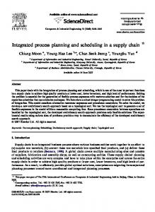
Figure 1: Example of Action Graph for a purely propositional ground operator “MoveATableB” in the Blocks World domain. Definition 3. An Action Graph is a tuple hP, E, A, Ci, where • P is a set of Temporal Assertions which represent the preconditions for applying the operator. • E is a set of Temporal Assertions which represent the effects of applying the operator; • A is a set of Temporal Assertions to be asserted as a consequence of the application of the operator (and that are neither preconditions nor effects); • C is a set of temporal constraints between pairs of TAs in P ∪ E ∪ A. • An AG is associated with a flexible temporal duration, implied by C. Preconditions (effects) are constrained to start (finish) at the beginning (end) of the AG’s temporal extension. An AG can be used to represent a temporally-rich causal operator by modeling preconditions, effects and all TAs in A as PTAs. Notice, though, that preconditions, effects and all other TAs modeled in the AG may be STAs or RUTAs as well. This entails that the assertions implied by the execution of a set of concurrent AGs may conflict in ways that are not deducible by a purely propositional planning procedure. In order to refer to the purely propositional fragment of an AG, we extend the concept of propositional projection defined earlier for PTAs. Specifically, PTAs in the preconditions and effects of an AG subsume the propositional preconditions and effects of a ground STRIPS-like operator: Definition 4. Given an AG hP, E, A, Ci, the propositional projection V of its preconditions (effects) is a predicate logic formula ptai pi , where ptai = hxi , vi , [Is , Ie ]i ∈ P (∈ E) is a P T A, pi = xi if vi = > and pi = ¬xi if vi = ⊥. In the remainder of this article we refer to the propositional projection of an AG’s preconditions and effects with the notations prop(P) and prop(E). Example 2. An example of AG in the propositional Blocks World domain is shown in Figure 1. The AG describes the operation of moving block A from the table to block B, and states in detail the temporal relationships that exist between the PTAs that model the operation. Preconditions include, for instance, that block A should be on the table. The

AG also models the temporal constraints that should exist among PTAs. For instance, the precondition that block A is on the table meets temporally the effect that A is no longer on the table. Also, notice that the AG models as PTAs also predicates that should hold during the interval of time in which the operation is being executed, and that are neither preconditions nor effects (e.g., that block A is not free while it is being handled by the robotic arm). In order to better visualize the structure of the AG, one can observe the timelines of the variables involved. Figure 2 sketches the timelines of the five predicates used in the Blocks World AG example above. The timeline view shows clearly that the AG induces two or more flexible temporal intervals on each logical proposition, namely an interval in which preconditions should hold, one in which effects should hold, and one interval (but in general any number of intervals) in which assertions that have no consequence on the causal theory should hold. OnAB OnATable

⊥ (P) > (P)

FreeA > (A) FreeB

⊥ (A)

> (A)

MoveATableB ⊥ (A)

> (E) ⊥ (E)

> (A)

> (A) ⊥ (E) ⊥ (A) time

Figure 2: Timelines of the five predicates employed to model the AG in Example 2.

Note that in Example 2 we have omitted specifying the bounds of the constraints in C. In general, specifying precise bounds on these constraints allows to fine-tune the model to reflect realistic execution conditions. For instance, the constraint hOnAB, >, [Is , Ie ]i OVERLAPS [2, 5] hMoveATableB, >, [Is0 , Ie0 ]i models the fact that the precondition OnATable remains true for at least two and at most five time units after the beginning of the MoveATableB operation. Henceforth, when omitted, we assume that bounds on constraints are [0, ∞). AGs are the basic building block of a planning and scheduling problem instance. They are employed in our architecture to express a domain which, as a consequence of the general nature of TAs, is not necessarily a purely causal domain, and can describe causal, temporal, and resourcerelated aspects of the real world problem we wish to solve. More specifically, Definition 5. An integrated planning and scheduling problem is a tuple hV, O, I, Gi, where • V = Vp ∪ Vs ∪ Vr is a set of variables, partitioned into three sets representing, respectively, predicates, state variables and renewable resources; • O is a set of AGs representing operators whose preconditions, effects and temporal assertions are defined over the variables in V; • I is a set of TAs representing the initial condition; • G is a set of TAs representing the goal; Note that the propositional projection of the initial condition prop(I) is a predicate logic formula over the predicates

in Vp which represents the initial state of a purely propositional planning problem (the same holds for the goals G). This problem thus represents a relaxation of the integrated planning and scheduling problem.

4

Search in the Space of Causal Epochs

Our architecture performs search in the space of what we call causal epochs. A causal epoch is a collection of AGs enclosed by a flexible interval to which preconditions and effects are temporally constrained. Specifically, Definition 6. A causal hΛ, Sb , Se , [Is , Ie ] , Ci, where

epoch

is

a

tuple

• Λ = {hP1 , E1 , A1 , C1 i, . . . , hPn , En , An , Cn i} is a set of Action Graphs; [ • Sb = Pi is the beginning state of the causal epoch; Λ

• Se =

[

Ei is the end state of the causal epoch;

Λ

• [Is , Ie ] is a flexible interval representing the temporal extension of the epoch; • C is a set of constraints that bound each precondition in Sb (effect in Se ) to STARTS-WITH (ENDS-WITH) Is (Ie ). Note that all preconditions of the AGs in Λ are constrained to start at the lower bound of the epoch, while all effects are constrained to end at the upper bound of the epoch. Similarly to levels in a planning graph (Blum and Furst 1997), levels of epochs represent causal steps in the plan. However, since AGs have a non-unit temporal dimension, the temporal extension of an epoch can be quantitatively bounded. The sets Pi , Ei , Ai and Ci of the AGs in a causal epoch define a constraint network which models causal precedence as well as other temporal and resource requirements. Thanks to the temporal flexibility maintained within the scope of a causal epoch, it is possible to delegate temporal propagation and any resource/state variable conflicts that may exist between TAs in the epoch to OMPS’s temporal reasoning and scheduling modules. As we will see shortly, this is the core factor that enables tightly-coupled planning and scheduling. The beginning and end states of a causal epoch represent the predicates that hold in a sampled instant of time corresponding, respectively, to the lower bound or the upper bound of the causal epoch. Specifically, Definition 7. Given a causal epoch hΛ, Sb , Se , [l, u] , Ci, theVpropositional projection of its beginning (end) state is a ptai pi , where ptai = hxi , vi , [Is , Ie ]i ∈ Sb (∈ Se ) is a P T A, pi = xi if vi = > and pi = ¬xi if vi = ⊥. Henceforth, we refer to the propositional projection of a causal epoch’s beginning and end states as prop(Sb ) and prop(Se ). The initial conditions and goals are given to a causal reasoning module which operates similarly to GraphPlan. The planning procedure considers a relaxation of the original integrated planning and scheduling problem. This relaxation does not occur strictly along the separation between the causal and temporal/resource aspects of the problem, as there are causal dependencies that are not considered by the causal reasoning module and delegated to the

scheduler, as well as scheduling-related aspects that are considered by the causal reasoning module by means of newly defined mutex relations (explained below). The causal reasoning module performs essentially two tasks. First, it performs backward chaining over the beginning and end states of causal epochs. The applicability of an AG given the current state is a purely causal matter: Definition 8. An AG hP, E, A, Ci is applicable to the end state Se (resp., beginning state Sb ) of a causal epoch if prop(Se ) |= prop(E) (resp., prop(Sb ) |= prop(P)). Second, the causal reasoning module propagates also noncausal constraints related to resource usage. The result of the causal reasoning module’s inference are relaxed plans which are then refined by a scheduling module until scheduling conflicts in all the epochs have been resolved. If resolution of these conflicts cannot be performed, the causal reasoner will return a new plan which takes into account the conflicts identified by the scheduler. The plans resulting from the integrated planner and scheduler are sequences of causal epochs in which all causal and scheduling conflicts have been resolved, and whose concatenation through the propositional projections of end/beginning epoch states brings from an initial situation to the goal. More specifically, Definition 9. Given a planning problem hV, O, I, Gi, a plan is a sequence {hΛ1 , Sb1 , Se1 , [Is1 , Ie1 ] , C1 i, . . . , hΛn , Sbn , Sen , [Isn , Ien ] , Cn i} of causal epochs such that • prop(Sb1 ) |= I and prop(Sen ) |= G; • prop(Sbi ) |= prop(Sei−1 ); • all temporal, symbolic and resource conflicts have been resolved. The coordination and communication between the causal reasoning module and the scheduler are detailed in Function Plan. The algorithm starts by invoking the causal reaFunction Plan(O,I,G): plan π or failure 1 2 3 4 5 6 7 8 9 10 11 12 13 14 15

π ← empty plan; mutexSet ← ∅ while true do relaxedPlan = {Ω1 , . . . , Ωl } ← CRM (O, I, G, mutexSet) if (relaxedPlan = ∅) then return failure conflict ← false while (relaxedPlan 6= ∅ ∧ ¬ conflict) do Ω = {hP1 , E1 , A1 , C1 i, . . . , hPn , En , An , Cn i} ← Pop(plan) S S S Λ ← Ω; Sb ← Ω Pi ; Se ← Ω Ei ; C ← Ω C E ← hΛ, Sb , Se , [Is , Ie ] , Ci C 0 ← SM(E) if SchedulingConflict(E) then mutexSet ← Ω π = ∅; conflict ← true else C ← C ∪ C 0 ; π ← π.E if (¬ conflict) then return π

soning module (CRM) to obtain a candidate relaxed plan (line 3). This plan is a sequence of sets Ωi ∈ 2ω∪η , where ω is a set of AGs, and η is a set of no-ops (defined in the next

section). Each set Ωi represents a “plan step”, i.e., a selection of domain operators and no-ops to satisfy the open goal in the ith level of the planning graph. These operators are non-interfering and therefore they can be executed concurrently (as far as the causal reasoning module can ascertain.) All AGs and no-ops in a plan step Ωi are instantiated to obtain a new causal epoch. The algorithm instantiates a new epoch for each plan step in the relaxed plan, starting from the last plan step Ωn (lines 7–9). Each epoch so obtained is then checked for scheduling conflicts by the scheduling module (SM). The scheduler deduces, if possible, a set of precedence constraints that solve these conflicts (line 10). In the event of success (line 14), the scheduler has thus refined the causal epoch E with (only the necessary) constraints that decrease the concurrency of AGs in Ωi as it was determined by the causal reasoning module. It appends the epoch E to the current plan π and each Ωi in the plan is processed. In the event of a failure by the scheduler to find a solution for the conflicts in an epoch, the cycle is interrupted (lines 11–13) and the causal reasoning module is re-invoked to generate an alternative plan (line 3). Notice that at this point, a non-empty mutexSet is provided to the causal reasoning module representing the epoch that has caused the failure. Specifically, this constitutes an indication as to which choice of operators and no-ops should be avoided in the search for another plan by the causal reasoning module (a process similar to memoization in GraphPlan).

4.1

Causal Reasoning Module

The use of a causal reasoning module loosely based on GraphPlan allows us to maximize the “logical concurrency” in the plan through the use of a level-directed search in which sets of AGs lead from one propositional level to the next. The search mechanism employs mutex relations which are weaker than classical GraphPlan mutexes. Moreover, as opposed to GraphPlan, where a graph is expanded forwards until goals appear non-mutex, we search while expanding backwards from the goals, as suggested in (Haslum and Geffner 2000). Furthermore, frame axioms are “encoded” into special “no-op AGs” which prolong the value of a predicate, resource or state variable as well as the consequences it implies throughout an entire epoch: Definition 10. A no-op is an AG hP, E, ∅, Ci such that • P = E contains a PTA representing the assertion that is to be extended throughout the causal epoch; • C is a set of EQUALS constraints among the TAs in P which enforce all TAs to occur concurrently. In our approach, mutexes leverage the presence of resource-related information in the problem, and state weaker criteria for assessing whether operators should be logically exclusive. Specifically, 1. Two AGs hP, E, A, Ci and hP 0 , E 0 , A0 , C 0 i are mutex if one of the following two conditions hold: a. prop(P) |= ¬prop(P 0 ) or prop(E) |= ¬prop(E 0 ); b. Given a reusable resource x with capacity Cx , ∃r = hx, vi ∈ P(or E) and ∃r0 = hx0 , v0 i ∈ P 0 (or E 0 ) such that x = x0 and v + v0 > Cx .

2. An AG hP, E, A, Ci and a no-op hP 0 , E 0 , ∅, C 0 i are mutex if one of the following two conditions hold: a. prop(P) |= ¬prop(P 0 ), or prop(E) |= ¬prop(P 0 ), or prop(A) |= ¬prop(P 0 ); b. Given a reusable resource x with capacity Cx , ∃r = hx, vi ∈ (P ∪ A ∪ E) and ∃r0 = hx0 , v0 i ∈ P 0 such that x = x0 and v + v0 > Cx . Rules (1a) and (2a) identify purely propositional conflicts. These mutexes are a subset of those detected by the GraphPlan algorithm, since they do not single out mutually exclusive concurrent actions with interfering effects. This absence permits to include plans in which two or more actions at the same level (i.e., in the same epoch) jointly achieve an overall effect while deleting each others’ preconditions. In the Blocks World domain for instance, this allows to model operators that achieve, in one causal epoch, an “exchange” of blocks between different piles. Given that our planner can deal with resources, it is natural to provide the domain modeler with this possibility, as we can model a “manipulator” resource with capacity two, meaning that the manipulation subsystem of the corresponding real-world problem is capable of handling two blocks at a time (e.g., through the use of two robotic arms). Indeed, in our approach it is the scheduling module that is responsible for verifying the soundness of the behavior of concurrent actions in Ω with respect to temporal and resource related aspects. As opposed to GraphPlan, we provide rule (1b) which takes into account the joint resource requirement of the preconditions or effects of two operators. This constitutes a simple form of resource propagation, where we check for resource feasibility in sampled instants of time (the beginning states of causal epochs) in which we are sure that resource usage assertions (RUTAs) will be concurrent. Notice that we can be sure that there will be temporal concurrency between RUTAs in an operator with any RUTA in a no-op, as a no-op represents invariant conditions in time, e.g., a noop may involve the constant requirement u of a reusable resource x during an entire epoch; if such a no-op exists in the causal epoch, any other RUTA requiring more than Cx − u of the same resource x induces an inconsistent state. Overall, all temporal constraints and TAs in an epoch together entail potentially concurrent resource usage (in the case of RUTAs), symbolic assertions (in the case of STAs) or predicates (in the case of PTAs). The causal reasoner “filters” some of the possible contentions caused by this concurrency in each epoch. Those that remain are discovered and solved by the scheduling module, which, in case of failure, returns an indication as to which concurrent selection of AGs and no-ops have caused the unresolvable conflict. These indications are interpreted again as mutual exclusions during search, albeit of a higher order, and are taken into account by the backwards planning graph exploration in an attempt to generate a new relaxed plan.

5

Causal Conflicts and Scheduling

As explained, the causal reasoning module solves a relaxed problem in which only some conflicts have been taken into consideration. This leaves the freedom, at modeling time, to

choose which aspects of the domain should be cast as conflicts to be processed by the causal reasoning module, and which should instead be cast as scheduling conflicts for consideration by the scheduling module. In addition, given the flexibility in defining conflicts through contention on predicate values and resources, the domain modeler can choose the specific semantics of concurrency (Cayrol, R´egnier, and Vidal 2001) to model into the operator descriptions. On one hand, s/he can follow a “classical” approach, where the conflicts to be identified correspond to those that would be mutexes in a traditional GraphPlan approach. On the other, the modeler can leverage the increased expressiveness afforded by reusable resources, using temporally-bounded RUTAs to limit the executability of operators. To show this spectrum of possibilities, we illustrate two alternative formulations of the Blocks World domain in the specific context of solving the Sussman Anomaly. 0 1 2 3 4 5 6 7 8 9 10 ⊥

OnAB

OnCA

>

⊥

OnBC

> ⊥

>

⊥

⊥

OnCTable RFreeA

>

⊥ >

OnBTable

>

>

>

OnATable

0 1 2 3 4 5 6 7

> >

>

1

>

1

1

RA

1 ⊥

1

>

FreeA > RFreeB

1

⊥

1

> 1

RB

1 >

⊥

1

>

FreeB > RFreeC

1

1

⊥

1

RC

1 >

⊥

1

>

FreeC >

⊥

⊥

MoveATableB MoveBTableC

⊥

MoveCATable ⊥

>

> >

⊥

>

⊥ ⊥

Classical formulation

> >

Resource formulation

Figure 3: Timelines representing the two final plans for the Sussman Anomaly. The arrows indicate temporal precedence constraints imposed by the scheduling module. Classical formulation. Figure 3 (left) shows the final plan obtained with our architecture in the case of a domain representation which tightly follows the classical formulation of the Blocks World operators (for reasons of space, we omit the full description of the AGs in this domain). The operators involved are MoveCATable, MoveBTableC and MoveATableB. As shown, the three operators model as preconditions and effects the some of the predicates one would find in a classical STRIPS formulation of the blocks world domain (see the highlighted PTAs for the AG “MoveCATable” in the figure), e.g., block C is on the table before the action MoveCATable, a condition which ceases to be true after the action. In addition, given the greater temporal flexi-

bility afforded by our system and domain representation formalism, operators also establish conditions that should hold between the epoch’s temporal bounds, e.g., FreeB is false during the execution of operator MoveBTableC but true before and after. More importantly, the example shows how “classical” causal conflicts can be reasoned upon by the scheduling module. Specifically, the solution to the Sussman Anomaly requires the scheduler to impose a sequence between conflicting, concurrent predicate values. For instance, hFreeA , ⊥, ·i would contradict hFreeA , >, ·i between time t = 0 and time t = 1, if the scheduler had not imposed the precedence constraint between these two PTAs. In addition, the classical formulation employs simple binary resources to “protect” against illegal concurrent transitions in truth values. For instance, operator MoveBTableC prescribes among its TAs in A that there exists an interval of time between the assertion hFreeB, ⊥, ·i and the assertion hFreeB, >, ·i in which a RUTA hRFreeB , 1, ·i uses one unit of a reusable resource RFreeB whose capacity is one. All operators asserting values on the predicate FreeB assert an equivalent RUTA on RFreeB when the value is flipped. As a consequence, an over consumption of resource RFreeB will occur every time any two of these RUTAs overlap in time. This, in turn, will prompt the scheduling module to impose temporal constraints that solve these conflicts. All the constraints imposed by the scheduler are highlighted in the figure; they determine the temporal placement of the operators, namely that MoveATableB must follow MoveBTableC, which must follow MoveCATable. The above formulation suggests a general technique to formulate STRIPS operators in our architecture. This technique essentially consists in reducing the problem of ensuring consistent changes of predicates along the timeline to the problem of verifying the concurrent access to shared variables by processes. These variables are binary resources over which “consuming” assertions must be synchronized. It is interesting to note that the classical formulation is in some ways similar to the S TRIPS L INE approach described in (Cesta and Fratini 2008). S TRIPS L INE, however, hinges on action/predicate representations that are instantaneous. Furthermore, the S TRIPS L INE planner solves a timelinebased formulation of a classical planning problem rather than an integrated planning and scheduling problem. Resource formulation. While the classical formulation has enabled us to enrich the classical Blocks World planning problem with temporal flexibility, it drastically under-uses the potential offered by the sophisticated resource reasoning algorithms in OMPS’s scheduling module. Indeed, many classical planning problems implicitly state resource usage aspects of the domain in the logical propositions they assert. Our architecture allows to assert resource consumption explicitly and in a quantified way through RUTAs. This allows to compactly model those resource-related features of classical planning problems that are typically “compiled away” into propositional operator specifications. Figure 3 (right) shows the plan obtained with an alternative formulation of the operators. This formulation employs reusable resources of capacity 1 to represent the spatial af-

fordance of each block: RBlockA , RBlockB and RBlockC . In addition to logical preconditions and effects, AGs assert usage of these resources in a very natural way, whereby the “move” operators assert usage of the block resources. Specifically, the AG for moving block A from the table to block B is specified as follows (highlighted in the figure): hMoveATableB, >, ·i MEETS hOnAB, >, ·i hOnAB, >, ·i EQUALS hRB , 1, ·i hOnATable, >, ·i OVERLAPS hMoveATableB, >, ·i hMoveATableB, >, ·i EQUALS hRA , 1, ·i

The RUTAs on reusable resources directly enable a scheduler-based conflict resolution mechanism for interfering effects, because AGs explicitly assert when a resource is free, and therefore when it can be allocated to other activities. This example underscores an important added value of the least commitment propositional conflict resolution strategy employed in the causal reasoning module, namely increased concurrency. The result is a plan in which the three operators partially overlap thanks to the temporal constraints binding the “move” and “on” PTAs with the RUTAs asserted on the resources. Overall, the ability to model operators which depend on resource usage as well as logical assertions provides an intuitive way to model some very significant aspects of the domain — the space on top of a block is such an aspect in our example. As we show in the next section, this type of formulation brings with it a strong computational advantage. Moreover, the presence of multi-capacity reusable resources also entails a representational advantage. In our Blocks World, for instance, the only change in the domain description we need to implement in order to accommodate blocks of different sizes is to increase the capacity of the resources modeling the blocks, and to change the value of the RUTAs in the AG descriptions accordingly. Finally, notice that in both formulations the integrated planner and scheduler has solved the Sussman Anomaly in a single causal epoch. Within this epoch, we can notice that the solution in the classical representation is actually “layered”, in a similar fashion as a plan generated by classical GraphPlan would be. The fact that “GraphPlan-like” causal conflicts have been correctly identified within one epoch is an indication of the extent to which the scheduling module also resolves causal conflicts which have been modeled in the operator descriptions. As testified by the solution in the resource formulation, it is possible to leverage these less committed relaxed plans more effectively by specifying domains that make a more intelligent use of resources.

6

Evaluation

In this section we propose an experimental validation of our system based on two benchmarks in the Blocks World domain. The first benchmark consists of 12 problem instances, all of which are variants of the same base problem. This is the worst possible case for the Blocks World domain, namely that in which the goal is to stack the block on the bottom of a stack on top of it — e.g., going from (A over B

Classical form. # blocks

CRM (SM)

3 4 5 6 7 8

540 (472) 1405 (4721) 4473 (27724) 15296 (169932) 75234 (844317) 767463 (348850)

Resource form. # MCS 10 27 63 134 286 598

CRM (SM)

# MCS

306 (22) 397 (128) 555 (525) 1039 (2058) 4060 (10134) 48155 (39912)

1 2 4 7 13 23

Table 1: Performance of the system with classical vs. resourcebased formulation (all times are in milliseconds).

over C) to (C over A over B). Any solution requires exactly two causal epochs, as it is possible to go from one configuration to any other configuration of blocks by (1) unstacking all blocks and putting them on the table, and (2) stacking them again in the desired order. Both operations require one epoch. Conversely, in problems like the Sussman Anomaly, or “completely inverting a stack” for that matter, the desired configuration can be achieved in the same epoch if unstacked blocks are put directly in the desired position. The 12 problems used for the benchmark are partitioned in two sets of 6 instances each. The ith instance in one set expresses exacly the same problem as the ith instance in the other set, their difference being only the formulation: in the first set, all instances are expressed using the classical formulation, while in the second they are expressed using the resource formulation. Each group of 6 instances is a variation of the base problem described above with an increasing number of blocks (from three to eight). The results of this first batch of experiments are reported in Table 1. As expected, the resource-based formulation leads to a large improvement in performance compared to the classical formulation. This is due to several factors. First, AGs are represented more compactly in the resourcebased formulation. This entails a lower burden for the temporal reasoning module (on which the scheduling module is based), as fewer timepoints require processing. Temporal constraint propagation is called into play every time a constraint is added or removed, and thus occurs many times during scheduling. As a result, even in the largest problems, the gain in computation time for the scheduling module (SM in the table) is of an order of magnitude. Second, it is evident from the results that the classical formulation over-burdens the causal reasoning module (CRM in the table). Specifically, the resource-based formulation entails that less binary mutex relations need to be deduced by the CRM. Finally, the table shows the number of Minimal Critical Sets (MCS, (Laborie and Ghallab 1995)) analyzed by the SM while solving scheduling conflicts. The number of MCSs provides a measure of the “amount of scheduling” performed by the system, as it is directly related to the number of resource contentions present in the problem. Notice that in the classical formulation, we are actually performing more scheduling as a result of the many concurrent PTAs representing logical assertions on whether blocks are free, whether they are stacked on top of each other, etc. Indeed, in defining the AGs according to a resource-based formulation, we are employing resource conflicts to drive the search away from complex propositional inference. The SM can in-

# blocks 3 4 5 6 7 8

Resource form. CRM (SM) # MCS 128 (11) 1 896 (74) 10 6352 (2165) 167 25096 (9180) 595 574427 (173255) 12543 1629534 (311684) 27189

Table 2: Performance of the system on a multi-capacity Blocks World domain (all times are in milliseconds).

deed be made to perform this type of inference, as shown by the classical, STRIPS-like formulation, where the scheduler bears the brunt of temporally de-coupling conflicting predicate values. However, the SM is more informed if driven only by conflicts on resources, whose expressiveness allows to subsume many aspects of the problem at hand. The second benchmark consists in six problem instances in which blocks can have non-unit sizes. As remarked above, this can be achieved by using the resource formulation. For each problem (n blocks), dn/2e blocks have capacity two (meaning that it is possible to stack two blocks of capacity one over them), while the rest have capacity one; the initial state is a vertical stack (with large blocks on the bottom), and the goal state consists in placing all large blocks on the table and all small blocks on top of the large ones. The results (Table 2) show an interesting difference when compared to the previous benchmark. In fact, despite the apparently simpler structure of the problems (which can be solved in one epoch, as opposed to the two necessary to solve the previous benchmark problems), the performance of the system, both in terms of the CRM and in terms of the SM, is much worse. This is due to the increased capacity of the resources modeling blocks. The higher capacity of these resources entails that there are less binary mutexes that the CRM can use to discard invalid relaxed plans. Furthermore, these plans ultimately constitute causal epochs whose search space is less constrained, therefore inducing the scheduler into more conflict resolution cycles. This last point is evident in the drastically larger number of MCSs in the second benchmark compared to the first one.

7

Related Work

Many approaches to the planning and scheduling integration problem have been explored, ranging from loosely-coupled integrations of a planner and a scheduler (Pecora and Cesta 2005), to more tight integrations. Among the latter, we can distinguish “homogeneous” approaches like (Penberthy and Weld 1994), whereby both planning and scheduling subproblems are reduced to a common reduction. These approaches, however, often fail to scale up due to difficulty to use strategies that are specific to causal, resource and temporal aspects of the problem. Other approaches based on constraint reasoning have also been reported, e.g., IxTeT (Ghallab and Laruelle 1994) and the EUROPA/RAX-PS planning approach developed at NASA (J´onsson et al. 2000). The former adheres to a different planning paradigm (HTN as opposed to STRIPS-like), and both search for a solution by exploring possible resolutions of flaws in the plan. Conversely, our approach relies on the more “classical” principle of op-

erator chaining. As a consequence, our system can employ more effective heuristics for causal reasoning (as opposed to problem-dependent, hand-crafted heuristics). Also, notice that our system retains an advantage of both IxTeT and the NASA approach, namely the notion of iterative refinement through the use of specialized reasoning procedures. Acknowledgements. The authors wish to thank Alessandro Saffiotti, Giuseppe De Giacomo and Marcello Cirillo for their support and useful insights.

References Allen, J. 1984. Towards a general theory of action and time. Artif. Intell. 23(2):123–154. Blum, A., and Furst, M. 1997. Fast planning through planning graph analysis. Artificial Intelligence 90(1–2):281– 300. Cayrol, M.; R´egnier, P.; and Vidal, V. 2001. Least commitment in graphplan. Artif. Intell. 130(1):85–118. Cesta, A., and Fratini, S. 2008. The Timeline Representation Framework as a Planning and Scheduling Software Development Environment. In Proc. of 27th Workshop of the UK Planning and Scheduling SIG. Cesta, A.; Oddi, A.; and Smith, S. F. 2002. A constraintbased method for project scheduling with time windows. Journal of Heuristics 8(1):109–136. Dechter, R.; Meiri, I.; and Pearl, J. 1991. Temporal constraint networks. Artif. Intell. 49(1-3):61–95. Fratini, S.; Pecora, F.; and Cesta, A. 2008. Unifying Planning and Scheduling as Timelines in a Component-Based Perspective. Archives of Control Sciences 18(2):231–271. Ghallab, M., and Laruelle, H. 1994. Representation and Control in IxTeT, a Temporal Planner. In Proc. of the 2nd Int. Conf. on Artif. Intell. Planning and Scheduling. Haslum, P., and Geffner, H. 2000. Admissible Heuristics for Optimal Planning. In Proc. 5th Int. Conf. on AI Planning and Scheduling, 140–149. J´onsson, A.; Morris, P.; Muscettola, N.; Rajan, K.; and Smith, B. 2000. Planning in interplanetary space: Theory and practice. In Int. Conf. on Artif. Intell. Planning and Scheduling, 177–186. Laborie, P., and Ghallab, M. 1995. Planning with Sharable Resource Constraints. In Proc. of the 14th Int. Joint Conf. on Artif. Intell. Pecora, F., and Cesta, A. 2005. Evaluating Plans through Restrictiveness and Resource Strength. In Proc. of the 2nd Workshop on Integrating Planning into Scheduling at AAAI-05. Penberthy, J., and Weld, D. 1994. Temporal planning with continuous change. In Proc. of the 12th Nat. Conf. on Artif. Intell., 1010–1015. Vilain, M.; Kautz, H.; and van Beek, P. 1989. Constraint propagation algorithms for temporal reasoning: A revised report. In Weld, D., and de Kleer, J., eds., Readings in Qualitative Reasoning about Physical Systems, 373–381. Morgan Kaufmann.