A CONSTRAINT-BASED SCHEDULING OF OFFSHORE WELL DEVELOPMENT ACTIVITIES WITH INVENTORY MANAGEMENT Thiago Serra Instituto de Matemática e Estatística – Universidade de São Paulo Rua do Matão, 1010 – Cidade Universitária – São Paulo – SP – Brasil – CEP: 05508-090
[email protected] Gilberto Nishioka Departamento de Engenharia Química – Escola Politécnica – Universidade de São Paulo Av. Prof. Lineu Prestes, 580 – Cj. Quimicas Bl.18– São Paulo – SP – Brasil – CEP: 05508-970
[email protected] Fernando J. M. Marcellino PETROBRAS - Tecnologia da Informação São Paulo Av. Paulista, 901 – 4o andar – São Paulo – SP – Brasil – CEP: 01311-100
[email protected]
S I A
ABSTRACT This work aims at proposing and tackling a novel version of the resource scheduling problem to perform exploitation activities in offshore oil wells. It differs from previous approaches for considering inventory issues related to the transportation of lines that connect wells to the surface. The Constraint Programming (CP) technique was used this time due to late improvements in state-of-art constraint modeling that facilitated prototyping and also due to the improvement of CP solving mechanisms for scheduling. An algorithm for upper bound estimation is also presented to assess the quality of the obtained solutions. The resulting scheduler was tested with real data from PETROBRAS and it will be further improved to be used by this company very soon.
N A É
KEYWORDS. Oil Well Development, Scheduling, Constraint Programming. Main area. P&G – O.R. in Oil & Gas Applications.
R P
RESUMO Este trabalho visa propor e abordar uma nova versão do problema de alocação de recursos para a realização de atividades de produção em poços de petróleo marítimos. Ele difere de abordagens anteriores por contemplar questões de estoque relativas ao transporte de linhas que conectam os poços à superfície. A técnica de Programação por Restrições (PR) foi usada devido a melhorias recentes nas ferramentas de modelagem com restrições que facilitaram a prototipagem e também devido à melhoria dos mecanismos de resolução de PR para problemas de escalonamento. Um algoritmo para a obtenção de um limitante superior é também apresentado para avaliar a qualidade das soluções obtidas. O escalonador resultante foi testado com dados reais da PETROBRAS e será aperfeiçoado para o uso por esta empresa em breve. PALAVRAS CHAVE. Desenvolvimento de Poços, Escalonamento, Programação por Restrições. Área principal. P&G – PO na Área de Petróleo & Gás.
PRÉ-ANAIS XLIIISBPO
1. Introduction Exploitation activities are related to the development of new oil wells and the maintenance of the existing ones. They must be performed by scarce resources such as oil rigs and linelay vessels. Those resources are required to operate over a wide geographical area and are subject to predicted downtimes related to their routine maintenance. Each well starts producing oil as soon as its development activities are concluded. The schedule of their development is intended to maximize the resulting short-term gain in oil production. Besides, exploitation activities are much more detailed than the exploratory ones that precede them, as described by Glinz and Berumen (2009). Therefore, this problem assumes a critical role due to its closeness to the operational level in one of the most expensive processes of oil companies value chain. On account of the amount of wells and resources managed by the company under study, it takes days to find a scheduling solution manually and optimization is barely considered. It is noticeable that unexpected events such as activity delays and resource breaks may invalidate the whole schedule. Moreover, any tactical analysis to acquire more resources requires a comparison between schedules with and without them. Hence, exploitation scheduling represents a situation in which automatization is mandatory and optimization would provide a competitive edge. This problem has already been tackled by many approaches since its inception by Hasle et. al. (1996). It was shown by Nascimento (2002) that it is NP-hard since it is as hard as the JobShop Scheduling problem, what means that it is not known an efficient algorithm for the general case of the problem. Several of these previous approaches represent a progressive detail of a single specification, including Nascimento (2002), Accioly et. al. (2002), Pereira et. al. (2005) and Moura et. al. (2008). Techniques such as Constraint Programming (CP) and metaheuristics like Greedy Randomized Adaptive Search Procedures (GRASP) and Tabu Search (TS) have been used to some extent in previous works. CP was first used by Accioly et. al. (2002) and compared to GRASP in Pereira et. al. (2005), where it was slightly outperformed. There are also approaches to related problems in the life-cycle of oil reservoirs such as resource planning for exploration activities by Glinz and Berumen (2009) and scheduling routine maintenance on wells that are already producing. Paiva (1997) tackled the maintenance of offshore wells whereas Aloise et. al. (2006) tackled onshore wells. Nevertheless, there are some subtleties in real-life exploitation scheduling yet to be considered in order to achieve a solution that is truly applicable. This work presents an augmented description of the problem and a novel approach to tackle it. Such amend to the problem description refers to the inclusion of inventory restrictions of linelay vessels. Those resources are responsible for the load of lines at harbors and their release at developing wells in order to trigger oil production. The approach to the problem consists of a declarative formulation aimed at facilitating the problem resolution by means of a commercial CP solver. An algorithm that provides an estimation of the optimality gap to assess the quality of the obtained solutions is also introduced. Thus, our intent is to give further insight about the problem and to explore current capabilities of the CP technology for scheduling problems as well. The organization of the remainder of the text is as follows. A description of the problem is presented in section 2. The approach to the problem is presented in section 3 along with an introduction to the CP technique and to the syntax in which the problem is then formulated. The algorithm for upper bound estimation is described in section 4. Some experimental results are exhibited in section 5 and subsequently discussed in section 6. Final remarks are presented in section 7.
R P
N A É
S I A
2. Problem The exploitation scheduling problem can be depicted as a matter of deciding if, when and how to perform each of several activities associated with wells or harbors using a given set of resources. Time is discretized in days, starting from a given date represented by 0. For notational convention, resources will be denoted by the index i, ranging from 1 to nr ; activities by j, ranging from 1 to na with the first nw activities performed on wells and the remainder on harbors; and sites, both wells and harbors, by k. In what follows, such indexes are used to represent the
PRÉ-ANAIS XLIIISBPO
problem details. 2.1. Optimization criteria The main objective is to maximize short-term production of the schedule, which is a measure of how much each well would produce since the day its development finishes until a given date H. Each activity j is supposed to have an associated daily production rate pj once it is concluded, which is nonzero only in the case of the last activities on each well. Secondarily, it is also pursued to anticipate the conclusion of each activity in the schedule. 2.2. General resource restrictions – – – – – – –
Each resource performs only one activity at a time. Each resource i has a contract period from day csi to day cei , out of which it is unavailable. During that contract period, there are predicted resource outages. These outages are periods in which no activity can be performed by the resource. A resource can perform only activities whose requirements are compatible with its features. Let cij = 1 if and only if resource i and activity j are compatible. Only one resource can be assigned to a well at any time. In order to use a resource to perform consecutive activities at different sites, it is necessary to consider the time to move that resource from a location to another. Some resources are not allowed to get closer than a given distance to each other due to the collision risk.
2.3. General activity restrictions – – – – – –
Once an activity starts, it is performed non-stop until conclusion. Each activity j has pre-defined early and late starting dates, denoted by esj and lsj . Each activity j is associated with a site sitj . For activities on wells, the duration is fixed and given by dj . One activity may be preceded by other activities, each of which demanding a minimum time interval from the end of one to the start of the other. Some activities may belong to a cluster, in which all activities should be performed by a single resource.
R P
2.4. Inventory restrictions – – –
– – – –
– –
S I A
N A É
Each resource starts the schedule with an empty inventory. Each resource i has a maximum inventory capacity ici , which is nonzero only for linelay vessels. Only resources with positive inventory capacity may perform loading activities at harbors. Each harbor k may support up to sk simultaneous loading activities. A loading activity performed by a resource i lasts from mili up to mali days. The increase of the onboard inventory due to a loading activity is proportional to the time it lasts, and a resource i increases its inventory by ici after mali days. In order to perform an activity j that involves line connection, a resource must have the necessary line weight wlj to unload there. Loading activities are not subject to cluster or precedence constraints. The number of loading activities is not predetermined. However, it is possible to set an upper limit as the product of the number of harbors by the number of connection activities.
3. Approach Our approach to the problem is based on the CP technique or, more specifically, on Constraint-Based Scheduling (CBS). The problem of study was formulated to be tackled with a
PRÉ-ANAIS XLIIISBPO
CBS solver using the concept of interval variables. In what follows, some notions about CP and CBS as well as about interval variables formulation are given prior to the CP model itself. 3.1. CP and Constraint-Based Scheduling CP is defined by Lustig and Puget (2001) as a computer programming technique in which combinatorial problems are formulated using constraints designed to capture problem structure more easily. These constraints make it possible to infer domain reductions involving the decision variables of the problem so that search space is pruned before and during search, what is described by Barták (2001) as constraint propagation. In addition, its search techniques are based on backtracking and local search algorithms that are possibly biased by problem structure, according to Beek (2006) and Godard et al. (2005). With the advent of algebraic modeling languages supported by CP solvers, Lustig and Puget (2001) regarded that the technique was no longer restricted to computer programming experts and it was possible to use it in the development of abstract formulations suitable for direct execution in these solvers. It is noticeable that CP strength is due to how it can handle specificities of application domains, usually by means of global constraints. Bessière and Hentenryck (2003) observe that a global constraint represents a complex but common relation among a set of variables, for which more efficient propagation algorithms are designed. Scheduling is a special case in which CP is very competitive, what led to the development of CBS. CBS is a specialization of CP towards scheduling problems, whose competitiveness is due to the fact that scheduling problems usually require linear formulations whose size prevents them from being solved with Mixed-Integer Programming (MIP) algorithms in reasonable time with available hardware resources. For a comprehensive introduction to CP and to CBS, the interested reader is referred to Dechter (2003) and Baptiste et. al. (2001), respectively.
S I A
3.2. Formulation syntax Interval variables represent an expressive generalization of abstractions such as activities and resources for modeling scheduling problems. Each interval variable depicts an event through a collection of interdependent properties such as its occurrence, starting date, duration and ending date. Those properties will be denoted by the following functions over the interval given as argument, respectively: occur, start, duration and end. Intervals can be used to formulate a problem according to a solving hierarchy imposed by one-to-many constraints such as alternative, no-overlap and transition. The alternative constraint imposes that only one interval in a collection can represent some event and thus occur. Intervals can be grouped into sequences, upon which the no-overlap constraint can be imposed to state that only one interval can occur at a time. The transition constraint is a complement of no-overlap, through which a setup time between consecutive intervals in the sequence is defined. Intervals can also be used to define cumulative functions over producing and consuming events. In such case, the start and the end of each interval in the cumulative function is associated with step variation coefficients. It is possible to constrain the value of a cumulative function during an interval or on its entire domain. All the abstractions just mentioned will be used somehow to model the problem hereafter. Those abstractions involving interval variables are provided through an algebraic modeling environment where the model designer does not need to be aware of inner constraint solving details. However, Serra and Wakabayashi (2010) acknowledge that such knowledge is important in order to achieve a better performance to solve optimization problem. The interested reader is referred to Laborie and Rogerie (2008) and Laborie et. al. (2009) for details about interval variables beyond the scope of this paper.
R P
N A É
3.3. Problem formulation Instead of presenting the formulation through plain mathematical notation or code excerpts, most of it will be based on an adaptation of the diagram scheme used by Laborie and Rogerie (2008) and Laborie et. al. (2009) to represent the interactions among variables and constraints. Those diagrams are not intended to present a complete view of the relationships, but rather to highlight one example of each kind in order to give the reader an insight about the
PRÉ-ANAIS XLIIISBPO
hierarchy defined in the model. Figure 1 presents the main part of the model related to the general association between activities and resources. The interval vector a possesses one mandatory interval aj associated with each activity j that is performed on a well and one optional interval associated with each loading activity. The interval matrix M has as many intervals as the Cartesian product of the sets of resources and activities, so that each cell mij denotes the interval associated with resource i performing activity j. The vector a and the matrix M are bound by the alternative constraint, which states that at most one interval from each column j of M occurs and that it corresponds to aj . In order to prevent resources from being assigned to more than one activity at a time, each sequence ri from the vector r involves the entire line of M associated with resource i and the nooverlap constraint is imposed over each of them. It comes along with transition to define the displacement time of the resource between the sites of consecutive activities it performs. Each resource i is also represented by a cumulative function ui of the vector u, which is a composite pulse function mapping resource usage over time and can be constrained to zero-valued periods when outages occur.
R P
N A É
S I A
Figure 1. General association between activities and resources
Figure 2 depicts the basic domain reductions and the clustering constraints of the model. Domain reductions are imposed over the entries of M and each interval property is denoted in the figure as a function over the interval: mij can occur if and only if the resource is compatible with the activity (cij = 1); mij can start only after the beginning of the resource contract (csi) and the early start of the activity (esj ); mij must not finish after the end of the resource contract (cei) and the sum of the late start and the duration of the activity (lsj + dj); and mij lasts as much as the duration of the activity (dj ). Each cluster is represented by logical implications, which force the occurrence of all activities of a cluster in the same line of matrix M. Figure 3 shows the relation among the activities and their relation with the sites in which they are performed. In order to prevent activities from concurring in the same well, each sequence wk from the vector w comprises all the intervals aj of a whose associated activity j is located at well k. A no-overlap constraint is imposed over each sequence of w. The same reasoning can be used to impose the security distance among resources in matrix M. For controlling concurrence in harbors, each cumulative function in the vector h is composed of unitary pulses associated with the intervals of a denoting loading activities at each harbor. Precedence constraints are directly stated in the constraint set of the model over the mandatory
PRÉ-ANAIS XLIIISBPO
intervals associated with each activity.
Figure 2. Basic domain reductions and clustering constraints
N A É
S I A
Figure 3. General association between activities and locations
Figure 4 depicts how inventory constraints are imposed over each resource. For a resource i, inventory capacity is represented by the cumulative function li over the i-th line of matrix M, which involves both loading activities in harbors and unloading activities in wells. Each loading activity implies a positive step proportional to its duration. Each unloading activity forces an inventory release related to the needs of the associated activity. Upper and lower limits on inventory are imposed over the cumulative functions of the vector l.
R P
Figure 4. Resource inventory constraints Finally, the composition of the objective function is based on a combination of the expected short-term production and the summation of the conclusion time of each activity. These two functions get different weights to avoid that the latter affects the value of the former, as follows:
PRÉ-ANAIS XLIIISBPO
na
maximize
na
M 1 ∗∑ MAX H −end a j ,0 ∗p j j=1
with
−
M 2∗∑ end a j
(1)
j=1
M 1 ≫M 2 .
4. Optimality gap evaluator In order to assess the quality of the solutions, it was used an algorithm that generates an upper bound for the production of a given scheduling instance. The relaxation evaluation algorithm is based on a reasonable set of simplifications which induces an overestimation of the maximum achievable production. It starts with the measurement of the critical path to achieve the end of each activity whose conclusion increases the daily production rate. If an intermediary activity is present in the critical path of more than one activity with associated production, it is considered only at its first occurrence. Those critical paths are then considered as single activities of a simplified problem and ranked by increasing duration. Each of these activities has a production rate assigned from the production rates of the original activities in decreasing order of value, so that the activity denoting the shortest critical path is associated with the highest production rate and so on. In this simplification, it is assumed that any resource is capable of performing any activity. Therefore, optimality is achieved by allocating activities in the order in which they were ranked at the first available date in any available resource. Clearly, the shortterm production achieved in this simplified version of the problem is higher than that of any feasible solution of the original problem, and thus represents a valid relaxation estimation.
S I A
5. Experimental results The experimental evaluation of the scheduler was based on a data set representing a past scenario of real case usage. The authors managed to avoid some of the drawbacks of having only one real instance by splitting the set of activities into smaller parts which were also individually tested as separate instances. The original instance O had 465 activities involving 171 wells that were split in two different and unrelated ways, both of which striving to distribute activities as equally as possible. The first split of activities resulted in two halves, H1 and H2, and the second in four quarters, Q1 to Q4. In all of them, the entire set of resources was available to schedule the activities. Table 1 depicts the main characteristics of each instance.
R P Instance
O
Activities
465
Wells
171
Lines
66
N A É H1
H2
Q1
Q2
Q3
Q4
231
234
116
118
116
115
82
89
46
37
45
43
32
34
17
17
13
19
Rigs
64
Vessels
9
Outages
12
Table 1. Main characteristics of the tested instances of the problem. The CP model was implemented using the OPL language and executed on a single thread using the IBM Cplex Studio 12.2 solver. The computer used had 4 Dual-Core AMD Opteron 8220 processors, 16 Gb of RAM-memory and a Linux operating system. For each of those instances, the solver was run for one hour with 4 different random seeds. Such time limit was set based on the end user's expectation about the scheduler. The best production achieved on each instance was set as 100 and the other solutions found as well as the upper bound evaluation were normalized accordingly. The main results of the experiments are presented in table 2. The
PRÉ-ANAIS XLIIISBPO
improvement of the best solution found during each run of instance O is given in figure 5. Figures 6 and 7 depict the improvement of the best solution found for each run of instances H1 and H2, and Q1 to Q4, respectively. Instance
O
H1
H2
Q1
Q2
Q3
Q4
Avg. Time Initial Sol.
27.46 s
21.54 s
20.64 s
6.75 s
6.78 s
7.51 s
6.05 s
Avg. Value Initial Sol.
87.54
96.94
93.63
99.78
99.46
99.63
82.07
Avg. Value Final Sol.
99.62
99.76
99.88
99.99
99.99
99.98
99.94
Upper Bound Est.
138.24
122.32
124.94
122.08
138.13
117.78
118.31
Best solution found per run (norm.)
Table 2. Main results of the tests: time for the first solution, normalized values for average initial, final solution and upper bound estimation.
R P
Instance O 100 96
N A É 92 88
S I A
84 80
0
1200 2400 time (s)
3600
Instance H1
100 98 96 94 92 90
0
1200 2400 time (s)
3600
Best solution found per run (norm.)
Best solution found per run (norm.)
Figure 5. Best solution found along time for each run of the solver in instance O Instance H2 100 98 96 94 92 90 0
1200 2400 time (s)
3600
Figure 6. Best solution found along time for each run of the solver in instances H1 and H2
PRÉ-ANAIS XLIIISBPO
99.8 99.6 99.4 99.2 99.0 0
1200 2400 time (s)
3600
Instance Q3 100.0 99.8 99.6 99.4 99.2 99.0 0
Best solution found per run (norm.)
100.0
Best solution found per run (norm.)
Best solution found per run (norm.) Best solution found per run (norm.)
Instance Q1
Instance Q2 100.0 99.8 99.6 99.4 99.2 99.0 0
1200 2400 time (s) Instance Q4
100.0 99.8 99.6 99.4 99.2
N A É
1200 2400 time (s)
3600
3600
99.0
0
S I A
1200 2400 time (s)
3600
Figure 7. Best solution found along time for each run of the solver in instances Q1 to Q4
R P
6. Discussion The results indicate that the time limit set by the end user is reasonable to avoid performance fluctuations. That can be concluded from the fact that most of the curves show a trend of convergence to some solution value. Even if the convergence of solution values occurs almost at the end of the period for instance O, the average value of the final solution found on each run for all the instances were less than 0.4% lower than the best solution found. However, the slightly higher optimality gap and the slow pace of convergence for instance O also indicate that the results for that case could be better if it were possible to use a longer time limit. From figures 5 to 7, one can notice that instances with more activities are more likely to show greater variations between the initial solution and the best solution found. The major deviation happened when testing Q4, a small instance with more lines than the average, for which the observed variation was the greatest one and the convergence to the final solution value was also a bit irregular. In the remainder of the small instances, Q1 to Q3, the first solution was found in less than 8 seconds and its average value was less than 0.6% lower than the best solution found in one hour. In the case of instance O, it took less than half a minute to find a solution but the difference between the average initial solution and the best solution found was about 12.5%. It is also noticeable that, except for the initial solutions in one run of instance Q2 and all runs of instance Q4, all solutions found by the solver in the instances Q1 to Q4 lay within 1% to the best solution found. In the case of instances H1 and H2, all solutions found were within 8% of the best
PRÉ-ANAIS XLIIISBPO
solution found. For the instance O, all of the solutions had a difference of less than 20% but it could be less than 10% if the initial solution of two runs were ignored. Despite that, the upper bound for the solution value did not vary much with respect to the best solution found on each instance. All things considered, there is clear evidence about the robustness of the solver due to the small time to find an initial solution in all cases and to the stability of the final results across independent runs. Besides, all runs found a solution within 40% of the optimal solution and even 20% in some cases, since the optimality gap was smaller than that. Nevertheless, there is still much opportunity for improving the quality of the initial solution and for reducing the estimated value of the optimality gap. The implementation of the initial solutions generator to serve as input to the CP solver would leverage domain knowledge of who does the manual scheduling and avoid degeneracy at the beginning of the search. If successful, it would diminish the variation observed for some instances and provide more confidence to the end user. The suspicion about the optimality gap achieved comes from the fact that instances of all sizes had a similar relative value. Moreover, that value is a bit higher if one considers that the solution improvement of small instances halt very early on some runs and larger improvements are usually not expected in such cases. Thus, it might be possible that a less simplified relaxation of the problem would still be easy to solve optimally and thus lead to a more accurate measurement of the results quality.
S I A
7. Conclusion This paper has presented a CP model to solve the offshore oil exploitation scheduling problem that covers most of the requirements identified by previous approaches and even extends them. The only exception relates to the security distance between resources due to the lack of data for tests, albeit some implementation guidelines are given for that case. The production maximization is a justifiable criterion due to the necessity of anticipating the return-of-investment related to the expensive resources used. Moreover, it is supplemented by a secondary criterion to anticipate activities' conclusions, which indirectly induces a better use of resources by minimizing displacement and idleness. Unfortunately, the lack of manual scheduling information over the same data has not allowed a direct comparison for the moment. Besides, it was not possible to compare CP results with those previously achieved with other techniques due to the nature of the new problem requirements considered. Nevertheless, the experimental results indicate that the solver was able to find solutions within 20% from the optimal value in some cases. As future work, the authors intend to propose a tighter upper bound estimator for a better assessment of the optimality gap and a generator of initial solutions in order to boost solver performance. At a further stage, it would be desirable to include more operational features of the problem as well as other levels of decision such as resource acquisition analysis in order to improve the company outcome. The specification deepening of this optimization problem is very important due to the costs and opportunities involved. Therefore, performance improvements are critical to scale up the problem to a wider scope in which company expenses are sensibly higher. The proposed model and the results achieved by its execution on a CP solver validate the concept of abstract modeling using interval variables and endorse the use of constraint programming in real problems. Besides, drawbacks such as the lack of relaxation evaluators obtained directly from the model when MIP is used can be surpassed with simple algorithms like the one proposed in section 4. Hence, the authors hope that this work may stimulate the use of CP by optimization professionals working in any industry with challenging discrete problems like the one tackled here for the oil industry.
R P
N A É
Acknowledgements The authors gratefully acknowledge the company under study for authorizing the publication of the information here present. Furthermore, the opinions and concepts which were presented are the sole responsibility of the authors.
PRÉ-ANAIS XLIIISBPO
References Accioly, R., Marcellino, F. J. M. and Kobayashi, H. (2002), Uma aplicação da programação por restrições no escalonamento de atividades em poços de petróleo. In: Proceedings of the XXXIV Brazilian Symposium on Operations Research, Rio de Janeiro, Brazil. Aloise, D. J., Aloise, D., Rocha, C. T. M., Ribeiro, C. C., Filho, J. C. R. e Moura, L. S. S. (2006), Scheduling workover rigs for onshore oil production. Discrete Applied Mathematics, 154(5):695-702. Baptiste, P., Le Pape, C. and Nuijten, W. , Constraint-Based Scheduling: Applying Constraint Programming to Scheduling Problems, Kluwer Academic Publishers, Norwell, 2001. Barták, R. (1999), Constraint programming: In pursuit of the holy grail. In: Proceedings of the Week of Doctoral Students (WDS99), pp. 555-564, Charles University, Prague, Czech Republic. Beek, P. van, Backtracking search algorithms. In: Rossi, F., Beek, P. van, Walsh, T. (Eds.), Handbook of Constraint Programming,Elsevier, New York, 2006. Bessièrre, C. and Hentenryck, P. V. (2003), To be or not to be... a global constraints. In: Proceedings of the 9th International Conference on Principles and Practice of Constraint
Programming, Kinsale, Ireland. Dechter, R. , Constraint Processing. Morgan Kaufmann Publishers, San Francisco, 2003. Glinz, I. and Berumen; L. (2009), Optimization model for an oil well drilling program: Mexico case. Oil and Gas Business, v. 1. Godard, D., Laborie, P. and Nuijten, W. (2005) Randomized large neighborhood search for cumulative scheduling. In: Proceedings of the 15th International Conference on Automated Planning and Scheduling, pp. 81-89, Montery, USA. Hasle, G., Haut, R., Johansen, B. and Ølberg, T., Well activity scheduling – an application of constraint reasoning. In: Braunschweig, B., Bremdal, B. A. (Eds.), Artificial Intelligence in the Petroleum Industry: Symbolic and Computational Applications II, pp. 209-228, Technip, Paris, 1996. IBM, ILOG CPLEX Optimization Studio 12.2 documentation for ODM Enterprise, USA, 2010. Laborie, P. and Rogerie, J. (2008), Reasoning with conditional time-intervals. In: Proceedings of the 21st International Florida Artificial Intelligence Research Society Conference, Coconut Grove, USA. Laborie, P., Rogerie, J., Shaw, P. and Vilím, P. (2009), Reasoning with conditional timeintervals part II: An algebraical model for resources. In: 22nd International Florida Artificial Intelligence Research Society Conference, Sanibel Island, USA. Lustig, I. J. and Puget, J. -F. (2001), Program does not equal program: Constraint programming and its relationship to mathematical programming. Interfaces, 31(6):29-53. Moura, A. V., Pereira, R. A. and Souza, C. C. de (2008), Scheduling activities at oil wells with resource displacement. International Transactions in Operational Research, 15:659-683(25). Nascimento, J.M. do, Ferramentas computacionais híbridas para a otimização da produção de petróleo em águas profundas. Master thesis, Instituto de Computação, Universidade Estadual de Campinas, 2002. Paiva, R. O. de, Itinerário de sondas com quantificação de perdas através de simulador de reservatórios. Master thesis, Faculdade de Engenharia Mecânica, Universidade Estadual de Campinas, 1997. Pereira, R. A., Moura, A. V. and Souza, C. C. de (2005), Comparative experiments with GRASP and constraint programming for the oil well drilling problem. In: Proceedings of the 4th Workshop on Experimental Algorithms, Santorini Island, Greece. Serra, T. and Wakabayashi, Y. (2010), The full employment theorem for solver designers and related issues in CP modeling. In: Proceedings of the 5th Workshop on M.Sc. Dissertation and Ph.D. Thesis in Artificial Intelligence, São Bernardo do Campo, Brazil.
R P
PRÉ-ANAIS XLIIISBPO
N A É
S I A