A Construct Validation of Party Policy Position Measures - UiO - DUO

What’s Right? A Construct Validation of Party Policy Position Measures

Haakon Gjerløw

Department of Political Science Faculty of Social Sciences University of Oslo Spring/May 2014

II

What’s Right? A Construct Validation of Party Policy Position Measures Haakon Gjerløw

ii

c

Haakon Gjerløw 2014 What’s Right? A Construct Validation of Party Policy Position Measures Haakon Gjerløw http://www.duo.uio.no/ Trykk: Reprosentralen, Universitetet i Oslo Words: 24888

Abstract How should we measure parties’ position on the unidimensional left - right axis? There are several answers provided by the literature, clustering around three central sources: Mass surveys of voters, expert judgements and content analysis of party manifestos. In this thesis, I conduct a construct validation of 10 different measures from these three sources, using out-of-sample predictive power as a benchmark for measurement validity. Specifically, I use the measures to replicate three studies from renowned journals in political science. As a preliminary analysis, I compare the substantial conclusions given by the different measures when replicating the original models. In the main analysis, I compare the predictive power of the replicated models across the different measures, using the 5-fold cross validation method. The empirical results suggests that when conducted in typical statistical analysis, the measures differ very little. For most quantitative purposes, scarce data will be a much bigger threat to erroneous conclusions than wrong measurements. I argue that this speaks in favour of automated content analysis as a method for measuring policy positions, because it is drastically cheaper and has fewer limitations for temporal and geographical scope.

iii

iv

Acknowledgements There are several people I have to thank after a five year education at the University of Oslo. The first and sincerest of thanks goes to my dedicated study partner Peter Egge Langsæther, who never have failed to give constructive feedback to my papers as well as correcting my grammatical shortcomings. I thank also the rest of the members of “Matprat”; Einar Tornes, Martin Søyland, Lars Sutterud, Magnus “MagGab” Gabrielsen, Magnus “MagJab” Jacobsen, Rémi César Fiquet Bredesen and Aleksander Eilertsen. In the end, the happiness underway was not dependent on the significance of our estimates, but the magnitude of our stomping applause. I am grateful for my supervisor, boss and statistical mentor, professor Bjørn Høyland. You have never hesitated to tell the painful truth, and removed “too much work” from my vocabulary. You have greatly enhanced my academic abilities. I thank you for your trust as my boss, and I thank you for teaching me R. I have several people to thank for either reading the text, sparring thoughts, or both, during the process of this thesis. In particular the always encouraging Øivind Bratberg, Anders Ravik Jupsk˚ as, Tore Wig and my siblings Eirik and Kristin Gjerløw. I thank also my mother Berit Øksnes for 25 years of wisdom and an open home. Dear dad. As it turns out, you will never experience this text. While you would probably not have read nor understood it, you would be and were always immensely proud of me. Now that you reside with Him that we thank for everything, this is how I remember you. Any remaining errors and deficiencies are solely my own.

v

vi

Contents 1 Introduction 1.1 Outline . . . . . . . . . . . . . . . . . . . . . . . . . . . . . . . . . . . . . 2 Party Position 2.1 The Spatial Model . . . . . . . . . . . . . . . 2.2 Validity, Reliability and Construct Validation 2.2.1 Validation Strategies . . . . . . . . . . 2.3 Measuring Party Position . . . . . . . . . . . . 2.3.1 Party Manifesto . . . . . . . . . . . . . 2.3.2 Expert judgements . . . . . . . . . . . 2.3.3 Mass surveys . . . . . . . . . . . . . . 2.4 The Contemporary Issue . . . . . . . . . . . .

1 3

. . . . . . . .

5 5 8 9 10 11 18 21 24

3 Research Design 3.1 Data . . . . . . . . . . . . . . . . . . . . . . . . . . . . . . . . . . . . . . 3.1.1 Missing . . . . . . . . . . . . . . . . . . . . . . . . . . . . . . . . 3.2 K-fold Cross-Validation . . . . . . . . . . . . . . . . . . . . . . . . . . . .

27 27 28 29

4 The Original Articles 4.1 Assembly Confidence: A Most Likely Case . . . . 4.2 Government Bargaining: Martin and Vanberg . . 4.2.1 Original Method and Replication . . . . . 4.2.2 Replication with other left-right measures 4.3 Coalition Monitoring: Franchino and Høyland . . 4.3.1 Original Method and Replication . . . . . 4.3.2 Replication with other left-right measures. 4.4 No-Confidence motions: Williams . . . . . . . . . 4.4.1 Original Method and Replication . . . . . 4.4.2 Replication with other left-right measures 4.5 Summary of Preliminary Results . . . . . . . . .

. . . . . . . . . . .

33 33 34 35 36 40 41 41 45 46 47 50

5 Prediction results 5.1 Bargaining Duration . . . . . . . . . . . . . . . . . . . . . . . . . . . . . 5.2 Coalition Monitoring . . . . . . . . . . . . . . . . . . . . . . . . . . . . .

53 53 57

vii

. . . . . . . .

. . . . . . . .

. . . . . . . .

. . . . . . . . . . .

. . . . . . . .

. . . . . . . . . . .

. . . . . . . .

. . . . . . . . . . .

. . . . . . . .

. . . . . . . . . . .

. . . . . . . .

. . . . . . . . . . .

. . . . . . . .

. . . . . . . . . . .

. . . . . . . .

. . . . . . . . . . .

. . . . . . . .

. . . . . . . . . . .

. . . . . . . .

. . . . . . . . . . .

. . . . . . . .

. . . . . . . . . . .

. . . . . . . .

. . . . . . . . . . .

. . . . . . . .

. . . . . . . . . . .

viii

CONTENTS 5.3 5.4

No-Confidence motions . . . . . . . . . . . . . . . . . . . . . . . . . . . . Discussion of flaws. . . . . . . . . . . . . . . . . . . . . . . . . . . . . . .

63 65

6 Concluding Remarks

69

Bibliography

71

Appendix Appendix A: Martin and Vanberg

79

Appendix Appendix B: Franchino and Høyland

83

Appendix Appendix C: Laron K. Williams

87

Appendix Appendix D: Question Wordings

89

List of Figures 2.1 2.2

The Unidimensional Left - Right Axis for party “Circle” and party “Square”. Measurement Levels of the Spatial Model . . . . . . . . . . . . . . . . . .

3.1

The 5-fold cross-validation method. . . . . . . . . . . . . . . . . . . . . .

29

4.1 4.2

Descriptives of “Range of Government”, Martin and Vanberg 2003 . . . . Correlation between “Range of Government”-variables, Martin and Vanberg 2003 . . . . . . . . . . . . . . . . . . . . . . . . . . . . . . . . . . . Simulated predicted values of “Range of Government”, Martin and Vanberg 2003. . . . . . . . . . . . . . . . . . . . . . . . . . . . . . . . . . . . Descriptives for “Conflict” measures, Franchino and Høyland 2009 . . . . Correlation between “Conflict”-variables, Franchino and Høyland 2009 . Simulated predicted values of “Conflict”, Franchino and Høyland 2009. . Descriptives for “Extremism”, Williams 2011 . . . . . . . . . . . . . . . . Correlation Between “Extremism”-variables, Williams 2011 . . . . . . . . Simulated predicted values of “Extremism”, Williams 2011. . . . . . . . .

37

4.3 4.4 4.5 4.6 4.7 4.8 4.9 5.1 5.2 5.3 5.4 5.5 5.6 5.7 5.8 5.9

MRSE in the full data sets, Martin and Vanberg 2003. . . . . . . . . . . 5-fold CV-estimates across 100 samples, Martin and Vanberg 2003. . . . Share of wrong predictions across 11 measures, Franchino and Høyland 2009. Predicted probabilities from Franchino and Høyland 2009. . . . . . . . . Predicted probabilities and their means for individual folds, Franchino and Høyland 2009. . . . . . . . . . . . . . . . . . . . . . . . . . . . . . . . . . Share of erroneous predictions 100 samples, Franchino and Høyland 2009. Mean predicted probabilities across 100 samples, Franchino and Høyland 2009. . . . . . . . . . . . . . . . . . . . . . . . . . . . . . . . . . . . . . . MRSE in the full data sets, Williams 2011. . . . . . . . . . . . . . . . . . 5-fold CV-estimates across 100 samples, Williams 2011 . . . . . . . . . .

6 8

38 39 43 44 45 48 49 50 54 56 58 59 60 61 62 64 65

A.1 Numeric variables in Martin and Vanberg 2003 . . . . . . . . . . . . . . .

80

B.1 Descriptives for Numeric Variables, Franchino and Høyland 2009 . . . . .

83

C.1 Descriptives: Numeric and categorical, Williams 2011 . . . . . . . . . . .

87

ix

x

LIST OF FIGURES

List of Tables 2.1 2.2 2.3

Overview of the included measures and their sources . . . . . . . . . . . Right and left sentence categories, p. 22 in Budge et al. 2001 . . . . . . . MCSS Left and Right categories, p. 5 in K?nig et al. 2013 . . . . . . . .

10 16 17

4.1 4.2 4.3 4.4

Overview of Replicated Theories . . . . . . . Replication of Martin and Vanberg, 2003 . . Replication of Franchino and Høyland, 2009 Replication of Laron K. Williams, 2011 . . .

. . . .

34 36 42 47

A.1 Comparison of Cox and Weibull model for the replication of Martin and Vanberg 2003 . . . . . . . . . . . . . . . . . . . . . . . . . . . . . . . . . A.2 Dummies in Martin and Vanberg 2003 . . . . . . . . . . . . . . . . . . . A.3 Replication of Martin and Vanberg 2003 with 10 alternative measures . .

79 80 81

. . . .

. . . .

. . . .

. . . .

. . . .

. . . .

. . . .

. . . .

. . . .

. . . .

. . . .

. . . .

. . . .

. . . .

. . . .

B.1 Dummies in Franchino and Høyland 2009 . . . . . . . . . . . . . . . . . . B.2 Replication of Franchino and Høyland 2009 with 10 alternative measures B.3 Replication of Franchino and Høyland 2009 with 10 alternative measures (continued) . . . . . . . . . . . . . . . . . . . . . . . . . . . . . . . . . .

83 84

C.1 Replication of Laron K. Williams 2011 with alternative measures . . . . .

88

D.1 Mass Survey Questions . . . . . . . . . . . . . . . . . . . . . . . . . . . .

89

xi

85

xii

LIST OF TABLES

Chapter 1 Introduction The spatial model is the workhorse theory of modern legislative studies Gary Cox

Preferences are the nucleus of political science.1 Within legislative studies, the spatial model has become the premier way to map preferences of political parties; Nobody talks about politics without expressing oneself in terms of a “left”, a “right”, a “center”, a “movement” and a “distance”. In this thesis I aim to evaluate how we place parties on the unidimensional axis – the left - right spectrum – by testing their out-of-sample predictive power on phenomenons these measures should be able to predict. I compare nine measures from the three main sources in this literature: Mass surveys, expert judgements and human coding of party manifestos. In addition, I have created a measure using automated content analysis of party manifestos. These 10 different measures are used to replicate three articles published in renowned journals. I find that the measures differ very little when used for hypothesis testing and prediction. The further evaluation and improvement of how we map preferences is imperative to the evolution of political science. The results from this thesis are therefore good news. It confirms that we are able to tap parties’ position on the left - right axis even when using automated content analysis, which greatly expands our potential for data. As long as a textual format of parties’ political communication can be made available, such methods have the potential to map policy preferences since the beginning of modern democracy (Grimmer and Stewart 2013; Hopkins and King 2010). In extension, we may greatly improve our knowledge of political behaviour. The left - right spectrum is the simplest presentation of a party system, hopefully capturing all relevant conflicts in the political discourse. While several have attempted to declare it obsolete, it has survived as one of the most important analytical and popular frameworks to describe political preferences and “divide the world of political thought and action” (Bobbio, 1996, p 1). Parties’ position along the unidimensional axis is so 1

Chapter quote from Gary Cox’s “Introduction to the Special Issue”, Political Analysis 2001, p. 189

1

2

CHAPTER 1. INTRODUCTION

central to the legislative theories, that unless we map it correctly, a whole subfield will be in trouble (see for example Gehlbach 2013). Mapping the spectrum is a descriptive task. But parties’ positions along a spatial axis is fundamentally unobservable. We have no microscope to reveal the DNA of politics. Its measurement is inherently uncertain. This combination of theoretical importance and inherent uncertainty makes evaluation of their measurement validity especially crucial – and hard: For there is no intuitive benchmark for what makes a “correct” measure. Most empirical evaluations in the literature thus far have reclined to correlations (Bakker, Vries, Edwards, Hooghe, Jolly, Marks, Polk, Rovny, Steenbergen and Vachudova 2012 ; Gabel and Huber 2000; Klingemann, Volkens, Bara, Budge and McDonald 2007; König, Marbach and Osnabr¨ ugge 2013; Slapin and Proksch 2008). For hypothesis testing in quantitative political science, different correlations are uninformative and irresolute. Uninformative because different correlations does not tell us anything about which measure best captures the position of a political party, and thus is best suited for helping us avoid making erroneous conclusions in hypothesis testing and other statistical analyses. Irresolute because it is ambiguous what makes a “‘high” or “low” correlation. In this thesis, I will instead use the measures to replicate acknowledged models of causal theories and use this to do out-of-sample prediction. This facilitates investigation of how the various measures operates in an environment that is relevant for many quantitative endeavours. The results can also be presented in ways that inform the scholar of relevant information, such as mean error between predicted and actual outcomes or loss of precision due to lower coverage. Correlations have no such attribute. This is the second main argument in my thesis: many of the current validations are insufficient. The downside is that the replicated causal hypothesis must be assumed to be true. The three replicated causal theories in this thesis are “Wasting Time? The impact of Ideology and Size on Delay in Coalition Formation” by Lanny W. Martin and Georg Vanberg (2003), “Legislative Involvement in Parliamentary Systems: Opportunities, Conflict and Institutional Constraints” by Fabio Franchino and Bjørn Høyland (2009), and last “Unsuccessful Success? Failed No-Confidence Motions, Competence Signals, and Electoral Support” by Laron K. Williams (2011). As will be explained, no matter how we choose to validate unobservable measures, something must be assumed to be true, even though we do not know if it is. Using predictive power as a benchmark for validation is not without its issues: A correct prediction is not necessarily a correct explanation. But a correct explanation does necessitate correct prediction of equal phenomenons. This thesis can not guarantee that our measures are on track. But it does hopefully provide an informative evaluation of how the different measures perform when employed in quantitative science. To summarize, the thesis before you is neither broad in theme nor deep in philosophy. The question is simple: Which measure reduces the possibility of erroneous causal statements? The philosophy is straightforward: A good measure should be better than a bad measure at predicting phenomenons that the left - right position intuitively should help to explain. In all its simpleness, the thesis will aim to be thorough.

1.1. OUTLINE

1.1

3

Outline

The thesis is divided in 5 parts. In chapter two I aim to introduce the reader to the relevant literature. I start by explaining the spatial model of politics. Then I define the concept of measurement validity as a question of how well you measure what you wish to measure. I discuss construct validation as a strategy to determine this. In section 2.3 I explain the 10 measures used in this thesis and the three main sources for measuring party position: expert judgements, mass surveys and manifestos. I give an account of how the literature judges the sources’ and measures’ validity. Section 2.4 argues that these contemporary debates do not provide us the information we usually need. In chapter 3 I explain the research design. The first section is a short account of how the data was made and how I handle unequal distributions of missing across the measures. The last section in this chapter explains the main analytical method in this thesis: The K-fold cross-validation. I argue that this is a robust way to test the outof-sample predictive power of the models (James, Witten, Hastie and Tibshirani, 2013, p. 181-86). The third chapter introduces the reader to the three replicated articles. It starts out in section 3.1 to explain why the “Assembly Confidence” literature is a good place to look for causal hypotheses to replicate. The following three sections introduces the three replicated articles. This is done in three steps: First, I explain the article’s relevant theory for the left - right measure. Second, I show that the models can be correctly replicated. Third, I replicate the model with the 10 alternative measures. I compare the simulated effects of the relevant explanatory left - right variable. The chapter concludes that low data coverage is a bigger threat to erroneous conclusions than measurement error. The three replications use three very different regression models. I will not dive into deeper discussions of alternative models and possible assumption-errors, since this has already been done by the original authors. I try to give a short but informative explanation of the statistics and how to interpret the results. Chapter 5 is the main analysis. It contains two steps for each of the three models. Step 1 is a 5-fold cross-validation with all the different left - right measures without any further adjustments to the data. Step 2 is a 5-fold cross validation with all left - right measures, but where the data are reduced to the same amount of observations as the measure with least observations. Since the data is reduced by drawing random observations, step 2 is repeated 100 times in order to avoid especially “unlucky” draws. The last section of this chapter discusses possible shortcomings of the research design. In chapter six I summarize the empirical findings of the thesis with a comment on each of the measures. I conclude that the most intriguing innovation in the literature takes place in the intersection of linguistics, computer science and political science, culminating in automated content analysis. I also stress the need for more diverse validation strategies in the literature evaluating party policy positions.

4

CHAPTER 1. INTRODUCTION

Chapter 2 Party Position ’Left’ and ’right’ are two antithetical terms which [...] divide the world of political thought and action. Norberto Bobbio

In this chapter I will introduce the reader to the state of the art in the literature of measuring party policy position.1 I do this in four steps. First, I explain what is meant by party position in the spatial model of politics. Second, I explain the concepts of measurement validity and reliability and the available strategies to evaluate this. Third, I introduce the different sources used to measure party position and the 10 measures that will be used throughout this thesis. These three steps lead up to the contemporary issue introduced in the fourth step: We do not know which measure is best suited for social inquiry. By the end of the chapter, any reader is hopefully able to explain anyone the concept of party position and issues involved with measuring it.

2.1

The Spatial Model

Ideologies span a seemingly endless amount of information that explains the world and how to change it. In the face of several political ideologies, we immediately start to compare – and necessarily reduce. The spatial model provides a framework to reduce political opinions to something comprehensible and comparable. The spatial model present all political issues as two opposing and mutually exclusive extremes. The number of examples are endless: Free abortion vs. prohibition, open borders vs. full protectionism, abolition of private property vs. laissez-faire, centralization vs. regionalism, industrialization vs. environmentalism and so on. Within these dichotomies, political actors can agree a little, they can disagree a lot, and they can change opinion. The spatial model provides a framework to represent political opinions 1

Chapter quote from Norberto Bobbio’s “Left and Right: The Significance of a Political Distinction” 1996, p. 1

5

6

CHAPTER 2. PARTY POSITION

in a simple and intuitive manner. The extremes represents the outer rims of an axis. Any political actor can be positioned at one – and only one – place in this area based on their answer to the respective issue. They have a distance between each other, and they move (Laver, 2011, p. 2473-2478). The spatial model is so fundamental to politics, that it is hard for anyone not to speak in terms of the spatial model. In the words of Kenneth Benoit and Michael Laver (2006, p. 15,16): Most people – including those who are blissfully unaware of the mysteries of political science, as well as those who are utterly dismissive of them – find it difficult to talk about real politics in tooth and claw without using the notions of position, distance and movement on the important matters at issue.

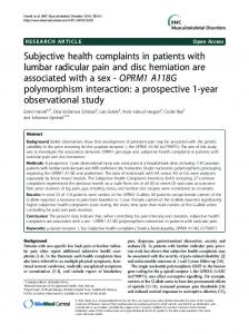
There is an insurmountable flora of possible poles. Analyses using the spatial model therefore reduce it further, stating that opinions tend to correlate: For example that those in favour of universal health care tend to be in favour of high taxes. We then reduce attitudes towards taxes and government spending to a more general socio-economic axis. The multidimensional spatial model usually ends up with 6 - 7 cross cutting axes that represent fundamental social cleavages and which describes all relevant aspects of a given party system. Regulars are center vs. periphery, church vs. state, rural vs. urban and economic class partisanship (Budge 2006; Gallagher, Laver and Mair 2006, p 265-72). The unidimensional spatial model however, states that all relevant political issues can be represented by one axis alone, illustrated in figure 2.1. While two parties may differ in how much they disagree on different subjects, the relevant information can be summarized by one super axis. Ever since the French revolutionaries divided themselves at the king’s left and right hand in the constitutional assembly, this has become the label of this most important division of political opinions.

Figure 2.1: The Unidimensional Left - Right Axis for party “Circle” and party “Square”. This thesis could have been expanded to a multidimensional spatial model, covering several of the political axes. Restrained by resources, I have chosen to restrict it to the most parsimonious. So what is the left - right division? Empirical investigations suggests that it differs. In one of the latest and most thorough investigations by Benoit and Laver (2006, p. 191-212), left-right positions can be well predicted based on socio-economic issues and questions of moral lifestyle, such as gay rights and abortion rules. But several scholars suggests a

2.1. THE SPATIAL MODEL

7

movement towards “new politics”, where the traditional questions of economy must recede to post-materialist issues such as environmentalism and anti-authoritarianism (Inglehart 1977; 1990). There also seems to be differences between the old Western and the new Eastern democracies, where nationalism is much more important in the latter. This is in line with investigations done by Huber and Inglehart (1995). As the authors note, the left-right dimension “can be found almost wherever political parties exist, but it is an amorphous vessel whose meaning varies in systematic ways with the underlying political and economic conditions in a given society.” (Huber and Inglehart, 1995, p. 77). Noberto Bobbio provides a label that may capture the most important aspect across all these subjects. In his classic “Left and Right. The Significance of a Political Distinction” (1996, p. 60), it is argued that the criterion most used to define left and right is attitude towards equality. This label may summarize what matters across different cleavages, such as economic, religious or geographical equality. But the debate of the content is not, and might never be, finished. A correct placement of parties along one or more axes is important because we believe it affects several aspects of society. Theories state that they can tell us about election results, government formations, political stability, policies and policy outcomes and maybe even the most important social conflicts in a given society. In extension we believe this has relevant effects on the everyday life of individuals, in areas like development, liberty and economy. The literature has a wide flora of empirical implications of left-right positions (see for example Brady and Leicht 2008; Gehlbach 2013; Strøm, M¨ uller and Bergman 2008). Given the ambiguousness of the content of the dimension, it is unclear if a left-right position score of, for example, 2 has the same implications across party systems and through time. Most right-wing parties of western Europe does not identify themselves – and they are seldom identified by others – with right-wing parties of eastern Europe, even though they might be scored quite equally on left-right measures. Ideological range is therefore an often used measure, as opposed to the substantial position. The idea is that a difference score between two parties of, for example, 5 implies the same amount of conflict across systems. If this is true, then it does not matter what they are arguing about, as long as we capture the degree of ideological conflict. Due to the strict assumption in the validation method employed in this thesis, all replicated models correspond to this latter usage of the left-right measure. Parties’ actual positions on the left-right scale is unobservable. This is the fundamental challenge when evaluating policy position. Again, to cite Benoit and Laver (2006, p. 141), “[i]t is very difficult, and perhaps in a strict epistemological sense it may be impossible, to demonstrate that a given measure of some fundamentally unobservable concept is more valid than some alternative measure.” We can observe how parties regard different policies, but we can not observe how this aligns in our spatial model. It must be theoretically constructed, and empirically evaluated. The latter is the aim of validation.

8

2.2


Validity, Reliability and Construct Validation

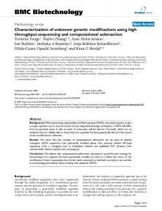
To measure is to develop one or more observable indicators for a theoretically defined concept and give scores or categories to the units in question based on these indicators. The main issue is the relationship between the concept (party position) and the indicators to measure this (different left-right sources). “Valid measurement is achieved when scores [...] meaningfully capture the ideas contained in the corresponding concept.” (Adcock and Collier, 2001, p. 530). This is best understood as the movement between four levels, from the most abstract to the most concrete. Adcock and Collier’s (2001, p. 531) framework is adopted in figure 2.2 to illustrate the measurement levels for the spatial model.

Figure 2.2: Measurement Levels of the Spatial Model Level 1 is the background concept. It is the most broad understanding of a phenomenon, which in this case is the concept of political ideology. Level 2 is the systematized concept. It is an explicit definition of the concept. The unidimensional spatial model of party ideology is such a systematized concept. Level 3 are the definitions of the indicators. These are often referred to as the operationalizations. In general, there are three indicators in the literature: Experts, voters and party manifestos, discussed further in part 2.3. Level 4 are the actual scores given to each party. This thesis discusses the relation between levels 2 - 4, and excludes the broader understanding of ideology. This is what Adcock and Collier (2001, p. 533) defines as measurement validity: How well do you measure what you wish to measure? High validity is understood as low systematic error in how the concept is measured. Reliability, on the other hand, concerns the random measurement error. Low reliability does not cause systematic bias in a measure, but causes a random error which increases uncertainty on the true value: Repeated application of a procedure with low reliability yields unequal values (Adcock and Collier, 2001, p. 531). As will be explained in section 2.3, there are several sources of uncertainty that cause such random error in the measurement of party positions.

2.2. VALIDITY, RELIABILITY AND CONSTRUCT VALIDATION

2.2.1

9

Validation Strategies

There are at least three main strategies for validating measures: content-, convergentand construct validation. Content validation asks whether or not the indicators we use to measure a concept includes all relevant components of that concept, and excludes all irrelevant components. While this is often a theoretical endeavour, it is sometimes associated with factor analysis. The second strategy is convergent validation (Adcock and Collier 2001; Bakker et al. 2012, p. 9; Gabel and Huber 2000; König et al. 2013, p. 14). In this strategy, measures are validated if they show high correlation with other measures of the same concept, and low correlation with measures of other concepts (Adcock and Collier, 2001, p. 540). It is the most common procedure in the literature. This thesis, however, will apply construct validation: In a domain of research in which a given causal hypothesis is reasonably well established, we ask: Is this hypothesis again confirmed when the cases are scored (level 4) with the proposed indicator (level 3) for a systematized concept (level 2) that is one of the variables in the hypothesis? Confirmation is treated as evidence for validity. Adcock and Collier 2001, p. 542

The main assumption made in such validation is that a certain causal hypothesis is true, hence the label given by Adcock and Collier (2001, p. 542): “AHEM: Assume the Hypothesis, Evaluate the Measure”. Convergent validation has a similar assumption, only it assumes that some other measure is “true”. For example: H1) Party manifestos is the place where parties give a true representation of their policy position, while experts often confuse preferences with the actual behaviour they are designed to explain. Or H2) Experts can give a thorough evaluation of a party’s position from several sources, while manifestos alone only give a crude simplex coding. Since “neither measurement claims nor causal claims are inherently more epistemologically true”, the two assumptions are juxtaposed (Adcock and Collier, 2001, p. 543). Objections. There are three main objections to applying construct validation (Adcock and Collier, 2001, p. 543). First, it is argued that there may not exist any hypothesis that can reasonably be assumed to be true. But we can not predetermine such statements about reality, and there are several causal hypotheses that we have more reason to believe to be true than the measurement hypotheses within this literature – for example that parties who disagree more cooperate less easily (Martin and Vanberg, 2003, p. 325). I argue in part 4.1 that the assembly confidence literature provides several such hypotheses. Second, construct validation will lead to circularity. A measure that have been validated by a certain causal hypothesis, can not subsequently be used to test and confirm the same hypothesis. Therefore, construct validation can not become standard procedure. However, as a once-in-a-while analysis, it will hardly pose a threat. Last, construct validation assumes not only a certain causal claim, but also that the other variables involved are valid measurements of their respective systematized concept.

10


In the assembly confidence literature, most other measures are unambiguous. The main conclusion should be that when conducting construct validation, one must carefully choose causal hypotheses 1) that are intuitive, 2) where the other measures involved are unproblematic and 3) where the respective measure have a strong explanatory power. In other words, the causal hypotheses should be a “most likely case” for the measure: If the measure can’t make it here, then it can’t make it anywhere (Gerring, 2007, p. 91-93). I argue that the assembly confidence literature is such a case. I return to this in part 4.1. While the complications are ample, so are the benefits. By testing how the measures perform in “natural environments”, the test provides informative answers to questions scholars are wondering about when they are choosing measures for their own tests. Convergent validation allows us to evaluate similarity per se, but construct validation allows us to evaluate similarity in ways that matters to everyday regressions.

2.3

Measuring Party Position

When assessing party position, we conclude about an unobservable party position based on evidence from an observable source. The literature has three main sources: 1) Party Manifestos 2) Experts and 3) Mass surveys of voters (Castles and Mair 1984; Huber and Inglehart 1995; Budge, Klingemann, Volkens, Bara and Tanenbaum 2001; Ray 1999). In later years, a distinction has arrived between traditional human coded party manifestos, and computer automated content analysis of party manifestos (Laver, Benoit and Garry 2003; Slapin and Proksch 2008). In this section, I give a general overview of these sources, the discussion surrounding their validity and reliability, and the measures included in this thesis and how they were created. An overview of the included measures and their source is listed in table 2.1. Table 2.1: Overview of the included measures and their sources Manifesto, Computer Wordfish

Manifesto, Human Rile KimFording Vanilla

Expert Judgements CMHIBL CHESS

Mass Surveys ESS EVSWVS Eurobarometer

But before I continue, a comment should be added on exactly what units these measures attempt to position. What is a party? The literature is constantly treating political parties as unitary and often rational actors (Adams, Clark, Ezrow and Glasgow 2006; Baron and Diermeier 2001; Brady and Leicht 2008; Gehlbach 2013; Martin and Stevenson 2001; Martin and Vanberg 2003; 2004; 2005; Strøm et al. 2008). In modern representative parliamentary democracies, the parties are the most important link between governing institutions and the people. Yet parties consists of many pieces, such as members, some of them in party cadres, political advisers, central leadership and government ministers. Ideological disagreement within parties may be equally or more important for the relevant theories, than ideological disagreement between them. In the studies replicated

2.3. MEASURING PARTY POSITION

11

here, the unit in study is the parliamentary part of the parties, e.g. the unitary position of the several human beings of a party that reside in parliament or government (Laver and Schofield, 1990, p. 15-28). An important aspect for the validity of the measures in this test is that they are actually measuring this.

2.3.1

Party Manifesto

Party manifestos is the source with by far the most extensive collected data on parties’ position. Since all political parties in modern democracies communicate their political program in textual format, this source allow for a great coverage. As the only source among the three, party manifestos allows for positioning of older parties as long as their political program can be made available through text. Content analysis of party manifestos rest upon salience theory. The theory states that unobservable attitudes are made observable through communication and can be measured through frequencies. It is assumed that the relative emphasis on a specific policy issue for a given party can be used to reveal a specific policy position. Party strategists try to identify the majority electoral position across different issues. They will try to get ownership of the popular position, and emphasize these preferences. A popular example is taxes. For the most part, parties do not mention taxes if they want them heightened, because this is an unpopular phrase. Instead, they are pro public services. Another party however, might gain ownership to the idea of a slim state, and emphasize the need for lower taxes (Klingemann et al. 2007, p. 116; Laver and Garry 2000, p. 620). If salience theory is wrong, then the positions are wrong. Content analysis consider words or sentences as data points. In extension, the process of generating text can even be considered to be a stochastic process, and thus we can also measure the uncertainty for the positions through advanced resampling methods. Understood as data, longer texts provide more precise estimates than shorter texts (Benoit, Laver and Mikhaylov 2009; Laver et al. 2003; Slapin and Proksch 2008). There are mainly two approaches to coding party positions from such documents: human expert coding and automated computer coding. The most important labour of positioning party manifestos is operated by the Manifesto Research Group/Comparative Manifesto Project (Henceforth, both are abbreviated to CMP) (Volkens, Lehmann, Merz, Regel, Werner, Lacewell and Schultze, 2013). These data have been cited more than 1500 times according to Google Scholar, and become “the only (comparable) means of estimating party left-right positions over a long time period in a large number of countries.” (Gabel and Huber, 2000, p. 95). They use human coders to place each quasisentence in the document in one of 56 policy-issue categories. “A ’quasi-sentence’ is defined as an argument or phrase which is the verbal expression of one idea or meaning” (Klingemann et al., 2007, p. xxiii). The frequency of the total sentences placed within each category is used as a sign for the issue’s salience for the given party. There have been invented several different ways to compute an actual left-right scale from these frequencies. With the rapid innovation of computer science, the dominance of CMP as an easy accessible source for parties’ policy position is being challenged by automated content

12


analysis (Laver and Garry 2000; Slapin and Proksch 2008). These methods also employ word frequencies, but they can be constructed by anyone with a computer using open source software such as Wordscores (Laver et al., 2003) and Wordfish (Slapin and Proksch, 2008). The potential of automated computer coding is huge. Political actors constantly inform others of their political opinions through speech and written text. As long as we have access to speeches, manifestos or other linguistic sources, we may map the position of parties since the very birth of modern democracy. We may position news agencies, twitter accounts, commentators and other actors in the political sphere. As noted by Grimmer and Stewart (2013, p. 1), “[t]he primary problem is volume: there are simply too many political texts” [emphasis in original]. This is the major innovation of automated content analysis compared to human coded text: It provides the means to simplify the vast amount of latent data out there. This is acknowledged by both sides of the camp: To the extent that wholly automated procedures reproduce MRG/CMP ones, we can look forward to them eventually taking over the processing of texts with enormous savings of time and money for coding, and an extension of content analyses from programmes to actual policy outputs (e.g. laws). Klingemann et al. 2007, p. 117. Validity. It might be that parties write their election manifestos in light of future events they know will occur. For example, the conservative and right-wing party of Norway were quite certain that they would be able to build a coalition government following the 2013 elections. This might have influenced how they wrote about the areas they knew would become an issue in the government bargains. In that case, manifestos will be influenced by the phenomenons we want them to explain. In general, however, party manifestos are expected to be quite independent of coming events. It does raise the question: For whom do parties write manifestos?’ They could be populist documents written to gather votes, and then disregarded the day after election day. Alternatively, manifestos could be the authoritative stance of a party, a document they always must defend that they comply with and which is sanctioned by party congresses (Laver and Garry, 2000, p. 620). It has been uncovered that CMP includes not only manifesto documents, but also advertisements, drafts, party magazines and speeches. Gemenis (2012) finds evidence that this causes systematic error in the measurement of parties’ left-right positions. Every left-right measure based on manifestos in this thesis originate from this database. For automated computer coding, developing different schemes is cheap since they do not need to take training of coders into account. Computers however, can not correct unforeseen problems in the coding process like a human, or the different meanings of a word in different contexts. It could represent the sacrifice of validity on the altar of reliability. Reliability The reliability of computer coded manifestos is assumed to be good since the source is very clear and computers are 100 % reliable to the algorithm. But they


13

are dependent upon two initial manifestos that define the extreme ends of the left-right axis and which it ’trains’ the algorithm. It is not obvious that different training data will yield similar results. One of the major objections against the CMP data is that they underrepresent uncertainty in at least two ways. First, only one coder codes each manifesto. Different coders on the same document could yield different scores, which would uncover uncertainty (Benoit and Laver, 2007, p. 130). CMP argue that such reliability issues are mitigated through strict definitions, extensive training and central control (Budge and Pennings, 2007, p. 138). It should be safe to say that we have no clue to what degree this mitigates the problem. Second, the CMP data are based on only one coding scheme, invented in the early 1980s, of the theoretically several possible schemes (Laver et al., 2003, p. 311,312). There is reason to believe that a scheme created today would look different. Using several would make the measures more robust, but the high costs associated with developing such schemes, training coders and gathering data have prevented anyone from trying (Benoit and Laver 2007, p. 130; Slapin and Proksch 2008, p. 707). In addition, most computations based on the CMP data assume that the sentence-categories that are relevant for the left-right axis are all equally relevant, which may or may not be true. In addition, they often assume that the importance does not vary through time (Slapin and Proksch, 2008, p. 706,707,711). CMP data tend to be more volatile than other measures. For example, Fianna Fail in Ireland had two manifestos in 1982. One of them is coded -8, the other -32 on CMPs left-right score (Rile, see below), indicating quite a policy jump for this party in a relative short time period. It is so far impossible to know whether this is because the measure is better at mapping ideological movement, or because it is more uncertain (Benoit and Laver, 2007, p. 131). Automated content analysis suffers from no such reliability errors. However, whether they are coded by humans or computers, party manifestos may have significantly different usage in different countries. There is a general uncertainty for their comparability across countries and through time. Party Manifesto Measures Wordfish Wordfish is one of the methods in automated computer coding of party manifestos, developed by Slapin and Proksch (2008). A shortcoming is that there is no complete data set for modern democracies. But because of the uncontested accessibility of this measure, I was able to produce the necessary data. The main goal of Wordfish is to create an easy-to-implement method of measuring party position without requiring expert knowledge on the party system at hand (Slapin and Proksch, 2008, p. 719-20). With Wordfish, the position of a party at a given election is given by the frequency of different words in their manifesto. Different words, however, have different impact upon the positioning. To find this, the script needs two initial manifestos assumed (by the researcher) to be at the extreme ends of the left-right scale, which trains the algorithm. Wordfish is an unsupervised method, which means that the analyst does not impose

14


any word categories on the script, and there is no definition of the left-right dimension. Instead, using discriminant analysis on word frequencies, the software identifies how important different words are in differing between the manifestos. Based on the initial two manifestos, word usage is assumed to belong to different left-right positions. It is up to the researcher to feed the program text that seems meaningful to belong to some left-right dimension (Slapin and Proksch, 2008, p. 408-10). Formally, the functional form of Wordfish is as follows: yijt ∼ P oisson(λijt )

(2.1)

λijt = exp(αit + φj + βj ∗ ωit )

(2.2)

where y is the count of word j in party i’s manifesto at time t. α is a set of party-election year fixed effect and φ is a set of word fixed effects. β is a word specific weight that tries to capture how important word j is in discriminating between party positions where ω is the estimate of party position for a specific manifesto. The word frequencies are assumed to be generated from a Poisson-distribution. This implies the na¨ıve Bayes assumption stating that the probability that a word occurs in the text is independent of the position of the other words in the text. This is most likely wrong, but has been found to be competitive with the more advanced alternative methods relaxing this assumption (Friedman, Geiger and Goldszmidt 1997; McCallum and Nigam 1998, p. 1; Slapin and Proksch 2008, p. 708, 709). For all party systems, I used the following procedure: 1. Download all available party manifestos from the CMP homepage, https://manifestoproject.wzb.eu/ primarily in text format (.txt), otherwise as portable document format (.pdf). 2. Convert any .pdfs to .txt using the software PDF Mate (http://www.pdfmate.com/) 3. Clean the text by making all letters lowercase, remove numbers, punctuation and other symbols that are not words, removing “stop words”, strip unnecessary white space and last stem the words. This was done with the R-package tm (Feinerer, Hornik and Meyer, 2008). The process of removing stop words and stemming the document follows the definitions in this package. 4. All words mentioned in only 10 or less documents are removed. This is recommended by the developers in order to avoid heavy weights for infrequent words (Proksch and Slapin, 2009, p. 7). Changing the exact threshold made very little difference. 5. Identify the potential rightmost and leftmost party-year document by using the CMPs own left-right measure for the manifestos, the Rile-score (see below). If the respective document was missing, I moved on to the second right- and/or leftmost document. Since I do not possess expert knowledge of all party systems, some measure had to be used to identify these. Any of the other measures could have


15

been used. The rationale for choosing the Rile-score is that it is already at party manifesto-level and does not rely on other sources. Rile is a content analysis of the party documents, and the two documents should have dissimilar word usage. This is hopefully better captured by the Rile-score than the expert judgements or mass surveys, where the sources are not necessarily party manifestos. 6. Run the Wordfish script in the R-package Austin (Lowe, 2013). The procedure assumes that word meanings and word usage has been relatively constant, the latter partly mitigated by step 4 (Slapin and Proksch, 2008, p. 711). These assumptions are only expected to give results close enough to the truth. While the construction of this measure is paved with shortcuts, heroic assumptions and loss of control to computer algorithms, it did allow me to position 203 parties between 1958 - 2013 within the time frame of this thesis. A drawback for the data collection is the dependence upon text in a format that is readable by the computer. Certain .pdfs does not allow the computer to identify words, and must therefore be manually written into another format. With serious resources, the data collection could cover more parties and systems and have better authentication of the source texts and the resulting measures. The potential of Wordfish is uncontested. Rile The Rile-score is CMP’s own left-right scale of the human coded party manifestos. The operationalization is straight forward. Some of the categories in CMP are categorized as “left” and others as “right”. The categories were created a priori. Afterwards their fit was investigated through factor analysis. The percentages of sentences falling within these categories are summed up, and then the leftist sum is subtracted from the rightist sum, resulting in a Rile-score between -100 (most leftist) and +100 (most rightist) (Budge et al. 2001, p. 21, 22; Laver and Budge 1992, p. 25 - 30). Table 2.2 gives an overview of the two categories. Since the calculation is based on percentages, sentences that do not belong to any of these categories also affect a party’s position. Imagine two party manifestos, both with 100 left-sentences and 200 right sentences. In the second manifesto, there are also 400 sentences that do not belong to any of these categories. The position score in the first manifesto will be 33.34, and in the second it will be 14.2. The team argues that this makes the measure able to draw “holistic information over all categories” (Budge et al., 2001, p. 23). However, one could equally argue that the measure is sensitive to irrelevant information. At least it implies that irrelevant sentences pushes parties to the center. Since all studies replicated here somehow requires the measures to correctly place relative distance between parties or parties and a median, this center-bias might reduce the Rile-score’s performance. A possible flaw in this measure is that the content of left-right politics may have changed over time, so that this might be a correct definition only for a subset of the relevant periods. KimF. The measure created by Kim and Fording (1998) is very similar to Rile, but will not be affected by sentences outside of the leftist- and rightist-categories. They use

16

CHAPTER 2. PARTY POSITION Table 2.2: Right and left sentence categories, p. 22 in Budge et al. 2001 Right emphases Military: positive Freedom, human rights Constitutionalism: positive Effective authority Free enterprise Economic incentives Protectionism: negative Economic orthodoxy Social Services limitation National way of life: positive Traditional morality: positive Law and order Social harmony

minus

Left emphases Decolonization Military: negative Peace Internationalism: positive Democracy Regulate capitalism Economic planning Protectionism: positive Controlled economy Nationalization Social Services: expansion Education: expansion Labour groups: positive

the same categories, but includes a division in the equation: P osition =

Percentage Leftist Statements - Percentage Rightist Statements Percentage Leftist Statements + Percentage Rightist Statements

(2.3)

This gives a score between -1 and 1, where 1 is most leftist (Kim and Fording, 1998, p. 79). Vanilla. As a way to get a more holistic measure from the CMP data, Gabel and Huber (2000) invented the Vanilla measure. It differs from Rile in that it does not give an a priori definition of the content in the left-right dimension. Instead, the “dimension is defined inductively and empirically as the “super-issue” that most constrains parties’ positions across a broad range of policies” (Gabel and Huber, 2000, p. 96). This is achieved by regression scores from a principal factor analysis to explore what categories correlate to some underlying dimension which they afterwards label as the left-right dimension. They argue that the factor should be made by pooling all countries and years, giving a “global” content of the left-right dimension that applies to all countries at all times (Gabel and Huber, 2000, p. 98 - 100). Such a purely inductive approach to the left-right dimension has been criticized. In constructing a spatial model of political preferences, we have no objective criteria for what is substantially relevant. Benoit and Laver (2006, p. 198) argues that “much of our work has already been done by generations of people who have talked about politics before us”, and all of this is thrown away when we employ a “giant feral factor analysis.” MCSS The Manifesto Common Space Score (MCSS) is an interesting newcomer to the flora of measures, based on Bayesian factor analysis. Its motivation is twofold. First, they question whether the wording of manifestos really is comparable across different party systems and points in time. Second, they find it problematic that the nature of the left-right dimension is defined afterwards by the individual researchers, as with the ’Vanilla’-measure (König et al., 2013, p. 1 - 3).


17

Following Lowe, Benoit, Mikhaylov and Laver (2011), they recode CMP’s data into a logit scale with the formula θ(L) = log(R + .5) − log(L + .5)

(2.4)

where R is the number of right-sentences and L is the number of left-sentences and θ(L) is the logit scale. The + .5 makes small frequency counts more stable without significantly disturbing those with higher numbers. The scale has two important features: First, differences are relative. This implies that going from L = 10 and R = 5, to L = 10 and R = 6 is different from moving from L = 50 and R = 20 to L = 50 and R = 21 (Lowe et al., 2011, p. 131, 132). It does not have “end” points, but extreme positions requires exponentially more sentences. Second, it does not have a natural “center”, such as 0 on ’Rile’. Lowe et al. (2011, p. 125) claims that this approach better satisfies “political, linguistic and psychological criteria” as well as “[exhibiting] superior empirical properties” to the other CMP measures. When categorizing left- and right-sentences, they follow König and Luig (2012). This is summarized in table 2.3, copied from König et al. (2013, p. 5). In addition, the MCSS method attempts to control for country- and time-specific effects, making the measure more comparable across party systems and through time. This is done through two assumptions. First, a parameter for country specific bias is calculated as the difference between position taken in the party’s first time European Parliament (Henceforth: EP) election and the previous national election. They call this the “zero hour” hypothesis: “parties took the same position in their first EP election as in the previous national election” (König et al., 2013, p. 9). The bias is therefore the difference in position between these two elections. Table 2.3: MCSS Left and Right categories, p. 5 in K?nig et al. 2013 Issue Internationalism European Integration National way of life Military Freedom Administration

Enterprise Market Protecitonism Macroeconomics Quality of life Welfare state Traditional morality Multiculturalism Labor groups Target groups

Pole A (Leftist) 109 Internationalism/negative 110 European integration/negative 601 National way of life/positive 105 Military/negative 106 Peace/positive 201 Freedom and human rights/positive 202 Democracy/positive 404 Economic planning/positive 405 412 413 403 406 409 416 501 503 504 604 607 701 705

Corporatism/positive Controlled Economy/positive Nationalization/positive Market regulation/positive Protectionism/positive Keynesian demad management/positive Antigrowth economy/positive Environmental protection/positive Social justice/positive Welfare state expansion/positive Traditional morality/negative Multiculturalism/positive Labor groups/positive Underprivileged minority groups/positive

Pole B (Rightist) 107 Internationalism/positive 108 European integration/positive 602 National way of life/negative 104 Military/positive 605 Law and order/positive 305 Governmental and administrative efficiency/positive 401 Free enterprise/positive 402 407 414 410

Incentive/positive Protectionism/negative Economic orthodoxy/positive Productivity/positive

505 Welfare state limitation/positive 603 Traditional morality/positive 608 Multiculturalism/negative 702 Labor groups/negative 704 Middle class and professional groups/positive

Second, a parameter for time bias is calculated based on the “incentive” hypothesis:

18


The party that gained the largest seat share in an election does not change its position in the next election (König et al., 2013, p. 10,11). Any difference in position between these two is assumed to be bias. By these two hypotheses, they argue that the measure is more comparable. To create an actual scale that is not defined inductively, they use the Chapel Hill Expert Survey Series (Henceforth: CHESS, see below) data to calculate means and variances for each party family. This is set as the intercept and variance for parties that belong to the respective family. The trajectory of the parties is thereafter modelled using polynomials (König et al., 2013, p. 9). A drawback with the MCSS measure is that it is dependent upon CMP for most of the positioning, EMP2 for EP elections and country parameters and CHESS data to define the means for each party family. If we wish to have a measure that can be used for all parliamentary systems and not only those that are members of the EU, as for example Norway, this strategy is simply not viable. In addition, the measure becomes more resource demanding and thus reduces one of the prime advantages of manifesto based measures. This weakness is also its strength. The specification of the “zero hour” and “incentive” hypotheses makes the comparability assumptions explicit and tries to handle it. None of the other CMP measures does this, even though they are constantly used with the implicit assumption that they can be compared across party systems and through time.

2.3.2

Expert judgements

An intuitive strategy to get valid measures of party positions is by asking people that somehow are experts on the respective party systems. In such studies, party systems are coded by several experts. The mean value is employed as the party’s position and standard error as a measure of uncertainty. Asking several experts is expected to increase the precision, and is used by all expert survey measures included in this thesis. Experts can use various sources, including manifestos, parliamentary voting behaviour, public appearances etc. They will often know all relevant parties within a party system and are not dependent upon available manifestos. Without doubt, the combined works of the many experts in such surveys have been key for the rise of this tradition within political science. Still, the measure is not without its flaws. Validity A common issue with expert surveys is the inability to go back in time to measure past party positions. Using today’s experts to judge older party systems might reduce the expert-knowledge, biasing the scores towards modern perceptions (Slapin and Proksch, 2008, p. 706). Experts might have an ambiguous relationship which sources they use when giving scores to parties. For example, the position of the Dutch “Freedom Party” might be based solely on the position of the eccentric party leader Geert Wilders. If so, it might 2

The EMP data are equal to the CMP data for EP elections, with the same categories (W¨ ust and Volkens, 2003).


19

fail to capture a unitary stance of the whole parliamentary group. The source might vary from party to party, and it is unclear if experts should change their main source for positioning the party (Budge, 2000, p. 103-04). Changing sources opens up for the possibility that experts are coding based on the phenomenons the measure is supposed to explain. For example, in the autumn 2013 in Norway, the conservative party “Right” went for the first time into a minority coalition with the most right-wing party “Progress Party”, who never before had been in government. This could affect how we perceive the position of these parties. But if these parties in the future are said to have moved closer, it is unknown if this is because they actually changed policy positions, or if they entered in a coalition. What we want, is to measure the former phenomenon in order to explain the latter phenomenon – not the other way around. Reliability Expert judgements suffer from both intra- and inter-coder reliability issues (Slapin and Proksch, 2008, p. 706). Such problems arise when two different experts, possibly from across countries and over time, understand the questions, sources and range of possible positions differently. Repeated application of the process could yield different values. A way to mitigate this is to have some of the coders to code several party systems, so that the same expert is part of several different “groups” of experts. This could increase the comparability of the measures between groups of experts. In none of the measures included have this been done. There might be a bad incentive structure in expert surveys. In order to be a part of an academic society, one is expected to contribute by – among other things – answer such surveys without receiving compensation. Instead of doing thorough evaluations, all experts might simply be coding a party or party system according to some important work within the field. For example, it might be that all experts simply codes right-wing parties based on the work by Cas Mudde.3 To assign a number to the party is the only thing needed to get the social and academic benefit, while extra investigation steals time from other work. If several experts have the same primary source, this contributes to a fake illusion of certainty: They are not independent measures of a party. In spite of these flaws, expert surveys is the one source that maximizes the possibility that one is asking the most well-informed individuals and gets as much information as possible into the measure at a manageable price. They allow for thorough evaluations of party systems, and are not dependent upon access to one specific type of source. The Expert Survey Measures Castles and Mair The expert judgement data set by Francis Castles and Peter Mair from 1984 has become a classic within the literature and cited in 741 articles according to Google Scholar. It is one of the first real attempts to create a systematic cross-national spatial scale for left-right policy positions for Western Europe, The Unites States and 3

For those who don not know him, he is a famous political scientist studying right-wing parties.

20


the Old Commonwealth. 3 - 17 experts in each country placed parties on an eleven-point scale with the following labels: Ultra-Left (0); Moderate Left (2 12 ); Centre (5); Moderate Right (7 21 ); Ultra-Right (10) (Castles and Mair, 1984, p. 75). There is no definition of the left-right dimension. It is therefore unknown what the different experts have been judging, and whether or not they understand the concept equally. This creates uncertainty about comparability between experts’ scores (Van Deth, 2009, p. 3). Huber and Inglehart John Huber and Ronald Inglehart’s “Expert Interpretations of Party Space and Party Locations in 42 Societies” from 1995 has also become a classic measure within the literature. As a follow-up to the survey by Castles and Mair, it has been cited 799 times. They conducted their analysis in 1993 as one of the first expert surveys since the fall of the Soviet Union. The motivation behind Huber and Inglehart’s survey was to map the political conflict in the eastern Europe, as well as the impact it had on other European party systems (Huber and Inglehart, 1995, p. 73-75). They wanted to map three things. First, they wished to know if the language of the left-right dimension was applicable to these new democracies. Second, they investigated whether or not the unidimensional spatial model of political ideology captured all of the relevant information. Last, they wanted to know how different systems put different substantive meaning into the understanding of these dimensions. The experts where asked to do five things (Huber and Inglehart, 1995, p. 77): 1. Decide if the left-right dimension best described the two major poles of the party system. If not, then write the labels they found most appropriate. 2. Write the name of the parties on a ten-point scale. 3. List the key issues that divide the parties on the main dimension. 4. State whether there existed a second dimension and if so, label it. 5. Place the parties on this second dimension if applicable. Given the results, they found that 10 categories define the left-right scale: Economic conflict, centralization of power, property rights, constitutional reform, xenophobia, national defence, authoritarianism vs. democracy, isolation vs. internationalism, traditional vs. new culture and conservatism vs. change. These measures also had a high correlation (.94) with the (at the time) ten years old measure from Castles and Mair, indicating that this might be how most experts understood the content of the left-right dimension also in that survey. They compared how the answers on question 3 were distributed among these 10 categories in different countries (Huber and Inglehart, 1995, p. 80, 84, 90). While the unidimensional left-right framework was widespread, there were differences in how important the different categories were. Benoit and Laver Kenneth Benoit and Michael Laver conducted an expert survey in 2002 - 2003 for the book “Party Policy in Modern Democracies” (2006) with a thorough discussion of the spatial model of political preferences. In only 8 years the work has attracted 979 citations. As with Huber and Inglehart (1995), they define the left-right


21

dimension inductively. They asked experts explicitly for multidimensional scores. In addition, the experts were asked to place the parties on a “general left-right dimension, taking all aspects of party policy into account” (Benoit and Laver, 2006, p. 192-93). They define the content of the unidimensional left-right scale by its correlation with the others. As with Huber and Inglehart (1995), the content varies between countries (Benoit and Laver, 2006, p. 191-12). Yet they do conclude that unidimensional policy can be predicted based on socio-economic and moral lifestyle (gay rights, abortion etc.) issues. CMHIBL Castles and Mair, Huber and Inglehart and Benoit and Laver are all “snapshots” from a single point in time. However, since the correlation between them is high, I have merged these to create a cross-national time-series data set of party position.4 This new data set (Henceforth: CMHIBL) perform better than any of the three measures separate in the analyses. In order to simplify presentation, only CMHIBL will be utilized. The issue of national comparison of the left-right content in these three expert surveys is probably less critical in this analysis. This is because the replications are all located in the old developed western democracies. Both Huber and Inglehart (1995) and Benoit and Laver (2006) report that in this context, the left-right dimension’s most important characteristic is socio-economic policy. CHESS The Chapel Hill Expert Survey Series (Henceforth: CHESS) has gradually become a dominating measure within the expert survey tradition. It contains a total of 4 waves conducted between 1999 - 2010, recently published in a trend file (Bakker et al. 2012; Hooghe, Bakker, Brigevich, de Vries, Edwards, Marks, Rovny, Steenbergen and Vachudova 2010; Steenbergen and Marks 2007). It is one of the few attempts to build a cross-section time-series data set of party positions based on expert judgements, although it is restricted to the European countries. CHESS asked the respondents to characterize the parties in terms of their broad ideological position on a left-right eleven-point scale. The content of the left-right scale has never been specified, but the wording of the question has been equal for each wave (Bakker et al. 2012, p. 3; Hooghe et al. 2010, p. 700; Steenbergen and Marks 2007, p.353). The main advantage of CHESS is that it offers a cross-national time-series of expert surveys. The stability of the wording makes it possible to compare movement through time. A downside is the lack of any thorough analysis of the content of the left-right scale. As Benoit and Laver (2006, p. 203) note, since content is different between countries, it might also be different between points in time.

2.3.3

Mass surveys

Certain mass surveys ask the respondent to place their own position, and what party they voted for or feel close to. This information can be used to measure parties’ position, 4

This has already been done by D¨ oring and Manow (2012), although they also include the 2010 wave of CHESS.

22


for example by the mean position of all respondents that voted for the respective party (Gabel and Huber, 2000, p. 98). Such a measure of voters’ self-placement and what they voted is a crucial aspect in representative government. Mass surveys are likely to give a better measure of the position of the respective party’s voters. It might also be a good measure for the parliamentary part of a party, if it taps into the incentive structure of the politicians. The analyses replicated in this thesis might be least likely cases for mass surveys, but if they perform well, it could indicate that there is a close relationship between the preferences of parties and their voters. This linkage can not be observed in a clear way elsewhere, which makes these surveys unique in their own respect. Validity Mass surveys rests on the assumption that voters place themselves independently of the party they vote for. If this is not true, then the measure might be coded based on the phenomenons it is supposed to explain. For example, if voters tend to a priori agree with the party they identify with, then the behaviour of the party could be affecting the voters’ position. If a party issues a no-confidence motion against a government party, this could signal ideological distance between the two. If this affects how voters perceive their own position, then the measure is explained by the phenomenons we (in turn) believe the measure can help to explain. This contributes to uncertainty concerning the causal direction in hypothesis testing. None of the included surveys define the content of the left-right dimension. If how respondents understand the dimension differs systematically with other traits, such as social class, education, workforce and so on, the measure of a party’s position will be systematically biased depending on the composition of it’s voting citizens. In addition, it could increase the probability that answers are affected by the latest news, the preceding questions in the survey or other random events. It is impossible to go back in time to correct any mistakes in a given mass survey or acquire measures of past positions. In addition, these surveys are highly costly to conduct. Never have stratified sampling design been used to make sure all relevant parties will be represented among the respondents. The result is low coverage of parties and sometimes an unstable wording of the questions. This makes such measures unsuitable for many research designs (Ray, 1999, p. 285). Reliability. The same inter- and intra-reliability issues apply here as with expert judgements. First, the lack of definition is expected to increase random error. Second, voters may have different perceptions of the relationship between the actual scores on the scales: The distance between 0 - 1 on a ten-point scale might be perceived unequal to the distance between 5 - 6, and this might vary between respondents. While there are possible solutions to this problem, they have not been applied until recently, and never for the surveys included here. A more technical issue with mass surveys is the low quality of their documentation. Some simply use abbreviations for party names even though several parties in a system match the same abbreviation. Others simply refer to the party family, for example “the conservatives”, while there might be more than one party that match this description.


23

This increases the probability of making erroneous merge-links when preparing data, which lowers reliability. The Mass Survey Measures European Social Survey The ESS has been conducted biannually since 2002. In every wave, respondents (15 years and up) have been asked to place themselves on a leftright ten-point scale and what party they voted for. The sampling method varies between countries, but all must adhere to principles of representativeness through probability. My data are created from their trend file of waves 1 - 5 (ESS 2012a; 2012b; ISSC 2014). The data have been weighted with ESS’ design weight. This is their recommended weight when creating means within the countries (ESS, 2007). Eurobarometer The Eurobarometer is the European Commission’s own mass survey, in order to map the public awareness, knowledge and attitudes in the EEC/EU. The first wave was in 1970, and since 1974 the survey has been conducted twice a year. It contains 1000 respondents from all but the least populated countries included. Up to 1989, there were country-specific variation in sampling methods. The data used in this analysis is The Mannheim Eurobarometer Trend File, covering the period 1970 - 2002 (Schmitt and Schloz 2005; ISSC 2014). In several of these waves, the respondents were asked to place their own left-right position on a ten-point scale, where 1 represented most left and 10 most right. In addition, they were asked what party the voted for in the last national election. The long time series and frequency of the waves in Eurobarometer makes it a strong candidate among the mass surveys. European Values Survey and World Values Surveys Four European Values Survey (Henceforth: EVS) waves have been conducted, in 1981, 1990, 1999 and 2008. Sampling methods have varied between the years, and between the countries involved. Methods for data gathering have also varied, from hired interviewing agencies in 1981 to trained face-to-face interviewers in 2008 (EVS 2011;ISSC 2014). In every survey, they asked the respondent to place themselves on a ten-point leftright scale. In 1981, they asked which party the respondent felt close to. In 1990 and 1999, they asked what party the respondent would vote for if there was a general election today. If the respondent was unsure, then they would ask what party appealed the most. In 2008, they first asked if the respondent would vote and if yes, then what party. If no, they would ask what party appealed the most. Due to the instability both in data collection and wording of the question, there is reason to expect a low reliability, which could disturb the true measurement of parties’ placement. There have been five waves of the World Values Surveys (Henceforth: WVS) between 1981 - 2008. The sixth wave has been executed but is not yet ready. Each country specifies their own sampling design, but these must be approved by the WVS Executive Committee. Kittilson (2007, p. 871) mentions that in “most countries, survey teams

24


employ a form of stratified multi-stage random probability sampling. However, in remote areas where this proves difficult, survey teams may employ cluster or quota sampling”. Exact sampling design varies between the waves, creating uncertainty for comparability of the measures (ISSC 2014; WVS 2009). In every survey since 1990, the respondents have been asked to place themselves on a left-right ten-point scale, as well as what party they would vote for if there was a general election today. If the respondent is uncertain, they would be asked what party appealed to them the most. EVS and WVS are very similar. For example, the waves in 1981 - 1984 and 1989 - 1993 are equal, with EVS being responsible for the European countries. Since then, they have conducted separate waves but with quite equal questionnaires. They provide instructions for how to combine the two data sets. In the analysis, there was no significant difference between EVS alone and EVS merged with WVS.5 To ease presentation, only the combined measure will be utilized.

2.4

The Contemporary Issue

The literature validating party position measures suffers from at least two shortcomings. First, unless more diverse validation strategies are employed, the literature will be stuck in a situation where measures are true because a lot of different measures agree: A truth through consensus. Second, as scientists we need more information than current comparisons yield. I will start with the first claim. So far, the most common analysis within this literature is to show that the measure has a high or low correlation with other measures. Yet measures that are not theoretically motivated, such as the Vanilla measure (Gabel and Huber, 2000, p. 95), correlate with those that are theoretically motivated. It remains unsettled what this implies for the measures that are theoretically motivated. Furthermore, scholars disagree on what measure should be the “golden standard” with which all else should correlate. Jonathan B. Slapin and Sven-Oliver Proksch concludes that While [expert] surveys often come up short as pooled cross-sectional time-series data, they do provide researchers with a method for checking the validity of position estimates from other methods in addition to providing a snapshot of party positions at one point in time. Slapin and Proksch 2008, p. 706.

This is supported by Gabel and Huber (2000, p. 98). Ian Budge on the other hand, argues that expert judgements confuse preferences with the actual behaviour they are designed to explain, and are ambiguous about the time period involved, the criteria used to locate parties and what exactly they are locating. Budge 2001, p. 211. 5

WVS alone lacks several of the European parties, making it unsuitable to use alone.

2.4. THE CONTEMPORARY ISSUE

25

Dinas and Gemenis (2009, p. 1,2) agree with Budge in that manifestos “provide more accurate and representative picture of where the parties stand in the policy space, without requiring further knowledge about their policy record.” Over the years, measures have been used to do “mutual” validations over time. For example, every wave of CHESS has been validated by showing correlation with CMP and Eurobarometer. In 2012 their trend file was released (Bakker et al., 2012, p. 11,12), and again this correlation was demonstrated. However, if every wave correlated with the CMP data, there would be something odd if the trend file of the same waves did not correlate. In 2007, Klingemann et al. (2007, p. 63 -84) compared the standard CMP ’Rile’-score to Castles and Mair (1984), even though this had been done seven years earlier by Gabel and Huber (2000). The methodological fallacy in repeating the same correlations as validity tests is equivalent to choosing dependent units (selection bias): They are not independent tests of the the hypothesis that source X is a good operationalization of the systematized concept (King, Keohane and Verba, 1994, p. 124-25). Eventually, we run the risk that all measures will have indirectly or directly been shown to correlate with most other measures in the literature, and we run out of possible tests. Recent publications have found creative new ways to test validity. For example, Lowe and Benoit (2013) recognized that a computer based coding of political texts should be as similar as possible to how a voter would code the same text, and ran a comparison between these two. Any deviation is a sign of “wrongness” in the measurement. Such creative diversion of validation strategies is exactly what the literature needs. The second and more important claim is that we need more informed comparisons. A simple correlation does not inform us of the quality of these measures, because “alternative indicators of a systematized concept may be strongly correlated and yet perform very differently when employed in causal assessment” (Adcock and Collier, 2001, p. 542). While the correlation between measures is an interesting aspect, we should be equally interested in how they correlate with everything else. For example, Matthew Gabel and John Huber (2000, p. 102) concludes that CMP data, when using the Vanilla method to place party positions, “can be used to obtain reasonably accurate predictions of parties’ left-right placements.” This conclusion is based on several regressions showing a correlation with different expert judgements and mass surveys. But how accurate is reasonably accurate? Vanilla got a significant intercept of -4.89, significant beta of 1.54 and a mean absolute deviation (MAD) of 0.69 in a bivariate ordinary least squares (Henceforth: OLS) regression, while the measure from Klingemann, Hofferbert and Budge (1995) only got respectively 2.15, 1.15 and 0.98 in a similar regression (Gabel and Huber, 2000, p. 99). But what are the implications for social inquiry? The interpretations of correlations seem to be in the eye of the beholder. Recently the MCSS measure based on CMP was released, and its validity was confirmed by showing higher correlation with CHESS than the other CMP measures – Vanilla and Rile. It was concluded that MCSS “differ substantially from alternative measures derived from the manifesto data but are more in line with expert survey data” (König et al., 2013, p. 16). This conclusion was drawn the year after the CHESS trend file, based on correlations with the CMP data, had concluded that “[o]verall, the analyses suggest relatively high

26


levels of common structure across the different measures.” (Bakker et al., 2012, p. 11). There seems to be no standard for “high”, “low”, “good” or “bad” correlation. The result is that we are presented with estimates of correlations, but it does not inform us of anything when we want to recommend one measure over the other. This is why a construct validation is in order. A tool that can predict real world observable phenomenons is a better representation of reality than a tool that fails to do so. By comparing which measure is best at predicting the social phenomenons that our theories suggests that these measures should be able to predict, we get an informed comparison of the different measures’ utility for social inquiry. It does not provide any final answer, but it will aid scholars when they need to choose measures for hypothesis testing.

Chapter 3 Research Design If I give you my data, isn’t there a chance that you will find out that I’m wrong and tell everyone? Yes. Gary King

In this chapter I will do three things.1 First, I aim to explain how the different leftright measures were merged with the replication data. Second, I defend that listwise deletion is the correct response to missing data in this analysis, even though imputation is to be recommended in most other statistical analyses. Last, I defend that the main analysis used in this thesis, the K-fold cross validation method, is a simple yet powerful test of models’ predictive power.

3.1

Data

This thesis is made possible by the “Parliament and Government composition database” (Henceforth: ParlGov) from Döring and Manow (2012). It is a large documentation of the traits of different party systems since 1945, and earlier for some countries. It includes all parties (1400), elections (680) and governments (960) for 38 countries. It maps how parties change party names, which helps to avoid coding errors due to insignificant name changes. It includes party IDs for many of the different left-right measures used in this analysis, information on which parties sat in government, and which were in opposition. The three replicated articles all provide their replication data, but only Williams (2011) includes identification of the parties to the corresponding left-right measure. The two other include the point in time which the relevant phenomenon in the dependent variable took place. I used ParlGov to identify the party systems at this point in time. New cabinets are defined in line with the rest of the literature as 1

Chapter quote from Gary King’s “Replication, Replication” 1995, p. 451

27

28

CHAPTER 3. RESEARCH DESIGN (I) any change in the set of parties holding cabinet membership; (II) any change in the identity of the prime minister; (III) any general election; (IV) any substantively meaningful resignation. Döring and Manow 2012.

For each party, I then merged the party with each of the data sets containing the various left-right measures. For each party at the different points in time, I use the temporally most proximate measurement.2 The relevant merge IDs are provided by ParlGov for the manifesto and expert survey based measures in this thesis. For the mass-surveys, I created the IDs. The ParlGov homepage provides thorough information on party changes, different names and links to other data sets (Döring and Manow, 2012). In cases where the mass-survey documentation only provided abbreviations which could match several of the parties in a system, the necessary information (election results, name changes, history e.g.) was usually available. If I could not be certain about which party ID would be correct after investigating, the party was coded as missing. The database use a conservative definition for parties and keep the same ID for splitting parties. This is different from for example the CMP data, where parties are coded at the election level. Since ParlGov provides the necessary merge keys, this does not pose an issue (Holger Döring, personal correspondence). When creating ranges or medians for the different replications, the measures are required to have no missing observations. For example, when creating the range within government for the replication of Martin and Vanberg (2003), the range is unknown if the position of any of the government parties is unknown. The same goes for the median parliamentary position for the replication of Williams (2011).

3.1.1

Missing

Missing values occurs when a measure do not have any measurements of a party. The best response to missing values in time-series cross-section data is to use a multiple imputation model and exchange missing cells with predicted values (see for example Honaker and King 2010). However, this is not viable in this setting. If I “invented” party positions for all missing parties, it would be hard to evaluate the quality of the different measuring methods. The performance of a measure with low coverage could become more dependent upon on the imputation method instead of the measuring method. In this analysis, there is no other solution than listwise deletion, despite its flaws. The assumption for listwise deletion is that missing values are generated completely at random. This is certainly not true. Missing data tend to cluster in time. Newer leftright measures lack old parties that are no longer existing, and vice-versa. In addition, missing cluster by country when whole party systems are not covered by a measure. Listwise deletion will cause biased standard errors (Honaker and King, 2010, p. 564). Even though it is the right thing to do in this evaluation, imputation would be a better strategy when the measures are used for standard hypothesis testing. 2

I tested with different interpolations, but the results differed very little.

3.2. K-FOLD CROSS-VALIDATION

29

Missing values is a real issue in a world with resource constraints, something any analyst must take it into account when choosing data. Whether the result of a measuring method is a crude measure or a low coverage does not matter; both are equally useless for causal assessment. As the next chapter will show, missing data is a more important source for error than the measurement methods. Therefore, missing data is a relevant aspect of the different measures, and should be a part of their evaluation.

3.2

K-fold Cross-Validation

The K-fold cross-validation (Henceforth: K-fold CV) is the main analytical method used in this thesis. It is a method that aims to investigate the out-of-sample predictive power of a regression model (James et al., 2013, p. 181-86). The basic idea is simple: Divide the data set into k “folds” (parts), with no observations overlapping. Use k-1 folds to estimate the regression coefficients, and use these to predict the dependent variable in the excluded fold. Repeat this process k -times, so that all folds have been predicted by combination of the others. This is illustrated in figure 3.1. 5−Fold CV

Figure 3.1: The 5-fold cross-validation method. The regression is repeated five times, excluding different folds of the data indicated in yellow. The response in the excluded part is predicted by the coefficients from the included parts, marked in blue. Figure is copied from James et al. 2013, p. 181 To summarize the predictive power of the model, it is typical to show some sort of error between the true and the predicted outcomes. In this analysis, I use the mean square root of the squared error (Henceforth: MRSE), which is the the mean absolute distance between the predicted outcome and the true outcome. Formally, it is found by n q 1X M RSE = (yi − fˆ(xi ))2 (3.1) n i=1 where fˆ(xi ) is the predicted outcome for the ith observation, and yi is the true outcome. Small MRSE indicates better predictions (James et al., 2013, p. 29,30). The method enables researchers to investigate how sensitive the model is to different samples. The MRSEs within the different folds can uncover how the predictive power is

30

CHAPTER 3. RESEARCH DESIGN

dependent upon certain samples of data. The method can also produce a straightforward comparable summary of the quality of the various models by averaging the MRSE for each individual fold – often referred to as the “K-fold CV-estimate”.3 The K-fold CV procedure can also be used for binomial outcomes, as in Franchino and Høyland (2009), but with the number of misclassified observations instead of MRSE as a measure of model power. Since the different measures differ in their number of observations, I add a second step to the analysis, where all data sets are reduced to the data set with the lowest coverage. This is to minimize the impact of different observations. I do this by sampling this many observations 100 times from the data sets of the 10 alternative measures. The K-fold CV analysis is repeated on all 100 samples of each of the measures. If the data were simply reduced to the size of the smallest data set, the results could be affected by which sample was drawn. By repeating the process 100 times, the analysis avoids that any of the measures suffers from an “unlucky” draw. For example, the model from Martin and Vanberg (2003) investigates government bargaining durations. Some cases are harder to predict, as for example the Dutch general election in 1977, in which it took 205 days to negotiate a government – 178 days longer than the mean duration in the data set. An unlucky draw would be a draw that includes a series of hard cases, resulting in a higher MRSE. A measure that lacks several of the hard cases however, will never experience this and thus benefit from low coverage. This is avoided by repeating the process 100 times. By the same logic, I use the most “lucky” draw – the lowest “5-fold CV-estimate” – of the 100 samples to compare the results achieved across the 100 samples. Since the distribution of mean MRSEs across the 100 draws will be affected by the content of the complete data set it is drawn from, the most lucky draw ensures a higher equivalence in the comparisons, and avoids punishing a measure for an accidentally unlucky sample. Alternatively, a comparison between the most “unlucky” draws could have been carried out to indicate which measure avoids the least precise results. However, missing observations is more prominent for parties and systems that are atypical. Measures like ESS and CHESS have lower coverage because they focus on the typical representative democracies in Europe. The measures from manifestos and EVSWVS, on the other hand, expands the scope with more deviating cases which are harder to predict. The most “unlucky” draw is more influenced by the distribution of missing data than the most lucky draw. The most lucky draw is therefore a superior comparison of measurement validity. For the models in Martin and Vanberg (2003) and Franchino and Høyland (2009), which use left-right range within government, I remove all one-party governments from each fold when they are predicted. In one-party governments, all measures have a range of 0. Comparing these cases will therefore make the results between measures appear more equal. When reducing the data sets 100 times, I therefore sample so that each data set have an equal number of one-party and multi-party government observations. In this thesis, I have chosen to use 5 folds. In theory, one may choose any number of 3

Given by CV(k) =

1 k

k P i=1

M RSEi .

3.2. K-FOLD CROSS-VALIDATION

31

folds, for example k = n, where each individual observation is predicted by all the others. This is an inferior strategy because it would cause severe computational problems. For example, in the K-fold CV analysis of Franchino and Høyland (2009), the data will be reduced to 3777 observations. This is done 100 times for 11 different measures. Choosing k = n would result in over 4 million regressions.4 Choosing five folds greatly reduce the computational time. In addition, it has been shown that reducing the number of folds only have minor impact on the prediction bias (James et al., 2013, p. 183-84). To summarize, I will first execute the 5-fold CV analysis on each measure as they are. Then I repeat this 100 times for each measure with reduced data sets. This gives a robust comparison of the predictive power of the models without the need for dramatic computational resources. The strategy is fit to maximize the equivalence between the measures’ data sets so that the different results are caused by different measurement methods of the left-right position. Doing both steps, and by comparing the MRSE within folds, this design allows for investigation of the importance of different data content. This is the best available strategy for the construct validation employed here.

4

4154700 = (11 · 3777) · 100

32

CHAPTER 3. RESEARCH DESIGN

Chapter 4 The Original Articles Parliamentary democracy is the world’s most popular political project. Kaare Strøm

In this chapter I will go through the three models replicated in this thesis, each in three steps: First, I explain the relevant theory for the explanatory left-right variable. Second, I show that the original model can be replicated correctly. Third, I illustrate the descriptive statistics for the alternative left-right measures, and replicate the model using these. With each model, I illustrate the effect of the relevant variable with simulated predicted values (Brambor, Clark and Golder, 2006, p. 73,74). Before I get into the individual articles, I give a general overview of the assembly confidence literature, and why this was a suitable area to look for theories to replicate.1 The main message from the chapter is that insignificant results due to lack of data is a much bigger issue than measuring wrongly. The tests should only be considered as preliminary, since the replications differ in the number of observations. This will be solved with the 5-fold CV analysis in chapter 5.

4.1

Assembly Confidence: A Most Likely Case

The assembly confidence literature revolves around parliamentary democracies, and how and when parties will choose to cooperate in legislation. Specifically, it deals with the relationship between cabinet and parliament. The main actors are political parties and politicians. The scene of the play is the national assemblies, and the hypotheses are manifold: Political careers, passing of bills, political parleys, coalition life-cycle etc. There are three reasons for why this is an optimal case for evaluating party policy positions. First, ideological party position is central in most of the associated theories (Gehlbach 2013; Strøm et al. 2008). 1

Chapter quote is from Kaare Strøm’s “Delegation and accountability in parliamentary democracies”, 2000, p. 1

33

34

CHAPTER 4. THE ORIGINAL ARTICLES

Second, the theories are highly developed. Studying the behaviour of political parties in parliament is a political science-speciality, and dates back (at least) to Hotelling’s “Stability in Competition” from 1929. Today, this has evolved into a sophisticated theoretical framework that covers several empirical implications (see for example Strøm et al. 2008; Gehlbach 2013). Last, there is good data coverage, and many of the associated variables are unambiguous. One of the possibles ditches for construct validation is low validity of other variables in the causal hypothesis. In the assembly confidence literature, most variables are straightforward, such as parties in parliament, seat share, minority cabinet, cabinet duration etc. Arguably, the most ambiguous of the recurring variables is party ideology (Chiba, Martin and Stevenson, 2014, p. 2). I will replicate three models from the assembly confidence literature in order to test the predictive power of the party position measures. These are well established studies with quality (and available) data. They are gathered from different phases of a cabinet life-cycle: duration of government bargaining, cabinet monitoring and vote of confidence.2 The three models require different scope and precision from the measures, summarized in table 4.1. The replications differ in temporal and geographical scope, the scope of national parties it is expected to measure, and at what precision the measure will be tested. All of the models use some sort of ideological range, either between a subset of Table 4.1: Overview of Replicated Theories Period Country Level Precision

Bargaining 1950 - 1990 10 european countries Government Range

Monitoring 1979 - 2004 15 EU member states Government + Support Range

NCM 1960 - 2008 20 countries Opposition Dist. from median

the parliamentary parties or from the median position. In the following, I explain the three theories in sequence, present their descriptive statistics and replicate them using the different left-right measures. These replications should be considered as preliminary tests. They may inform us of whether or not different measures would yield substantially different conclusions, but because of differences in data coverage, these replications can not conclude on the quality of the measurement methods.

4.2

Government Bargaining: Martin and Vanberg

In “Wasting Time? The Impact of Ideology and Size on Delay in Coalition Formation” Martin and Vanberg (2003) argue that ideological discrepancy between parties makes coalition negotiations more difficult, resulting in longer bargaining duration. The connection between these two phenomenons is so tight that Grofman and van Roozendaal (1994, p. 159) used bargaining duration as a measure for political disagreement. 2

Two models of government formation were also prepared, but the replication material were too poor.

4.2. GOVERNMENT BARGAINING: MARTIN AND VANBERG

35

There are at least three theories for why ideological disparity should delay government formation negotiations (Martin and Vanberg, 2003, p. 325-26). First, when party leaders decide to enter coalitions, they must have the implicit support of the party members. Party “leaders [...] are not the only decision makers whose preferences are central to successful coalition bargaining.” (Martin and Vanberg, 2003, p. 325). It becomes harder for leaders to anticipate what coalitions will be acceptable to the veto players of one’s own and others’ parties as ideological distance between them grows. Ideologically proximate parties are more likely to have cooperated in parliament before and thus be more familiar with each other’s party dynamics. Furthermore, ideological distance may imply more constituencies with larger variations, making it unfamiliar what sort of political pressure the party leadership must deal with. “In short, there are strong reasons to suppose that party leaders will be better able to judge which kinds of proposals are acceptable to parties that are ideologically close to their own” (Martin and Vanberg, 2003, p. 325). Party ideology may also matter because greater distance imply smaller ’winset’ - a smaller set of policies that a sufficient majority of the parties will agree to. Thus a more detailed agreement may be necessary in order to convince all coalition partners. Last, delaying negotiations may be a way for parties to signal perseverance and loyalty to campaign promises or election programmes. Such signals becomes increasingly important as ideological range grows because large compromises are unavoidable. Delays may be a way to signal voters that the party leaders worked as hard as they could.

4.2.1

Original Method and Replication

Martin and Vanberg (2003) estimate a Cox proportional hazards model in order to investigate how different covariates affect the duration of government bargaining. Their data consist of 203 governments from 10 countries between 1950 - 1993. 225 units are included in the original data set, but the original authors lacked left-right range measures for 22 of these. The Cox model is one of the “event history”-models, and more specifically a type of duration-model.3 The results from a Cox-model are “hazard ratios“: The probability that a unit will “end” at this time, given that it has “survived” (or lasted) until now (Steffensmeier and Jones, 2004, p. 2,3,14,50). In duration models, the dependent variable is the duration (for example number of days) before the event occurred. Such models avoid unrealistic assumptions and wrong predictions that a linear model like OLS would produce. Since the duration can not take a negative value, assuming linearity could predict (impossible) negative durations. The coefficients would be both inefficient, inconsistent and biased (Long, 1997, p. 217,218). The original results are correctly replicated in table 4.2.4 These results are equal to model 3 on page 330 in the original article. The interesting covariate is “Range of government”, coded as the absolute range between parties, using Vanilla as the left3

More popular called “survival” models The original formula had countries coded as their first letters. This caused erroneous variance estimators because Ireland and Italy and Norway and Netherlands were clustered as similar countries. The mistake is replicated in table 4.2, but correcting it does not alter the substantial results. 4

36


right measure. As this shows, increased ideological disagreement increases the bargaining duration significantly at the conventional 5 %-level. Descriptive statistics for the rest of the variables are available in appendix A. Table 4.2: Replication of Martin and Vanberg, 2003 Covariates Post-Election Previous Defeat Continuation Identifiability Range of Government Number of Government Parties Number of Government Parties * ln(T) Minority Government

Beta -0.56 (0.17) -0.12 (0.23) 1.15 (0.24) 0.14 (0.12) -0.24 (0.12) 1.37 (0.13) -0.49 (0.04) -0.47 (0.21)

Log-Likelihood -722 N 203 Notes: The original table can be found on page 330 in the article. Standard errors in parentheses

4.2.2

Replication with other left-right measures

The distributions and descriptive statistics of ideological range using the alternative leftright measures is available in figure 4.1. The large frequency of zeroes across all measures are caused by one-party governments. Other than that, the distribution differs slightly, some being more right-skewed than others. Pairwise Pearson-correlations are illustrated in figure 4.2. Besides from the original left-right variable from Martin and Vanberg (2003), Wordfish correlates the least with the other variables. Their original analysis use the Vanilla-measure from Gabel and Huber (2000). The correlation between their measure and my own Vanilla measure is 78, which is the highest correlation for the original variable. At least three things could cause a difference in these two. First, some of the government parties might not have been identified perfectly. This can happen if they have noted different parties in government at a given time than ParlGov (Döring and Manow, 2012). Their replication data makes it impossible to investigate this further. It could also be caused by different interpolation methods, and different software when doing the factor analysis. As will be shown, this is not a serious issue. When replicating the model with the different measures, I employ the Weibull-model


0

20

40

60

0.0

0.5

1.0

1.5

60

100

Min = 0, Median = 1.93, Mean = 1.97, sd = 1.89, Max = 8.17

0 20

60

100


0 20

60

100


0 20

0 20

60

100

Min = 0, Median = 11.87, Mean = 15.82, sd = 17.21, Max = 70

37

0.0

0.4

0.8

1.2

0

2

4

6

8



Min = 0, Median = 0, Mean = 0.75, sd = 0.97, Max = 4.2


0

1

2

3

4

60 0 20

60 0 20

60 0 20

60 0 20 0 1 2 3 4 5

100

MCSS

100

Vanilla

100

KimF

100

Rile

0

1

2

3

4




1.0

2.0

ESS

3.0

2

3

4

Eurobar

60 0 20

60 0 20

60 0 20 0.0

1

100

EVSWVS

100

CHESS

100

CMHIBL

0

0.0

1.0

2.0

WORDFISH

3.0

0.0

1.5

3.0

Original

Figure 4.1: Descriptives of “Range of Government”, Martin and Vanberg 2003 instead of the Cox model. This is because the Cox model is unfit for prediction, since it does not specify the baseline hazard, and therefore provides no intercept: It tells us how covariates affect duration, but it is impossible to calculate expected duration lengths. The Weibull-model is a possible alternative which makes this possible. It specifies the hazard rate as monotonically decreasing or increasing, which fits well with the data (Steffensmeier and Jones, 2004, p. 21,22,25-31,48-49). Changing to the Weibull-model does not alter the substantial conclusions. A comparison is provided in appendix A. In the main analysis in chapter 5, I also remove the interaction between the number of coalition parties and the logarithm of bargaining duration, since the latter term is partly what the models will try to predict. The interaction was originally included to avoid violating the proportional hazard assumptions, that all covariates have an equal effect on the duration at all time points. I specify the Weibull model as an accelerated failure time model so that this will not be an issue (Steffensmeier and Jones, 2004, p. 24-27).


W O R

D FI

SH

38

Eu r

ob

ar

100

WORDFISH

55

100

EVSWVS

56

93

100

CMHIBL

65

82

89

100

ESS

69

88

94

90

100

MCSS

59

81

82

77

93

100

CHESS

62

75

87

93

88

87

100

Vanilla

55

70

72

74

77

72

80

100

KimF

55

65

71

76

79

72

80

83

100

Original

45

58

67

62

76

72

72

78

74

100

Rile

50

61

68

73

76

70

80

81

95

74

R

ile

O

rig

in a

l

Ki

m

F

Va n

illa

C

H

ES

S

M

C SS

ES S

C M

H IB L

EV SW

VS

Eurobar

−1

−0.8

−0.6

−0.4

−0.2

0

0.2

0.4

0.6

100

0.8

1

Figure 4.2: Correlation between “Range of Government”-variables, Martin and Vanberg 2003 The effect of “Range of government” points in the same direction for all the 11 leftright measures. This is shown in figure 4.3. This figure shows the simulated effect of this covariate across 11 models. The simulated effect is found by drawing 1000 samples from the multivariate normal distribution, using the coefficients (β) as mean and variance equal to the variance-covariance matrix of the model. This process gives more precise uncertainty for the effect of ideological range, conditional on the value of the other covariates (King, Tomz and Wittenberg, 2000, p. 349-50). All figures show predicted values of bargaining duration (Y-axis) over the range of values of the left-right range (X-axis) for a two-party majority government in a country without continuation rule and all numeric variables at the median value at the first day of bargaining. The black line is the point-estimate, and the red shaded area indicate the 95 % confidence intervals. Considering the point estimates, most of the measures indicate a total increase of about 5 bargaining days if the level of ideological range moves from its minimum value to its maximum value. Vanilla and CMHIBL have a stronger effect within their full range. If we consider the significance, only KimFording, Vanilla, MCSS and CMHIBL achieve


39

Simulated Predicted Values of Left − Right Range Across 11 Models

5

5 1.0 2.0 Original 203

3.0

Barg. Days

15 10 5

20

40 Rile 192

20 15 10

2

4 6 MCSS 172

8

Barg. Days

20 15 10 5

20 15 10 5

0

1 2 3 EVSWVS 139

4

10

0.0

20 15 10

1.0 2.0 WORDFISH 185

15

0.4 0.8 KimF 192

5 0.0

20

5 0.0

5 0

10

60

0.4 0.8 Vanilla 192

20 15 10 5

0 1 2 3 4 5 CMHIBL 175

Barg. Days

Barg. Days

20

15

5 0

Barg. Days

0.0

Barg. Days

10

Barg. Days

10

15

20

Barg. Days

15

20

Barg. Days

Barg. Days

Barg. Days

20

0

1 2 3 CHESS 113

4

20 15 10 5

0.0

1.0 2.0 Eurobar 163

3.0

0.0

1.0 ESS 103

2.0

Figure 4.3: Simulated predicted values of “Range of Government”, Martin and Vanberg 2003. X-axis is the range of the “Range of Government”-covariate. Y-axis is the predicted number of bargaining days. 95 % confidence intervals in shaded red. significance on the conventional 5 %-level.5 Furthermore, several measures do not guarantee a different predicted value at its minimum value compared to its maximum value. This should not be given much importance in this test. The different measures differ in their coverage. Using ESS instead of the original measure would have halved the number of observations. In addition, the models differs in which observations are included. Some observations might be more important than others for the estimates. For example, Wordfish has 185 observations and MCSS 172. But as can be seen in figure 4.1, Wordfish 5

Some of the others turn significant at certain non-linear specifications.

40


has a higher frequency of one-party governments among its observations, giving shorter ideological ranges. This makes it harder to efficiently estimate higher values. Establishing equivalent data sets is the task of chapter 5. In this replication, the similarity of the patterns is more interesting. First, if any of the measures were not able to tap the left-right dimension, the patterns should give more counter-intuitive results. Neither does. Second, the figure tells us nothing of which measure provides the most correct estimates. We do not know the true magnitude of the effect of ideological disagreement. This as well will be better evaluated in chapter 5, when the predictive power of the models will be put to the test. Therefore, the main message from the replication of Martin and Vanberg (2003), is that some measures would not provide the necessary data, but all measures would indicate the same pattern: Ideological range between bargaining parties increase the duration of the bargains. The result supports the notion that none of the left-right measures give counter-intuitive results.

4.3

Coalition Monitoring: Franchino and Høyland

In coalition governments, there is a danger that individual ministers will diverge from the coalition agreement for individual gain – a classic principal-agent problem. This is possible because “parties have complete autonomy over the ministries they control” (Gehlbach, 2013, p. 88). Among other things, ministers enjoy an information advantage over their jurisdiction, and norms of ministerial responsibility discourages interference from other cabinet ministers. Since political preferences between coalition partners diverge, ministers may exploit their position to implement policies in favour of their own party at the expense of other coalition members. However, all members would prefer a negotiated compromise to such ministerial drift (Thies, 2001, p. 584). To enforce such compromises, behaviour must be monitored. The greater the ideological disparity in cabinet, the greater the need to monitor (Franchino and Høyland 2009; Gallagher et al. 2006, p. 43; Martin and Vanberg 2004, 2005; Verzichelli 2008, p. 237). There are different monitoring mechanism parties may use, as for example policy documents or junior ministers as ’watchdogs’ within jurisdiction (Martin and Vanberg 2004; Verzichelli 2008, p. 259). In “Legislative Involvement in Parliamentary Systems: Opportunities, Conflict, and Institutional Constraints” from 2009, Franchino and Høyland argue that the parliament can be used as such a mechanism. Legislatures in modern democracies are “equipped with strong standing committees with broad informationgathering tools capable of neutralizing the information advantage enjoyed by a minister” (Franchino and Høyland, 2009, p. 609). Their study is within the context of the EU, where they argue that the information advantage is especially evident. This is because the minister may, in various ways, have been involved in the process at the EU-level. Implementing the directive is the responsibility of the respective minister. Some directives leave little room for national manoeuvring, but for those that do, the need for coalition partners to monitor behaviour is important. However, the benefit from intervening must be evaluated against its costs.

4.3. COALITION MONITORING: FRANCHINO AND HØYLAND

41

As ideological divergence between partners grows, both the benefits and temptation of ministerial drift and the cost for the victim increases, making parliamentary intervention more worthwhile. And thus Franchino and Høyland (2009) finds evidence that parliamentary involvement in transposition is more common the greater ideological range within cabinet.

4.3.1


The analysis from Franchino and Høyland (2009) utilize a multilevel probit model with random intercept to investigate when the parliament is involved in the transposition of EU legislation. The second level in the model is the different legislations from the EU, which is similar for the EU-nations. The probit model for binary outcomes is a way to model phenomenons with a latent value from −∞ to ∞, but where we can only observe two outcomes (Long, 1997, p. 40, 41). For example, the latent distribution can be the probability for being in the labour force: Two people can both be in the labour force, but with unequal probability. Parliamentary involvement, the binary dependent variable in Franchino and Høyland (2009, p. 610-14), follows an underlying interval variable with a normal cumulative distribution. The multilevel structure was motivated by the fact that observations were not independent. The directives explained a significant proportion of the variance in the probability of parliamentary involvement (Franchino and Høyland, 2009, p. 415). Ignoring the multilevel structure would yield incorrect small standard errors and therefore increase the possibility of a Type 1-error (Steenbergen and Jones, 2002, p. 219-20). I have successfully replicated model 2 on page 616 in the original article in table 4.3 (Franchino and Høyland, 2009, p. 616).6 The important variable is “Conflict”, which appears in no less than 7 interactions. It is coded as the range between the party of the responsible minister, to the most extreme governing or supporting party, using the left-right variable from Ray-Marks-Steenbergen, the precursor for CHESS (Ray 1999; Steenbergen and Marks 2007). We see that ceteris paribus, increased ideological range increase the probability for parliamentary involvement, and this is statistically significant on the 5 %-level. Descriptive statistics for the various variables are available in appendix B.

4.3.2

Replication with other left-right measures.

In recreating the “Conflict”-variable, I could not completely replicate the process adopted by Franchino and Høyland (2009). In the original measure, they use the range from the party of the minister responsible for the transposition, to the most distant coalition partner. For minority governments, they use the range between the government party and the most distant supporting party. These data were acquired from European Journal of Political Research (EJPR), M¨ uller and Strøm (2000) and Woldendorp, Keman and Budge (2011). Where data was not available, they assumed that the closest party was the supporting party. 6

Without robust standard errors for countries. This does not affect the substantial results.

42

CHAPTER 4. THE ORIGINAL ARTICLES Table 4.3: Replication of Franchino and Høyland, 2009 Parameters Intercept Conflict Council Complexity Deadline Years Agenda Control Amendment Prerogatives Confidence Vote Bicameralism Cabinet Turnover Environment Finance Industry Interior Public administration Public Health Social affairs Transport Conflict

Variance, Intercept Log-Likelihood

X X X X X X X

Council Complexity Deadline length Agenda control Amendment prerogatives Confidence Vote Bicameralism

Beta

S.E.

-2.47 5.453 0.282 0.118 0.233 -0.51 0.32 -0.05 -0.057 -0.015 0.419 1.553 0.53 1.575 1.317 0.94 0.704 0.091 2.126 -0.516 0.151 -0.767 -1.676 -0.632 0.333

0.305 1.388 0.121 0.089 0.056 0.201 0.053 0.045 0.046 0.005 0.151 0.208 0.109 0.381 0.388 0.49 0.23 0.14 0.498 0.345 0.223 0.916 0.269 0.205 0.23

0.566

0.752 -1813.207

Notes: The original table can be found on page 616 in the article. Dependent variable is parliamentary involvement. Level 1 N = 6089, Level 2 N = 724

Easy accessible data from these sources is not available, neither for portfolio allocation nor supporting parties. Gathering the relevant data is therefore not possible within the time-frame of writing this master thesis. Instead, I utilize the range within the coalition. For minority governments, I utilize the range between the government and the most distant party needed to achieve 50 % of the seats in parliament. Descriptive information of the different measures is presented in figure 4.4, and the correlation between them in figure 4.5.7 In all measures there is a tendency in the direction of right-skewness, and a large number of zeroes caused by one-party governments. Pairwise Pearson’s correlations are reported in figure 4.5. As should be expected, the original variable used by Franchino and Høyland (2009) correlates the most with its successor CHESS. The lowest correlation, 36, is between the original and ESS. There are large differences between the number of observations across the models. 7

To ease presentation, Vanilla, KimFording and the original measure were multiplied by 10.

4.3. COALITION MONITORING: FRANCHINO AND HØYLAND

0

20

40

60

0

4

8

12

1000

2000


0

1000

2000


0

1000

2000


0

0

1000

2000


43

0

2

4

6

8

0

2

4

6

8





4

8

12

0

2

4

6

1000 0

1000 0

1000 0

1000 0 0

2000

MCSS

2000

Vanilla

2000

KimF

2000

Rile

0 1 2 3 4 5

0




ESS

6

Eurobar

1000 0

1000 0

1000 0 0 1 2 3 4 5

4

2000

EVSWVS

2000

CHESS

2000

CMHIBL

2

0 1 2 3 4 5 WORDFISH

0

2

4

6

Original

Figure 4.4: Descriptives for “Conflict” measures, Franchino and Høyland 2009 Wordfish, with the lowest coverage, only have 3950 of the original 6089 observations. But also CHESS, Eurobarometer, ESS and EVSWVS have less than 5000 observations. This causes several of the parameters to become more uncertain. I show only one simulated effect from the results, which is typical for the model as a whole. The standard result tables are available in appendix B, but are for the most part uninformative as they only show the effect and standard error for the variables when all other constitutive terms in the interactions are equal to zero (Brambor et al., 2006, p. 73,74). Simulated effects are needed to show the effect across the whole scale of the ”Conflict” variable conditional on the value of the other variables (King et al., 2000, p. 349-50). To show the effect of all 7 interactions across 11 measures would take up to much space. The main message is that the three interactions that are significant in the original analysis; council, amendment prerogatives and confidence vote, all have the same pattern across all models, but the significance is lost in several of the models. Here, I illustrate only the interaction with council involvement.


ES S

44

C

M

H

IB L

100

ESS

67

100

Eurobar

77

74

100

EVSWVS

85

75

89

100

MCSS

72

64

77

78

100

CHESS

69

78

81

86

79

100

WORDFISH

58

49

52

65

67

64

100

KimF

59

61

73

78

66

75

61

100

Vanilla

58

58

72

76

71

75

57

85

100

Rile

55

59

71

79

66

77

62

96

87

100

Original

36

53

54

57

54

82

53

59

65

61

O

rig

in

al

R ile

Va n

illa

Ki

m

F

W O

R D

FI S

H

C H ES S

M

C

SS

EV SW VS

Eu

ro

ba

r

CMHIBL

−1

−0.8

−0.6

−0.4

−0.2

0

0.2

0.4

0.6

100

0.8

1

Figure 4.5: Correlation between “Conflict”-variables, Franchino and Høyland 2009 This is done in figure 4.6. The simulations are made as if all numeric variables were at their median value. The solid line with red confidence interval is a simulation where the directive comes from the EU commission. The dashed line with green confidence intervals is a simulation where the directive is from the EU council. The authors note that a “striking aspect is [...] that the effect is substantially much weaker for Commission than for Council directives” (Franchino and Høyland, 2009, p. 615). This conclusion is repeatedly confirmed across most measures. The exceptions are EVSWVS, CMHIBL and Eurobarometer. These models do indicate a stronger effect of ideological range when directives are issued by the council, but it is not significantly different from the effect under commission-directives. ESS and Wordfish confirms the effect, but fails to distinguish the two at higher levels of ideological conflict where coverage is lower. To summarize, the probit model from Franchino and Høyland (2009) is demanding, and lower data coverage impedes estimation. Since the models differ in their observations, the results do not establish the needed equivalence to conclude that differences are caused by different measurement methods. Yet all measures do seem to indicate a pattern in line with theory: Increased ideological distance increases the probability that parliament

4.4. NO-CONFIDENCE MOTIONS: WILLIAMS

45

0.8 0.0

0.4

Pr(Y=1 | Data)

4 6 8 Vanilla N=5582, N Groups=722

0.0

0.4

0.8

2

0

2 4 6 MCSS N=5582, N Groups=722

0.0

0.4

0.8

0 1 2 3 4 5 Eurobar N=4801, N Groups=716

Pr(Y=1 | Data)

0

Pr(Y=1 | Data)

0.8 0.0

0.4

0.8 0.8 0.0

0.4

0.8 0.4 0.0

0.8 4 8 12 KimF N=5582, N Groups=722

0 2 4 6 8 CMHIBL N=5510, N Groups=722

Pr(Y=1 | Data)

0 1 2 3 4 5 EVSWVS N=4657, N Groups=715

0 1 2 3 4 5 ESS N=4705, N Groups=716

0.4 0.0 0

0.0

0.4

0.8 0.4

20

Pr(Y=1 | Data)

40 60 Rile N=5582, N Groups=722

Pr(Y=1 | Data)

0

0.0

Pr(Y=1 | Data)

0 1 2 3 4 5 Original N=6089, N Groups=724

Pr(Y=1 | Data)

Pr(Y=1 | Data)

0.8 0.0

0.4

Pr(Y=1 | Data)

0.8 0.4 0.0

Pr(Y=1 | Data)

Simulated Predicted Values of Left − Right Range Across 11 Models

0 1 2 3 4 5 CHESS N=4892, N Groups=716

0 1 2 3 4 5 WORDFISH N=3950, N Groups=709

Figure 4.6: Simulated predicted values of “Conflict”, Franchino and Høyland 2009. X-axis is the range of the “Conflict”-variable. Y-axis is the predicted probability for parliamentary involvement. Shaded areas indicate 95 % confidence intervals. Commission-directives in solid and red, Council-directives in dashed and green. will be used for monitoring. This effect is conditional on several other variables. None of the measures contradicts this theory.

4.4

No-Confidence motions: Williams

Only 5 % of all no-confidence motions (henceforth: NCMs) result in government termination. This is the starting point in Laron K. Williams’ “Unsuccessful Success? Failed

46


No-Confidence Motions, Competence Signals, and Electoral Support” from 2011. His goal is to rationalize why parties still choose to issue NCMs. A key assumption is that voters hold leaders accountable for policy performance. Voters do not have full information over performance nor what it is reasonable to hold the different political actors accountable for. Several “contingency dilemmas” distorts information. A NCM allows the opposition to name and shame a particular policy as bad performance. As such, NCM is a tool for opposition parties to “influence the electorate’s perception of the opposition party’s ability to govern relative to the current government.” (Williams, 2011, p. 1480). This is supported by the media coverage that accompanies such events. Thus, NCMs are not about the short-term benefit of removing the government, but a long-term investment in votes. There is a credibility cost involved for the opposition. For the signal to be effective, the opposition party must appear as a credible alternative. Otherwise, it may just as well be perceived as political “cheap talk”. Moderate parties are more likely to occupy the median position. Since any ideologically continuous majority coalition must include the median position, this puts moderate parties in a better bargaining position (Gehlbach, 2013, p. 1 - 22). Parties in the center are therefore more credible alternatives. Williams (2011) show that the further from the median the opposition party is, the less benefit the party gains from issuing NCMs.

4.4.1


Williams estimate four different OLS regressions to estimate how NCMs affect election results. The fourth of these models estimates change in votes for opposition parties, which is the dependent variable. The interesting explanatory variable is ideological extremism, coded as the absolute distance between a party’s position on Rile and 0. Extremism appears in interaction terms with both the number of NCMs against the government and number of NCMs against the government by the given party (Williams, 2011, p. 1489). Descriptives for the variables are available in the appendix C. OLS is the most basic of regression models. It is linear, meaning that one scalar point change in the independent variable changes the dependent variable by β, irrespective of the current level of the dependent variable (Long, 1997, p. 3-5). The model is correctly replicated in table 4.4. The original model can be found on page 1489 in the original article. It should be noted that Williams’ significant tests are one-tailed (Williams, 2011, p. 1489). Statistically significant results at the conventional 5 %-level are therefore achieved if the beta divided by the standard error is equal to or larger than +/- 1.645, as with a significance test at the 10 %-level. The interaction term with the number of party NCMs achieves about -1.8, and would have failed a standard two-tailed hypothesis test.


47

Table 4.4: Replication of Laron K. Williams, 2011 Independent Variable

Beta

S.E.

Constant No. of NCMs agains govt. No. of NCMs by that party Real GDP per capita growth Majority govt. No. of govt. parties Lagged vote share

0.588 -0.198 0.717 -0.128 0.65 -0.046 0.013

0.302 0.081 0.309 0.053 0.263 0.092 0.009

Ideological extremism Extremism x Govt. NCMs Extremism x Party NCMs

-0.006 0.004 -0.02

0.009 0.002 0.011

N Adj. R Squared

693 0.022

Notes: Robust Standard Errors clustered by country to control for heteroscedasticity. Significance tests in the original article are one-tailed

4.4.2

Replication with other left-right measures

Since not all the measures have a natural center, I changed the operationalization of the extremism variable to be the distance from the median percentage. Specifically, I duplicated each party’s row by the rounded number of percentage votes they got each election. For each election, I extract the median position of all parties in that election – the position of the median percentage. Extremism is measured as the absolute distance from this median. This operationalization is in line with Williams’ (2011, p. 1493) theory that “[m]oderate parties are in a better bargaining position because they typically occupy the median position in the system and are therefore featured in more coalition alternatives” (my emphasis). In addition, the ParlGov-database does not include Israel. The country must therefore be omitted from the replication since the necessary IDs needed to merge the different leftright measures are unavailable. The distribution and descriptive statistics of these variables are illustrated in figure 4.7.8 By comparing the original variable and Rile, we see that my operationalization allows for more extreme parties. By definition, most parties lie closest to the median position percentage. More intriguing are the pairwise Pearson’s correlations, illustrated in figure 4.8. Wordfish does not correlate at all with the original extremism variable. In general, correlations between the measures are lower for this analysis than in the preceding replications. The most similar measures are those from mass-surveys. Even Vanilla and Rile only achieves a correlation of .66. It is possible that the low correlations are due to the intermediate step of creating a median, magnifying the dissimilarities for each step: If the measures only correlate 8

Vanilla has been multiplied by 10 to improve presentation

48


60


0

40

80

120

150 0

50

Frequency

150

Frequency

0

50

150 0

20

0.0

1.0

2.0

0

2

4

6

8

Vanilla





2

4

6

8

0 1 2 3 4 5

0

0

Frequency

Frequency

300 200 0

100

Frequency

60 20 0

10 20 30 40

KimF

20 40 60 80

Rile

100

Original

0

0

4

8

12

WORD

CMHIBL




0 1 2 3 4 5 CHESS

0 1 2 3 4 5 EVSWVS

30 20

Frequency

0

10

40 0

0

20

40

Frequency

60

60

MCSS

20

Frequency

50

Frequency

100 150 50 0

Frequency


250


0

Frequency


0

2

4

Eurobar

6

0 1 2 3 4 5 ESS

Figure 4.7: Descriptives for Extremism, Williams 2011 moderately in the first place, then the medians are likely to correlate only moderately. The distance between the position and the median then might amplify the original discord. The results from the different replications can be seen in figure 4.9. The simulations are set as if during a majority, one-party government, and the rest of the variables at their mean values. The solid line with red shaded 95 % confidence intervals is the simulated predicted values over the range of extremism for a party that have issued no NCMs, and no NCMs have been issued against the government in the period. The dashed line with green confidence intervals is the predicted values over the range of extremism, for a party that have issued 3 NCMs against the government, and these are all the NCMs issued against that government in the period. The most striking observation is the uncertainty in the model. When reported with 95 % confidence intervals, the effect in the original model also loses its significance. The predicted value for a median party whom have issued 3 NCMs may be as low as -2.5 % change in support. Had the party been as extreme as possible, the predicted value could

49

O r ig in

al


100 R ile

Original

49

100

KimF

37

93

100

Vanilla

37

66

65

100

MCSS

29

47

51

57

100

CHESS

34

47

50

54

63

100

ESS

21

56

57

51

65

81

100

EVSWVS

28

52

53

44

63

78

89

100

CMHIBL

20

35

37

38

61

66

55

59

100

Eurobar

23

46

48

46

66

82

92

86

52

100

0

1

2

4

9

1

8

15

6

12

−0.4

−0.2

0

0.2

W O

R

D FI

SH

Eu

ro

ba

r

C

M

H

IB

L

EV

SW

VS

ES

S

C H ES S

M

C

SS

Va n

illa

Ki m

F

Rile

WORDFISH

−1

−0.8

−0.6

0.4

0.6

100

0.8

1

Figure 4.8: Correlation Between Extremism, Williams 2011 still have been +2.5% change in votes. Between the models, differences in certainty seems first and foremost to be a result of the number of observations. When looking at the point estimates, most of the models indicate the correct result: the more extreme the party, the less it pays off in votes to issue NCMs. Moving from the least to the most extreme position reduces the expected change in votes by about 2.5 %. This however, is not the result from CHESS, EVSWVS and Eurobarometer, where being extreme is a good thing the more NCMs you have issued. However, this should not be taken as empirical proof against the quality of their measurement methods, as these data contain less than half of the original data set. Wordfish is no different than the others: the point-estimate indicate the correct pattern, but the confidence intervals makes it hard to evaluate if this is statistically significant, as the data with Wordfish only have 68 % of the original data. But automated computer coding certainly does not stand out as especially bad. Again, due to differences in observations, the equivalence needed to determine how the measurement methods affect the results is not achieved. But if one wish to replicate the results from Williams (2011), one needs first and foremost a measure with abundant data.

50

CHAPTER 4. THE ORIGINAL ARTICLES Simulated Predicted Values of Left − Right Range Across 11 Models Robust Standard Errors

0 −5 −10

−5

40 80 Rile N=615

0 −5 −10

5 0 −5

1 2 3 4 WORDFISH N=435

0 −5 −10

10 5 0 −5 −10

0 1 2 3 4 5 Eurobar N=228

5 0 −5

8

0

2

4 6 MCSS N=381

8

0

1 2 3 EVSWVS N=260

4

15

5 0 −5

10 5 0 −5 −10

15 Vote Change

Vote Change

5

4 6 Vanilla N=615

0 1 2 3 4 5 CHESS N=219

15

10

2

10

4 8 12 CMHIBL N=402

10

−10

−10 0

15

−5

15

10

−10 0

0

0

Vote Change

Vote Change

5

5

0.4 0.8 KimF N=615

15

10

10

−10 0.0

15 Vote Change

0 −10

0

Vote Change

5

15 Vote Change

5

15

10

Vote Change

10

Vote Change

15 Vote Change

Vote Change

15

10 5 0 −5 −10

0

1

2 3 ESS N=150

4

0

20 40 60 80 Original N=640

Figure 4.9: Simulated predicted values of “Extremism”, Williams 2011. X-axis is the range of the “Extremism”-variable. Y-axis is the predicted change in votes. Shaded areas indicate 95 % confidence intervals. Simulation with 0 NCMs in solid and red, simulation with 3 NCMs in dashed and green.

4.5

Summary of Preliminary Results

The three articles have been replicated with all the alternative measures, and the simulated effects have been illustrated. There are two relevant patterns across all three models. First, no measure systematically contradicts the tested theories or the other measures. This suggests that they all tap the same underlying phenomenon. Second, if one is looking to get results that are significant at the conventional 5 %-level,

4.5. SUMMARY OF PRELIMINARY RESULTS

51

one should first and foremost choose a measure that maximizes the number of observations. In this respect, the sources differ. Expert judgements and mass surveys will never be able to go back in time to get older measures. The hand-coded manifesto measures may all go back in time as long as the necessary text are available. But the cheapest method would be to use automated computer codes, here represented by Wordfish. The evidence so far does not tell us anything about which measure gives the most precise results, since we do not know which effect magnitude is most ”correct”. Neither have they established the necessary equivalence needed to conclude on the quality of the measurement methods. This is the goal of the next chapter, where the measures will be reduced to equal size, and their predictive power will be used as a benchmark for measurement quality.

52


Chapter 5 Prediction results Only predictive models are scientific. Philip A. Schrodt

In this chapter, I undertake two steps on each of the three replicated models.1 First, I do a 5-fold CV analysis on the data sets of each of the 10 alternative measures, plus the original. Second, I reduce the data sets to the size of the smallest data set through listwise deletion of randomly selected observations and then run the 5-fold CV analysis. This is repeated 100 times in order to avoid especially unlucky samples: Since different data set sizes also imply different content, for example different party systems, outliers or other traits that affect their “representativeness”, doing listwise deletion only once could make a measure randomly end up with a composition of observations that is harder to predict, resulting in higher MRSE than other samples of the observations. This will also be illustrated in the following sections. Repeating the process 100 times allows each measure to show its best side. Comparing the results for both the full and reduced data sets also allows for an evaluation of how important data content is for predictive power. The results will be presented with my interpretations.

5.1

Bargaining Duration

In the bargaining model from Martin and Vanberg (2003), the dependent variable was the duration of government bargains measured in days. When no adjustments are made to the data sets, there are noticeable differences in predictive power. In figure 5.1, the y-axis indicate the MRSE and the coloured marks note the mean MRSE for the five folds – the 5-fold CV-estimate. The measures are aligned along the x-axis, ordered by the number of valid predictions, which is noted in parentheses. The size of the mark is scaled as the number of predicted observations as a share of the full data set and multiplied by 5. Since one-party governments are removed from the predictions, these numbers do 1

Chapter quote from Philip A. Schrodt’s “Seven Deadly Sins of Contemporary Quantitative Political Science”, 2014, p. 291

53

54

CHAPTER 5. PREDICTION RESULTS

not correspond to the data set size. Circles, squares and diamonds indicate respectively manifesto-, expert or mass survey based measures. The grey vertical lines ranges from the minimum to the maximum MRSE of the individual folds for each measure.

35

−

33 31

−

29 27 25

MRSE

23 21 19

− − − − ● ● ● ●

− − ●

17 15 13 11

− ●

− −

− − − − − − − − − −

9

−

7 5 Original (131)

Rile (127)

KimF (127)

Vanilla (127)

MCSS (121)

WORD (120)

CMHIBL (114)

Eurobar (98)

EVSWVS (74)

CHESS (70)

ESS (50)

Figure 5.1: MRSE in the full data sets, Martin and Vanberg 2003. The Y-axis is the MRSE. The x-axis indicate the different measures, ordered by the number of valid predictions. Circles, squares and diamonds indicate respectively manifesto-, expert or mass survey based measures. The coloured mark is the 5-fold CV estimate, and the size of the mark is scaled as the number of predicted observations as a share of the full data set multiplied by 5. The colors are ment to ease comparison of the results. The number of predicted observations is noted in parentheses. The grey vertical lines range from the minimum to the maximum MRSE of the individual folds for each measure. Looking at the sources, we see that all mass surveys, EVSWVS, Eurobarometer and ESS, performs the best, while the difference between manifestos and expert surveys are only minor, missing by 18 - 19 days on average. Wordfish has the fourth best results, and better than its hand-coded siblings. Notice that CMHIBL gets the highest mean MRSE, and had the largest magnitude in the simulated effects in the replication; a stronger magnitude is not necessarily more correct. Rile, KimFording and Vanilla have the same observations and are therefore equivalent in all respects. The only difference between these three is the measure. This figure is therefore an informative comparison of these three measures. Of the three, Rile performs best, and Vanilla worst. As we shall see, this difference is probably coincidental for this analysis.

5.1. BARGAINING DURATION

55

There is a certain tendency that measures with fewer observations perform better, but CHESS and CMHIBL contradict this trend. EVSWVS gets the lowest mean MRSE, more than a day lower than the second place ESS. Eurobarometer is not far behind, and have have 48 more predicted observations than ESS. It is not only the sheer size of n that matters, but also its content and the measuring methods. In general, the original authors could have increased their predictive power by three days by changing to EVSWVS. Nonetheless, it would also imply that 57 observations could not be predicted at all. Furthermore, if these 57 observations are harder cases to predict, and this is what determines the difference in MRSE, then changing measure would not increase prediction power, only reduce prediction possibilities. Data content does account for much of the differences. Looking at the vertical lines indicating the range of the MRSE across the 5 folds, there are clearly large differences depending on the composition of observations within each fold. This is especially prominent for analyses with fewer observations in total. The maximum MRSE value of ESS is five times the size of the minimum MRSE. ESS has the least non-missing observations for multi-party governments, with 50 observations. CHESS has the least one-party governments, with 43 observations. To minimize the impact of the data content, I draw 93 valid observations for each of the measures: 50 multi party and 43 one party governments. To avoid “unlucky” or biased samples, this process is repeated 100 times, and the K-fold analysis is done on each sample. The results are illustrated in figure 5.2. 5-fold CV-estimates are noted along the yaxis, and the respective measures along the x-axis. The large coloured marks indicate the most lucky draw, and a horizontal black line is drawn to ease the comparison of between these. The 5-fold CV-estimate from the remaining 99 draws for each measure are indicated as black marks. Eurobarometer now achieves the best results, a lucky draw which on average is one day more precise than the second place, Wordfish. The difference between the worst (ESS) and the best (Eurobarometer) result is quite equal as with the full data; about 5 days. Since ESS and CHESS decided the number of observations, these will naturally have less variation than the others. This goes especially for ESS, which had the lowest number of multi-party governments: The same observations are predicted 100 times, but in different folds and with different observations estimating the coefficients. For the hand coded manifestos Rile, KimFording and Vanilla, the latter now achieves the best result. This performed worst in the full data. As mentioned, these three have identical observations. Their difference in quality seems to be more or less random variation depending on the included observations. The main story is that they are equal. The last of the hand coded measures, MCSS, is just about equal to these with the reduced data. All measures are more precise with fewer data: The worst luckiest draw in the reduced data (ESS) is about equally as good the best (EVSWVS) MRSE in the analysis with full data. This indicates that while the standard errors of the coefficients is expected to increase with fewer observations, the point-estimates are not necessarily more biased.

56


5−Fold CV−estimates across 100 samples for 11 measures 35 33 31 29 27 5−fold CV−estimate

25 23 21 19 17 15

●

13

● ● ● ●

11

●

9 7 5 Original

Rile

KimF

Vanilla

MCSS

WORD

CMHIBL

Eurobar EVSWVS CHESS

ESS

Figure 5.2: 5-fold CV-estimates across 100 samples, Martin and Vanberg 2003. The yaxis is the value of the 5-fold CV-estimate. The x-axis is the respective measure. Circles, squares and diamonds indicate respectively manifesto-, expert or mass survey based measures. The large coloured marks indicate the most lucky draw. The colours and horizontal black line are meant to ease the comparison of the most lucky draws. The remaining 99 draws for each measure are indicated as black marks. With the second place, Wordfish is neither best nor worst. As will be shown, this is the story for all the replicated studies. In this bargaining model, it improves the average prediction precision by about a day compared to the other manifesto measures and a little less compared to the expert surveys. Wordfish’s, CMHIBL’s, CHESS’ and Eurobarometer’s most lucky draws are somewhat outliers. The second best draw equalizes the results further. The results indicate that prediction error may be reduced by several days by switching to a measure with lower coverage. Moving from the original measure to Eurobarometer would increase precision by 4 days, which is enough to notice. But it would also entail to lose about 20 % of the data. Wordfish however, would be only one day less precise than Eurobarometer and keep 90 % of the original data. With a little additional effort, the remaining 18 observations could be obtained as well. If we consider the next best draw, the difference in predictive power between Wordfish and Eurobarometer vanishes.

5.2. COALITION MONITORING

5.2

57

Coalition Monitoring

In the coalition monitoring model from Franchino and Høyland (2009), the dependent variable was whether or not national parliaments where involved in the transposition of EU legislation. In the full data set, national parliaments are involved in only 14 % of the transpositions. In general, it is easy for the coalition monitoring model to predict which cases do not experience parliamentary involvement, but hard to predict the cases that do. This results in small differences between the models, as shown in figure 5.3. The y-axis represents the share of wrong predictions in the 11 models. In it, outcomes with a predicted probability larger than 0.52 are expected to have parliamentary involvement, otherwise they are not. The coloured marks indicate the share of wrong predictions across the 5-folds, and the sizes are adjusted to the proportion of valid predictions compared to the full data set, multiplied by 5. The grey horizontal lines above and beneath the circles indicate the maxmimum and minimum value among the 5 folds. EVSWVS and ESS have the least wrong predictions, a share of 0.1 each. CHESS has the most wrong predictions, but the share is still only 0.13; a difference of only 0.02 from the best measure. Given the similarities in the predicted outcomes, figure 5.4 instead illustrates the predicted probabilities. In it, all the predicted units within each model are noted as black and grey circles. Black circles are units where the parliament was involved, grey circles are units in which they were not. Their position on the y-axis indicates their predicted probability. The green line across is the mean predicted probability for all units in which the parliament was involved. The red line is the mean predicted probability for all units where the parliament was not involved. The shaded area indicate the 95 % confidence intervals for the respective means. To give correct predictions, we want to push the green line and black circles to the top, and the red line and grey circles to the bottom. In the interpretations, this is my basis. However, this is somewhat of a misuse of the probit model. As mentioned in section 4.3, the probit assumes that the observations follow some unobservable underlying probability. Thus, a unit with parliamentary involvement may have had a probability of only 0.53 for this outcome. Since we can not observe this probability, neither can we assess how far the predictions are from the true value. I therefore assume that most scholars would want to maximize the predicted probability for outcomes where the parliament was involved, and minimize the probability for outcomes where it was not. Differences are minor even for the predicted probabilities. Rile, KimF, Vanilla and Wordfish keep the green line somewhat higher than the rest. The original measure, using the combined Steenbergen-Marks-Ray data set (Ray 1999; Steenbergen and Marks 2007), and Eurobarometer have the lowest mean predicted probability for units with parliamentary involvement. There is even less variation among the red line. Wordfish, ESS and EVSWVS have a somewhat lower mean for the outcomes in which parliaments were not involved. In this model however, a scholar would probably be more interested in maximizing the green 2

Other thresholds were tested, but they did not alter the substantial conclusions.

58


0.15

−

Share False Predictions

− −

−

−

● ● ● ● − −

●

−

− 0.10

−

−

−

− −

−

−

−

−

−

−

−

−

0.05 Original (4742)

Rile (4241)

KimF (4241)

Vanilla (4241)

MCSS (4241)

CMHIBL (4169)

CHESS (3551)

WORD (3489)

Eurobar (3460)

ESS (3364)

EVSWVS (3316)

Figure 5.3: Share of wrong predictions across 11 measures, Franchino and Høyland 2009. The y-axis indicate the share of wrong predictions (to magnify differences it ranges only from 0.05 - 0.15). The different measures are aligned along the x-axis, ordered by the number of valid predictions. Circles, squares and diamonds indicate respectively manifesto-, expert or mass survey based measures. The coloured marks indicate the share of false predictions across the 5 folds. Sizes are adjusted to the proportion of valid predictions of the full data set multiplied by 5. The colours are ment to ease comparison of the results. The grey horizontal lines indicate the maxmimum and minimum value among the 5 folds. line, than minimizing the red, since it is harder to correctly predict when the parliament is involved. This is again confirmed by the predicted probabilities for the individual folds, illustrated in figure 5.5. The x-axis now represents the 5-folds, otherwise these figures are equal to figure 5.4 without the observations. The first fold in Eurobarometer seems to have a lower than usual mean predicted probability for units with parliamentary involvement. This could be the reason for their lower mean in figure 5.4, and could be caused by the random composition of the folds. Other than that, the pattern is quite stable around 0.4. The model seems to be remarkably robust to different data content. The data set with Wordfish has the lowest number of one-party governments, with 461 observations. EVSWVS has the lowest number of multi-party governments, with 3316 observations. The 11 data sets are therefore reduced to 3777 observations 100 times, with this division of multi-party and one-party governments. The results from these 100 samples are summarized in figure 5.6. The y-axis indicate


59

Predicted Probabilties 1.0 0.9 0.8

Predicted Probabilities

0.7 0.6 0.5 0.4 0.3 0.2 0.1 0.0 Original

● ● ● ● ● ● ● ● ● ● ● ● ● ● ● ● ● ● ● ● ● ● ● ● ● ● ● ● ● ● ● ● ● ● ● ● ● ● ● ● ● ● ● ● ● ● ● ● ● ● ● ● ● ● ● ● ● ● ● ● ● ● ● ● ● ● ● ● ● ● ● ● ● ● ● ● ● ● ● ● ● ● ● ● ● ● ● ● ● ● ● ● ● ● ● ● ● ● ● ● ● ● ● ● ● ● ● ● ● ● ● ● ● ● ● ● ● ● ● ● ● ● ● ● ● ● ● ● ● ● ● ● ● ● ● ● ● ● ● ● ● ● ● ● ● ● ● ● ● ● ● ● ● ● ● ● ● ●

● ● ● ● ● ● ● ● ● ● ● ● ● ● ● ● ● ● ● ● ● ● ● ● ● ● ● ● ● ● ● ● ● ● ● ● ● ● ● ● ● ● ● ● ● ● ● ● ● ● ● ● ● ● ● ● ● ● ● ● ● ● ● ● ● ● ● ● ● ● ● ● ● ● ● ● ● ● ● ● ● ● ● ● ● ● ● ● ● ● ● ● ● ● ● ● ● ● ● ● ● ● ● ● ● ● ● ● ● ● ● ● ● ● ● ● ● ● ● ● ● ● ● ● ● ● ● ● ● ● ● ● ● ● ● ● ● ● ● ● ● ● ● ● ● ● ● ● ● ● ● ● ● ● ●

● ● ● ● ● ● ● ● ● ● ● ● ● ● ● ● ● ● ● ● ● ● ● ● ● ● ● ● ● ● ● ● ● ● ● ● ● ● ● ● ● ● ● ● ● ● ● ● ● ● ● ● ● ● ● ● ● ● ● ● ● ● ● ● ● ● ● ● ● ● ● ● ● ● ● ● ● ● ● ● ● ● ● ● ● ● ● ● ● ● ● ● ● ● ● ● ● ● ● ● ● ● ● ● ● ● ● ● ● ● ● ● ● ● ● ● ● ● ● ● ● ● ● ● ● ● ● ● ● ● ● ● ● ● ● ● ● ● ● ● ● ● ● ● ● ● ● ● ● ● ● ● ● ● ● ● ● ●

● ● ● ● ● ● ● ● ● ● ● ● ● ● ● ● ● ● ● ● ● ● ● ● ● ● ● ● ● ● ● ● ● ● ● ● ● ● ● ● ● ● ● ● ● ● ● ● ● ● ● ● ● ● ● ● ● ● ● ● ● ● ● ● ● ● ● ● ● ● ● ● ● ● ● ● ● ● ● ● ● ● ● ● ● ● ● ● ● ● ● ● ● ● ● ● ● ● ● ● ● ● ● ● ● ● ● ● ● ● ● ● ● ● ● ● ● ● ● ● ● ● ● ● ● ● ● ● ● ● ● ● ● ● ● ● ● ● ● ● ● ● ● ● ● ● ● ● ● ● ● ● ● ● ● ● ● ●

Rile

KimF

Vanilla

MCSS

● ● ● ● ● ● ● ● ● ● ● ● ● ● ● ● ● ● ● ● ● ● ● ● ● ● ● ● ● ● ● ● ● ● ● ● ● ● ● ● ● ● ● ● ● ● ● ● ● ● ● ● ● ● ● ● ● ● ● ● ● ● ● ● ● ● ● ● ● ● ● ● ● ● ● ● ● ● ● ● ● ● ● ● ● ● ● ● ● ● ● ● ● ● ● ● ● ● ● ● ● ● ● ● ● ● ● ● ● ● ● ● ● ● ● ● ● ● ● ● ● ● ● ● ● ● ● ● ● ● ● ● ● ● ● ● ● ● ● ● ● ● ● ● ● ● ● ● ● ● ● ● ● ● ●

CMHIBL

CHESS

WORD

Eurobar

ESS

EVSWVS

Figure 5.4: Predicted probabilities from Franchino and Høyland 2009. The y-axis notes the predicted probabilities, and the x-axis indicate the models. The green line is the mean for responses where the parliament was involved, and the red line is the mean for responses in which it was not. Shaded areas indicate the 95 % confidence intervals for the respective means. Black circles are units where the parliament was involved, grey circles are units in which they were not. the number of false predictions, and the respective measures are aligned along the x-axis. The coloured marks indicate the most lucky draw. The horizontal black line is meant to ease the comparison of the most lucky draws. The black marks are the remaining 99 draws for each measure. The number of cases with parliamentary involvement in the most lucky sample is noted in parentheses. Rile predicts 0.003 less precise than KimF, and Vanilla 0.001 more precise than KimF. As noted, these three consist of identical observations, and are equivalent in all aspects except for the left-right measures. By the margins, Vanilla is performs best both in the full and reduced data set. Wordfish has the lowest share of wrong predictions, with Eurobarometer right behind, but the differences are too minor to give significant weight. The difference between the best and worst score across the measures is 0.02. The number of outcomes with parliamentary involvement differs between the data sets, which impairs the equivalence. The model struggles more with the prediction of these outcomes than when the parliament is not involved. 0.02 may simply be a result of this property, and not the measurement methods. The most lucky draw from Wordifsh and Eurobarometer have fewest observa-

60


Pred. Prob.

Pred. Prob.

Pred. Prob.

Original 0.5 0.4 0.3 0.2 0.1 0.0

0.5 0.4 0.3 0.2 0.1 0.0

0.5 0.4 0.3 0.2 0.1 0.0

Rile

● ●

●

●

●

●

●

●

●

●

1

2

3

4

5

●

●

●

●

●

●

●

1

2

3

4

5

● ●

●

●

1

2

3

4

5

0.5 0.4 0.3 0.2 0.1 0.0

●

●

●

● ●

●

●

●

●

●

1

2

3

4

5

0.5 0.4 0.3 0.2 0.1 0.0

●

●

●

●

1

2

3

4

5

●

●

●

●

●

●

●

1

2

3

4

5

●

●

●

●

●

●

3

4

5

Fold Number

CHESS

WORD

Eurobar

● ●

●

●

2

3

●

4

●

●

0.5 0.4 0.3 0.2 0.1 0.0

5

●

● ●

●

●

●

1

2

●

3

●

●

●

4

5

Fold Number

0.5 0.4 0.3 0.2 0.1 0.0

● ●

●

Fold Number

●

●

●

Fold Number

ESS Pred. Prob.

●

CMHIBL

●

●

●

MCSS

●

●

● ●

Vanilla

Fold Number

0.5 0.4 0.3 0.2 0.1 0.0

●

Fold Number

●

1

●

●

Fold Number

●

●

●

KimF 0.5 0.4 0.3 0.2 0.1 0.0

Fold Number

●

●

0.5 0.4 0.3 0.2 0.1 0.0

●

●

●

1

●

2

Fold Number

EVSWVS ●

●

●

●

●

●

●

●

1

2

3

4

5

0.5 0.4 0.3 0.2 0.1 0.0

● ●

●

● ●

●

●

●

●

●

1

2

3

4

5

Figure 5.5: Predicted probabilities and their means for individual folds, Franchino and Høyland 2009. The y-axis notes the predicted probabilties, and the x-axis indicate the individual folds. The green line is the mean for responses where the parliament was involved, and the red line is the mean for responses in which it was not. Shaded areas indicate the 95 % confidence intervals for the respective means. Notice that y-axis ranges from 0 - 0.5. tions with parliamentary involvement. In figure 5.7, the mean predicted probabilities for the two outcomes across the 11 measures are illustrated. The green area with corresponding vertical lines indicates the maximum and minimum mean predicted probability for cases where the parliament was involved in the transposition. The red line is identical for cases where the parliament was


61

False Predictions Across 100 Samples 0.15 0.14

Share False Predictions

0.13 0.12 0.11

● ● ● ●

0.10

●

0.09 0.08 0.07 0.06 0.05 Original (469)

Rile (483)

KimF (462)

Vanilla (456)

MCSS (471)

CMHIBL (460)

CHESS (474)

WORD (439)

Eurobar (451)

ESS (476)

EVSWVS (465)

Figure 5.6: Share of erroneous predictions across 100 samples, Franchino and Høyland 2009. The y-axis notes the number of false prediction, and the x-axis indicate the respective measures. The coloured marks indicate the most lucky draw. Circles, squares and diamonds indicate respectively manifesto-, expert or mass survey based measures. The colours and horizontal black line is to ease the comparison of the most lucky draws. The black circles are the remaining 99 draws for each measure. Notice that the y-axis only ranges between 0.05 - 0.15 in order to amplify the differences. The number of cases with parliamentary involvement in the most lucky sample is noted in parentheses. not involved. The green line is definitely the most interesting as it contains higher variation, and the model struggles more to predict these cases. In addition, the lowest value on the red line is not necessarily from the same sample as the highest value on the green line. A lower mean probability on the red line may just as well correspond to a lower value also on the green line. Looking at the variation on the different lines, the average scholar should be interested in maximizing the green line, even if this could also imply a minor increase on the red line. Vanilla has a higher maximum mean predicted probability for cases with parliamentary involvement than Rile and KimFording. Interestingly, it also have a lower minimum mean predicted probability. It seems thus to be less stable in its predictions compared to the other two. KimFording on the other hand, achieves a lower mean predicted prob-

62


0.5

Predicted Probabilities

0.4

●

●

●

●

●

● ●

● ●

● ●

KimF

Vanilla

MCSS

●

●

●

● ●

0.3

0.2

0.1

● ●

● ●

0.0 Original

Rile

CMHIBL

CHESS

WORD

Eurobar

ESS

EVSWVS

Figure 5.7: Mean predicted probabilities across 100 samples, Franchino and Høyland 2009. The green area indicate maximum and minimum mean predicted probability for cases where the parliament was involved. The red area indicate maximum and minimum mean predicted probability for cases where the parliament was not involved. Circles, squares and diamonds indicate respectively manifesto-, expert or mass survey based measures. Notice that the y-axis only ranges between 0 - 0.5 ability for cases where the parliament was not involved. Five measures, Vanilla, MCSS, EVSWVS, Eurobarometer and Wordfish achieve a maximum mean predicted probability for cases with parliamentary involvement of about 0.45. Eurobarometer has the best result across all 100 samples for both parliamentary involvement and non-involvement. The minimum mean predicted probability for parliamentary involvement for Eurobarometer, is equal to the maximum mean predicted probability for Rile, KimFording, CHESS and the original measure in the article. Contradictory to the results with the full data sets, these results are in favour of Eurobarometer. This measure also achieved the lowest number of erroneous predictions, together with Wordfish, as shown in figure 5.6. CHESS and its predecessor, the original measure from Ray-Marks-Steenbergen (Ray 1999; Steenbergen and Marks 2007), achieves lowest mean predicted probabilities for

5.3. NO-CONFIDENCE MOTIONS

63

these cases with parliamentary involvement. Both the share of wrong predictions and the predicted probabilities supports the hypothesis that Wordfish is measuring the same phenomenon as the other measures. It is not more precise than the others, but neither is it worse. An analyst could have chosen any of these 11 measures without drastic implications for predictive power. It could however, have drastic implications for the number of missing data, and thus the ability to predict.

5.3

No-Confidence motions

In the NCM-model from Williams (2011), the dependent variable is change in votes for the respective opposition party. All the models’ K-fold CV estimate miss within 2 - 3 percentage points. This is visualized in figure 5.8. The coloured mark indicate the 5fold CV-estimate, and is scaled as valid observations as share of the full data set times 5. Circles, squares and diamonds indicate respectively manifesto-, expert or mass survey based measures. The grey vertical lines indicate the range between the highest and lowest MRSE for the individual folds. The five measures from hand coded manifestos, the original measure, Rile, KimFording, Vanilla and MCSS all perform quite equally. MCSS gets a somewhat lower MRSE. In general, the manifesto measures perform better than mass surveys, but they also have considerable more observations. The differences should not be exaggerated: EVSWVS’ MRSE is only 0.1 higher than Vanilla’s. With full data sets, Wordfish achieves the lowest MRSE. On average, it misses the true change in electoral support 0.7 less than ESS. Looking at the minimum and maximum MRSE for the individual folds, noted by the grey vertical lines in figure 5.8, most measures varies only modestly. ESS and EVSWVS however, have a quite different values for their minimum and maximum MRSE. As should be expected, fewer observations seems to make the model more sensitive to the content of the observations. Things do change when the data are reduced to 150 observations, which is the size of the ESS data set. This is shown in figure 5.9. As before, the 5-Fold CV-estimate is noted along the y-axis, and the measures along the x-axis. The coloured marks indicate the most lucky draw, while the remaining 99 draws for each measure is indicated in black marks above. All the measures’ luckiest draw are more precise than the MRSE they achieved with the full data set. Notice that ESS, which has the same observations for all 100 samples, is able to lower its MRSE by 0.2 simply by changing the composition of the folds. Such small differences between the measures should therefore not be exaggerated, as they could be products of fold compositions. MCSS now has the lowest estimate for its luckiest draw, one 5-fold CV-estimate lower than ESS. The range between the best (MCSS) and the worst (Wordfish) measure using manifestos is only 0.14. All measures except Eurobarometer and ESS have its luckiest draw within 1.64 and 2, a difference of only 0.36. There is certainly very little predictive

64


4.0

−

MRSE

3.0

2.5

−

−

3.5

− − − − − − − − ● ● ● ● − ● − − − − − − − − − − ●

2.0

1.5

1.0 Original (640)

Rile (615)

KimF (615)

Vanilla (615)

WORD (435)

CMHIBL (402)

MCSS (381)

EVSWVS (260)

Eurobar (228)

CHESS (219)

ESS (150)

Figure 5.8: Predictions in the full data sets, Williams 2011. The y-axis notes the MRSE. Measures are aligned along the x-axis, ordered by the number of valid predictions. Circles, squares and diamonds indicate respectively manifesto-, expert or mass survey based measures. The coloured mark is the 5-fold CV estimate, and the size is scaled as the number of predicted observations as a share of the full data set times 5. The colours are ment to ease comparison of the results. The number of predicted observations is noted in parentheses. The grey vertical lines ranges from the minimum to the maximum MRSE of the individual folds for each measure. power to be gained by changing left-right measure. Again, Wordfish is neither worst nor best. Five measures are more precise, five measures are less precise. The differences could be interpreted in a good or bad way depending on the reader. Precision is likely to change somewhat with different sizes of data. As shown, they can vary simply by changing fold composition. However, using these results as they are, switching from the original measure to Wordfish in this analysis would yield an average loss of precision by 0.12. This seems a small price to pay for the potential benefit in automated content analysis.

5.4. DISCUSSION OF FLAWS.

65

5−Fold CV−Estimate Across 100 Samples 5

5−Fold CV−Estimate

4

3

2

● ● ● ● ●

●

1

0 Original

Rile

KimF

Vanilla

WORD

CMHIBL

MCSS

EVSWVS

Eurobar

CHESS

ESS

Figure 5.9: F-fold CV-estimates across 100 samples, Williams 2011. The 5-Fold CVestimate is noted along the Y-axis, and measures are indicated along the X-axis. Circles, squares and diamonds indicate respectively manifesto-, expert or mass survey based measures. The coloured marks indicate the most lucky draw. The colours and horizontal black line are meant to ease the comparison of the most lucky draws. The remaining 99 draws for each measure is indicated in black circles.

5.4

Discussion of flaws.

There are at least two possible shortcomings in this analysis: Unrepresented measurement uncertainty and lack of potential for generalization. Measurement uncertainty is a serious issue. Measurement error in non-linear models causes bias in the results and makes it harder to detect interesting relationships among the variables. As pointed out several times during this thesis, when we are trying to measure an unobservable feature of reality, uncertainty is inevitable. Luckily, measurement error can be included and tackled in regressions, using for example simulation and extrapolation. Unfortunately, such models often dramatically reduce the estimation-power (Carroll, Ruppert, Stefanski and Crainiceanu, 2006, p. 1,18-19).

66


The results from this thesis may change if measurement error is accounted for. So far the literature has only mentioned uncertainty as a possible issue, but there are no thorough evaluations of its impact in analysis. Such an evaluation would be beneficial for our knowledge of political preferences. Most measures provide a natural error estimate. Wordfish has a standard error between the bootstraps, and expert judgements and mass surveys have an error between its respondents. Some, however, like Rile, Vanilla and KimFording, does not have a “natural” error estimate. Benoit et al. (2009) therefore suggest a bootstrap-resampling method to create standard errors for manifesto data. But the measurement uncertainty is just as unobservable as the positions themselves. The aforementioned error estimates might not be the correct way to measure uncertainty, and we have no estimate of uncertainty for the uncertainty estimates. In the future, we should map to what degree different measures of uncertainty impact our analyses. This is uncharted territory for future research. A second shortcoming is generalization. It is not obvious that the findings from this thesis may be generalized to the broader population of quantitative analyses. The three models replicated are not a large, randomly drawn representative sample of all analyses containing the left-right measure. They do not ensure statistical significance for the conclusion to assess with what certainty we may generalize the results to the population of analyses as a whole. While such a strategy could provide a better picture of the representativeness of the results, it would also risk circularity, where we in the future confirm hypotheses with measures which in the past have been used to validate the same measures. This does not rule out the possibility that the “best” measure may vary a lot, and depend upon the questions at hand. This is a weakness with this thesis. All three replications supports the hypothesis that the measures differ very little, which speaks in favour of that this is the true pattern of the measurement methods. But to blatantly conclude that this will be true for all forthcoming studies would be to exaggerate the cases’ representativeness. There are also differences between the replicated models. The most sophisticated of the three, with the most abundant data, is the one from Franchino and Høyland (2009). This was also the model where differences were smallest and least sensitive to the different observations. The least reliable model is the one from Williams (2011), where substantial conclusions were highly sensitive to the number of observations, as shown in section 4.4. When the data were made as equivalent as possible, the differences from this model were also very modest. In the future, however, better models might be found for replications, which could yield better insight into how the measures behave in different contexts. Therefore, the argument is not that we should always use automated content analysis. As always, scholars must consider which measure to use in light of the analysis to be conducted. A scholar will necessarily not choose the European Social Survey for an analysis of party systems outside of Europe. All else being equal, we would like a measure that could be used wherever, but this does not prohibit the use of measures with lower coverage when we see that they provide the needed data. The argument in this thesis is that scholars do not need to fear that their variable is not measuring what they wish it

5.4. DISCUSSION OF FLAWS.

67

to measure. The results should be more likely to hold within legislative studies trying to measure the parliamentary part of a party, and which uses the left-right measure to capture distance between parties. The results are less likely to hold for studies which uses the left-right measure as they are instead of range. None of the analyses replicated are concerned with the substantial meaning of a specific placement on the left-right scale. For such analyses, this thesis provides no information of validity.

68


Chapter 6 Concluding Remarks In a false quarrel there is no true valor Benedick Much Ado About Nothing Act 5 Scene 1 William Shakespeare

The motivation for this thesis sprang out from a personal inability to discern the quality of left-right measures based on current evaluations. With the growth of unsupervised computer scripts doing the groundwork of positioning party manifestos, the need for more thorough and informative validations has become ever more urgent. Notwithstanding the scepticism, this thesis supports the claim that our measures of parties’ policy positions on the unidimensional spatial model are all measuring what we want them to measure. To the contrary, scholars should worry more about low data coverage than invalid measures to avoid making erroneous inferences. This is the main conclusion from this thesis, and it speaks in favour for automated computer coding, here represented by Wordfish. Such new innovations within computer science expands our many possibilities to tap the latent data in text. The primary obstacle has been lack of resources to harvest and summarize the many texts out there, and this barrier is about to come down. This conclusion would not have been discovered using correlations. The most extreme example from this thesis is Wordfish in the NCM model, which does not correlate with any of the other measures. Still it gives the same substantial conclusions in replication and has the same predictive power. The biggest drawback for an analyst to use automated computer coding is the absence of a complete data set for modern democracies, which exists for most other measures. A fairly low amount of resources is needed to build such a complete data set and it can cover a larger number of party systems both through time and space. It should be a priority for the community. Insofar as the scores from automated content analysis continue to be validated, the implications exceeds policy positions. In any field where important political characteristics can be traced in text and positioned along an axis may this method be viable. 69

70

CHAPTER 6. CONCLUDING REMARKS

For example, one may do a textual analysis of constitutions to position political regimes on a democratic axis. Different measures of democracies are constantly used to estimate effects from distant pasts, for example on the relationship between democracy and economic development. Yet democracies are often scored in hindsight and could be affected by the performance of the respective regime. Automated content analysis of constitutions, on the other hand, would provide an objective score of a source that is unaffected by the phenomenons we wish regime types to explain – if it is valid. The scores could either be a measure in itself, which is interesting for several research questions (see for example Persson and Tabellini 2005), or part of a more complex operationalization. Automated content analysis aside, the results indicate that none of the other measures performs especially different from the rest. In the following, I give a comment to each of the sources: Human coded manifestos. Rile, KimFording and Vanilla, are all safe choices. None of them ever had the strongest predictive power, but neither did they ever have the worst. In all analyses they have among the best data coverages. These data are easy accessible and with precise documentation of the parties. MCSS seems to perform quite equally as its manifesto-brothers. The main disadvantage is the embedded restriction to the EU countries. Naturally, a scholar looking to analyse political parties outside of this area would not choose this measure. Yet the measure is dependent upon three sources, CMP, EMP and CHESS, without gaining any increase in prediction power. It requires more buck, but does not provide more bang. Expert Surveys. Both CMHIBL and CHESS were decent measures, performing neither best nor worst. CHESS is a fairly recent time-series, and includes only European countries. However, CHESS’ coverage will continue to increase as the surveys are repeated. So far, it is the only expert survey trend with the potential to become a comprehensive data set of political parties and policy positions. Mass-surveys. Eurobarometer and EVSWVS were among top three in the bargaining model. There seems to be nothing wrong with the measurement quality in mass-surveys. The main drawback for all three measures is low coverage. This is especially prominent for ESS. Seldom will it be more useful than the other two mass-surveys, but for the European context it will often suffice. Compared to the other two mass surveys, it provides a mass survey with more stable wording and sampling design. The three mass surveys could all be improved simply by improving documentation. Several observations were lost because the party could not be identified. By for example providing party IDs to some of the more established data sets, this issue could have been mitigated. In all, is is good news that we seem to be able to measure parties’ preferences in the unidimensional spatial model. As the premier model for legislative studies, it confirms the progress made within one of our most traditional subjects. Preferences are the nucleus of political science, and it is important that we get it right.

Bibliography Adams, J., Clark, M., Ezrow, L. and Glasgow, G. (2006), ‘Are niche parties fundamentally different from mainstream parties? The causes and the electoral consequences of western european parties’ policy shifts, 1976 - 1998’, American Journal of Political Science 50(3), 513 – 529. Adcock, R. and Collier, D. (2001), ‘Measurement validity: A shared standard for qualitative and quantitative research’, American Political Science Review 95(3), 529 – 546. Bakker, R., Vries, C. d., Edwards, E., Hooghe, L., Jolly, S., Marks, G., Polk, J., Rovny, J., Steenbergen, M. and Vachudova, M. A. (2012), ‘Measuring party positions in europe: The chapel hill expert survey trend file, 1999-2010’, Party Politics pp. 1–16. Advance online publication. Baron, D. P. and Diermeier, D. (2001), ‘Elections, governments, and parliaments in proportional representation systems’, The Quarterly Journal of Economics 116(3), 933– 967. Benoit, K. and Laver, M. (2006), Party Policy in Modern Democracies, London: Routledge. Online, Final book manuscript. URL: http://www.tcd.ie/Political Science/ppmd [16.05.2014] Benoit, K. and Laver, M. (2007), ‘Benchmark for text analysis: A response to Budge and Pennings’, Electoral Studies 26, 130 – 135. Benoit, K., Laver, M. and Mikhaylov, S. (2009), ‘Treating words as data with error: Uncertainty in text statements of policy positions’, American Journal of Political Science 53(2), 495 – 513. Bobbio, N. (1996), Left and Right. The Significance of a Political Distinction, Chicago: The University of Chicago Press. Brady, D. and Leicht, K. T. (2008), ‘Party to inequality: Right party power and income inequality in affluent western democracies’, Research in Social Stratification and Mobility 26(1), 77 – 106. Brambor, T., Clark, W. R. and Golder, M. (2006), ‘Understanding interaction models: Improving empirical analyses’, Political Analysis 14(1), 63–82. 71

72

BIBLIOGRAPHY

Budge, I. (2000), ‘Expert judgements of party policy positions: uses and limitations in political research’, European Journal of Political Research 37(1), 103–113. Budge, I. (2001), ‘Validating party policy placements’, British Journal of Political Science 31(1), 210 – 223. Budge, I. (2006), Identifying dimensions and locating parties: Methodological and conceptual problems, in R. S. Katz and W. Crotty, eds, ‘Handbook of Party Politics’, London: SAGE Publications Ltd, chapter 37, pp. 422–434. Budge, I., Klingemann, H.-D., Volkens, A., Bara, J. and Tanenbaum, E. (2001), Mapping Policy Preferences. Estimates for Parties, Electors and Governments 1945 - 1998, New York: Oxford University Press. Budge, I. and Pennings, P. (2007), ‘Missing the message and shooting the messenger: Benoit and Laver’s ’response”, Electoral Studies 26, 136 – 141. Carroll, R. J., Ruppert, D., Stefanski, L. A. and Crainiceanu, C. M. (2006), Measurement Error in Nonlinear Models: A Modern Perspective., second edn, Boca Raton: Chapman and Hall/CRC. Castles, F. G. and Mair, P. (1984), ‘Left-right political scales: Some ’expert’ judgements’, European Journal of Political Research 12, 73 – 88. Chiba, D., Martin, L. W. and Stevenson, R. T. (2014), A copula approach to the problem of selection bias in models of government survival. Cox, G. (2001), ‘Introduction to the special issue’, Political Analysis 9(3), 189–191. Dinas, E. and Gemenis, K. (2009), Measuring parties’ ideological postions with manifesto data: A critical evaluation of the competing methods. Working Paper 26. Döring, H. and Manow, P. (2012), ‘Parliament and government composition database (parlgov): An infrastructure for empirical information on parties, elections and governments in modern democracies. version 12/10 - 15 october 2012’, Online. URL: http://www.parlgov.org/stable/index.html [14.05.2014] ESS (2007), Weighting in the ESS cumulative data set, European Social Survey. URL: http://www.europeansocialsurvey.org/downloadwizard/ [14.05.2014] ESS (2012a), ESS 1-5, European Social Survey. Cumulative File Rounds 1-5, 1.1 edn, The ESS Central Co-ordinating Team, Norwegian Social Science Data Services. URL: http://www.europeansocialsurvey.org/downloadwizard/ [14.05.2014] ESS (2012b), ‘ESS 1-5, european social survey. Cumulative file rounds 1-5 data editiion 1.1’, Norway: Norwegian Social Science Data Services. URL: http://www.europeansocialsurvey.org/downloadwizard/ [14.05.2014]

BIBLIOGRAPHY

73

EVS (2011), European Values Study Longitudinal Data File 1981-2008 (EVS 1981-2008), 2.0.0 edn, GESIS Data Archive, Cologne, Germany, ZA4804 Data File. URL: http://www.gesis.org/en/services/data-analysis/survey-data/european-valuesstudy/longitudinal-data-file-1981-2008/ [14.05.2014] Feinerer, I., Hornik, K. and Meyer, D. (2008), ‘Text mining infrastructure in r’, Journal of Statistical Software 25(5), 1–54. Franchino, F. and Høyland, B. (2009), ‘Legislative involvement in parliamentary systems: Opportunities, conflict, and institutional constraints’, American Political Science Review 103(4), 607 – 621. Friedman, N., Geiger, D. and Goldszmidt, M. (1997), ‘Bayesian network classifiers’, Machine Learning 29, 131 – 163. Gabel, M. J. and Huber, J. D. (2000), ‘Putting parties in their place: Inferring party leftright ideological positions from party’, American Journal of Political Science 44(1), 94 – 103. Gallagher, M., Laver, M. and Mair, P. (2006), Representative Government in Modern Europe, London: McGraw-Hill. Gehlbach, S. (2013), Formal Models of Domestic Politics, Cambridge University Press: New York. Gemenis, K. (2012), ‘Proxy documents as a source of measurement error in the comparative manifesto project’, Electoral Studies 31(3), 594–604. Gerring, J. (2007), Case Study Research. Principles and Practices, Cambridge: Cambridge University Press. Grimmer, J. and Stewart, B. M. (2013), ‘Text as data: The promise and pitfalls of automatic content analysis methods for political texts’, Political Analysis 21(3), 1–31. Grofman, B. and van Roozendaal, P. (1994), ‘Toward a theoretical explanation of premature cabinet termination with application to post war cabinet in the netherlands’, 26, 155 – 170. Honaker, J. and King, G. (2010), ‘What to do about missing values in time-series crosssection data’, American Journal of Political Science 54(2), 561 – 581. Hooghe, L., Bakker, R., Brigevich, A., de Vries, C., Edwards, E., Marks, G., Rovny, J., Steenbergen, M. and Vachudova, M. (2010), ‘Reliability and validity of the 2002 and 2006 chapel hill expert survey on party positioning’, European Journal of Political Research 49(5), 687 – 703. Hopkins, D. J. and King, G. (2010), ‘A method of automated nonparametric content analysis for social science’, American Journal of Political Science 54(1), 229–247.

74

BIBLIOGRAPHY

Hotelling, H. (1929), ‘Stability in competition’, The Economic Journal 39(153), 41–57. Huber, J. and Inglehart, R. (1995), ‘Expert interpretations of party space and party locations in 42 societies’, Party Politics 1(1), 73 – 111. Inglehart, R. (1977), Silent Revolution: Changing Values and Political Styles Among Western Publics, Princeton: Princeton University Press. Inglehart, R. (1990), Culture Shift in Advanced Industrial Society, Princeton, NJ: Princeton University Press. ISSC (2014), ‘Comparative surveys on attitudes, values and beliefs’. URL: http://www.worldsocialscience.org/resources/survey-surveys/comparativesurveys-attitudes-values-beliefs/ [14.05.2014] James, G., Witten, D., Hastie, T. and Tibshirani, R. (2013), An Introduction to Statistical Learning with application in R, New York: Springer. Kim, H. and Fording, R. (1998), ‘Voter ideology in western democracies, 1946 - 1989’, Eurpean Journal of Political Research 33(1), 73 – 97. King, G. (1995), ‘Replication, replication’, PS: Political Science & Politics 28, 444–452. King, G., Keohane, R. O. and Verba, S. (1994), Designing Social Inquiry. Scientific Inference in Qualitative Research, New Jersey: Princeton University Press. King, G., Tomz, M. and Wittenberg, J. (2000), ‘Making the most of statistical analyses: Improving interpretation and presentation’, American Journal of Political Science 44(2), 347–361. Kittilson, M. C. (2007), Research resources in comparative political behaviour, in R. J. Dalton and H.-D. Klingemann, eds, ‘The Oxford Handbook of Political Behaviour ’, Oxford: Oxford University Press, chapter 47. Klingemann, H.-D., Hofferbert, R. I. and Budge, I. (1995), Parties, Policies and Democracy, Boulder, Colo. : Westview Press. Klingemann, H.-D., Volkens, A., Bara, J. L., Budge, I. and McDonald, M. D. (2007), Mapping Policy Preferences II. Estimates for Parties, Electors, and Governmentsin Eastern Europe, European Union, and OECD 1990 - 2003., Oxford: Oxford University Press. König, T. and Luig, B. (2012), ‘Party ideology and legislative agendas: Estimating contextual policy positions for the study of EU decision-making’, European Union Politics 14(4), 604 – 625. König, T., Marbach, M. and Osnabr¨ ugge, M. (2013), ‘Estimating party positions across countries and time - a dynamic latent variable model for manifesto data’, Political Analysis 21(3), 1 – 24.

BIBLIOGRAPHY

75

Laver, M. (2011), Spatial models of politics., in B. Badie, D. Berg-Schlosser and L. Morlino, eds, ‘International Encyclopedia of Political Science’, Thousand Oaks, CA: SAGE Publications, Inc., pp. 2473–2478. Laver, M., Benoit, K. and Garry, J. (2003), ‘Extracting policy positions from text using words as data’, The American Political Science Review 97(2), 311–331. Laver, M. and Garry, J. (2000), ‘Estimating policy positions from political texts’, American Journal of Political Science 44(3), 619–634. Laver, M. J. and Budge, I. (1992), Measuring policy distances and modelling coalition formation, in M. J. Laver and I. Budge, eds, ‘Party Policy and Government Coalitions’, London: St. Martin’s Press, chapter 2, pp. 15 – 40. Laver, M. and Schofield, N. (1990), Multiparty Government: The Politics of Coalition in Europe, Ann Harbor: University of Michigan Press. Long, J. S. (1997), Regression Models for Categorical and Limited Dependent Variables, Advanced Quantitative Techniques in the Social Sciences, USA: SAGE Publications. Lowe, W. (2013), Austin: Do things with words. Online. URL: http://www.williamlowe.net/austin [14.05.2014] Lowe, W. and Benoit, K. (2013), ‘Validating estimates of latent traits from textual data using human judgement as a benchmark’, Political Analysis 21(3), 298 – 313. Lowe, W., Benoit, K., Mikhaylov, S. and Laver, M. J. (2011), ‘Scaling policy preferences from coded political texts’, Legislative Studies Quarterly 36(1), 123 – 155. Martin, L. W. and Stevenson, R. T. (2001), ‘Government formation in parliamentary democracies’, American Journal of Political Science 45(1), 33 – 50. Martin, L. W. and Vanberg, G. (2003), ‘Wasting time? the impact of ideology and size on delay in coalition formation’, British Journal of Political Science 33(2), 323 – 332. Martin, L. W. and Vanberg, G. (2004), ‘Policing the bargain: Coalition government and parliamentary scrutiny’, American Political Science Review 48(1), 13 – 27. Martin, L. W. and Vanberg, G. (2005), ‘Coalition policymaking and legislative review’, American Political Science Review 99(1), 93 – 106. McCallum, A. and Nigam, K. (1998), A comparison of event models for naive bayes text classification. AAAI-98 Workshop on Learning for Text Categorization. M¨ uller, W. C. and Strøm, K., eds (2000), Coalition Governments in Western Europe, Oxford: Oxford University Press. Persson, T. and Tabellini, G. (2005), The Economic Effects of Constitutions, Cambridge: The MIT Press.

76

BIBLIOGRAPHY

Proksch, S.-O. and Slapin, J. B. (2009), Wordfish Manual Version 1.3. Online. URL: http://www.wordfish.org/ [14.05.2014] Ray, L. (1999), ‘Measuring party orientation towards european integration: Results from expert survey’, European Journal of Political Research 36, 283 – 306. Schmitt, H. and Schloz, E. (2005), The Mannheim Eurobarometer Trend File, 1970 - 2002. Prepared by Zentralarchiv fur Empirische Sozialforschung. ICPSR04357-v1., Mannheim, Germany: Mannheimer Zentrum fur Europaische Sozialforschung and Zentrum fur Umfragen, Methoden und Analysen [producers]. Cologne, Germany: Zentralarchiv fur Empirische Sozialforschung/Ann Arbor, MI: Inter-university Consortium for Political and Social Research [distributors]. URL: http://www.icpsr.umich.edu/icpsrweb/ICPSR/studies/4357 [14.05.2014] Schrodt, P. A. (2014), ‘Seven deadly sins of contemporary quantitative political analysis’, Journal of Peace Research 51(2), 287–300. Slapin, J. B. and Proksch, S.-O. (2008), ‘A scaling model for estimating time-series party positions from texts’, American Journal of Political Science 52(3), 705 – 722. Steenbergen, M. R. and Jones, B. S. (2002), ‘Modeling multilevel data structures’, American Journal of Political Science 46(1), 218 – 237. Steenbergen, M. R. and Marks, G. (2007), ‘Evaluating expert judgements’, European Journal of Political Research 46(3), 347 – 366. Steffensmeier, J. M. B. and Jones, B. S. (2004), Event History Modeling. A Guide for Social Scientists., Cambridge University Press. Strøm, K. (2000), ‘Delegation and accountability in parliamentary democracies’, European Journal of Political Research 37(3), 261–289. Strøm, K., M¨ uller, W. C. and Bergman, T. (2008), Cabinet and Coalition Bargaining. The Democratic Life Cycle in Western Europe., New York: Oxford University Press. Thies, M. F. (2001), ‘Keeping tabs on partners: The logic of delegation in coalition governments’, American Journal of Political Science 45(3), 580 – 598. Van Deth, J. W. (2009), Establishing equivalence, in T. Landmand and N. Robinson, eds, ‘The SAGE Handbook of Comparative Politics’, Sage, chapter 5. Verzichelli, L. (2008), Portfolio allocation, in K. Strøm, W. C. M¨ uller and T. Bergman, eds, ‘Cabinets and Coalition Bargaining: The Democratic Life Cycle in Western Europe’, New York: Oxford University Press, chapter 7. Volkens, A., Lehmann, P., Merz, N., Regel, S., Werner, A., Lacewell, O. P. and Schultze, H. (2013), ‘The manifesto data collection. manifesto project (mrg/cmp/marpor)’, Online. URL: https://manifesto-project.wzb.eu/ [14.05.2014]

BIBLIOGRAPHY

77

Williams, L. K. (2011), ‘Unsuccessful success? failed no-confidence motions, competence signals, and electoral support’, Comparative Political Studies 44(11), 1474 – 1499. Woldendorp, J., Keman, H. and Budge, I. (2011), ‘Party government in 40 democracies 1945 - 2008. composition-duration-personnel’. Online. URL: http://www.fsw.vu.nl/en/departments/political-science/staff/woldendorp/partygovernment-data-set/index.asp [14.05.2014] W¨ ust, A. M. and Volkens, A. (2003), Euromanifesto coding instructions. MZES Working Paper Nr. 64. WVS (2009), World Value Survey 1981-2008 official aggregate v.20090902, 2009, World Values Survey Association. Aggregate File Producer: ASEP/JDS Data Archive, Madrid, Spain. URL: www.worldvaluessurvey.org [14.05.2014]

78

BIBLIOGRAPHY

Appendix A: Martin and Vanberg All replication material can be made available by mailing [email protected] A.1: Comparison of Cox and Weibull Table A.1: Comparison of Cox and Weibull model for the replication of Martin and Vanberg 2003 Parameter

Cox

Weibull

Post-Election

1.74 (-3.29) 1.12 (-0.51) 0.32 (4.81) 0.87 (1.18) 1.27 (-1.98) 0.25 (10.91) 1.63 (-13.76) 1.6 (-2.26)

1.25 (2.86) 1.09 (0.71) 0.59 (-5.87) 0.95 (-0.64) 1.1 (1.97) 0.46 (-16.01) 1.31 (10.49) 1.28 (3.39) 0.49 (-7.25) 16.5 (13.62)

-722 203

-712 203

Previous Defeat Continuation Identifiability Range of Governement Number of Government Parties Number of Government Parties ∗ln(T) Minority Government Log(Scale) Intercept

Log-Likelihood N

Notes: Survival functions. T-values in parentheses

79

80

APPENDIX A: MARTIN AND VANBERG A.2: Descriptive Statistics Table A.2: Dummies in Martin and Vanberg 2003

Post election Previous defeat Continuation rule Minority government

Min = 1, Median = 2, Mean = 2.27, sd = 1.26, Max = 6


80 0

0

0

20

20

50

40

40

Frequency

100

60

60

80

150


No Yes 93 132 34 191 151 74 143 82

0

50

100

150

Formation duration

200

1

2

3

4

5

6

Number of parties in government

1

2

3

Identifiability of viable coalition alternatives

Figure A.1: Numeric variables in Martin and Vanberg 2003 A.3: Replication with 10 alternative measures

-682 192

16.64 (7.14) 1 (1.92) 1.22 (2.01) 1.2 (1.35) 0.58 (-3.58) 0.96 (-0.45) 0.46 (-9.54) 1.3 (8.73) 1.21 (1.53) 0.49 (-7.19)

Rile

Notes: Survival functions. T-values in parentheses

Log-Likelihood N

Log(Scale)

Minority Government

Number of Government Parties ∗ln(T)

Number of Government Parties

Identifiability

Continuation

Previous Defeat

Post-Election

Range of Governement

Intercept

Parameter

-681 192

16.44 (7.38) 1.31 (3.23) 1.21 (1.84) 1.23 (1.52) 0.58 (-3.69) 0.96 (-0.44) 0.45 (-9.93) 1.3 (9.07) 1.22 (1.66) 0.49 (-7.13)

KimF

-681 192

17.02 (7.1) 1.55 (4.01) 1.22 (1.87) 1.21 (1.41) 0.6 (-3.77) 0.95 (-0.55) 0.45 (-9.86) 1.3 (8.96) 1.21 (1.59) 0.48 (-6.84)

Vanilla

-625 172

22.79 (11.05) 1.04 (2.12) 1.18 (1.77) 1.17 (1.09) 0.62 (-3.62) 0.91 (-1.42) 0.44 (-11.08) 1.29 (8.23) 1.12 (1.02) 0.46 (-7.56)

MCSS

-651 185

15.8 (7.62) 1.07 (0.97) 1.24 (2.09) 1.19 (1.26) 0.58 (-3.39) 0.97 (-0.28) 0.47 (-9.14) 1.31 (7.46) 1.2 (1.49) 0.5 (-7.66)

WORD

-618 175

17.96 (6.99) 1.12 (3.81) 1.21 (1.76) 1.15 (1) 0.6 (-3.21) 0.94 (-0.65) 0.43 (-10.03) 1.31 (8.63) 1.28 (1.92) 0.48 (-6.36)

CMHIBL

-381 113

12.32 (6.06) 1.07 (1.06) 1.3 (1.83) 1.26 (1.23) 0.81 (-1.69) 0.96 (-0.68) 0.4 (-8.88) 1.4 (6.41) 1.04 (0.26) 0.45 (-5.84)

CHESS

Table A.3: Replication of Martin and Vanberg 2003 with 10 alternative measures

-452 139

11.54 (7.26) 1.01 (0.12) 1.25 (1.57) 1.09 (0.56) 0.57 (-3.31) 1 (0) 0.51 (-11.66) 1.34 (6.6) 1.29 (2) 0.51 (-7.75)

EVSWVS

-552 163

11.63 (6.04) 1.06 (1.26) 1.24 (1.89) 1.31 (2.06) 0.69 (-2.38) 1 (0.03) 0.42 (-8.17) 1.37 (9.07) 1.2 (2.05) 0.47 (-7.3)

Eurobar

-313 103

8.11 (5.65) 1.03 (0.34) 1.32 (1.97) 1.24 (1.32) 0.81 (-1.75) 1.02 (0.21) 0.46 (-10.79) 1.41 (12.04) 1.01 (0.15) 0.49 (-4.79)

ESS

81

82

APPENDIX A: MARTIN AND VANBERG

Appendix B: Franchino and Høyland B.1: Descriptive Statistics Table B.1: Dummies in Franchino and Høyland 2009 No Yes Parliament Involved 5263 826 EU Council Involved 2646 3443


Policy Area


2500

3000

1500

1000

1000 500

Agriculture Environment Finance Industry Interior Public_Admin Public_Health Social Transport

0

0

0

1000

Frequency

2000

1

3

4

0

2

4

6

8

10 12

Deadline, years



0 0.2

0.4

0.6

0.8

1.0

1

2

3

1500

Frequency

1000

500 0 0.0

0 500

2000

1500

3000


2

N Policies

1

Gov Amendment Power

Min = 1, Median = 2.5, Mean = 2.18, sd = 1, Max = 4


2

3

4

5

6

7

Gov Adv. in Vote of Conf.

0

0 500

400

1500

800 1200

Gov Agendasetting Power

1

2

2.5

3

4

Power of Second Chamber

5

10

15

20

25

30

Cabinet Turnover

Figure B.1: Descriptives for Numeric Variables, Franchino and Høyland 2009 B.2: Replication with 10 alternative measures

83

84

APPENDIX B: FRANCHINO AND HØYLAND

Table B.2: Replication of Franchino and Høyland 2009 with 10 alternative measures Parameters Intercept Conflict Council Complexity Deadline Years Agenda Control Amendment Prerogatives Confidence Vote Bicameralism Cabinet Turnover Environment Finance Industry Interior Public administration Public Health Social affairs Transport X Council X Complexity X Deadline length X Agenda control X Amendment prerogatives X Confidence Vote X Bicameralism

Intercept, Variance Log Likelihood N, 2nd level N

Rile

KimF

Vanilla

EVSWVS

CMHIBL

-2.206 (0.338) 0.035 (0.014) 0.428 (0.125) 0.097 (0.091) 0.257 (0.058) -0.493 (0.166) 0.358 (0.055) -0.093 (0.046) -0.252 (0.05) -0.03 (0.006) 0.473 (0.168) 1.605 (0.232) 0.589 (0.123) 1.757 (0.427) 1.113 (0.439) 0.885 (0.555) 0.658 (0.258) 0.072 (0.157) 0.015 (0.005) -0.002 (0.003) 0.001 (0.002) 0.01 (0.01) -0.018 (0.003) -0.007 (0.002) 0.018 (0.003)

-2.098 (0.345) 0.151 (0.078) 0.381 (0.129) 0.077 (0.093) 0.251 (0.06) -0.44 (0.17) 0.326 (0.057) -0.117 (0.043) -0.26 (0.049) -0.026 (0.005) 0.51 (0.169) 1.673 (0.234) 0.635 (0.124) 1.867 (0.43) 1.219 (0.441) 0.859 (0.562) 0.719 (0.26) 0.123 (0.158) 0.087 (0.028) -0.006 (0.019) 0.008 (0.013) 0.042 (0.055) -0.079 (0.015) -0.035 (0.011) 0.09 (0.013)

-2.426 (0.322) 0.345 (0.087) 0.435 (0.125) 0.116 (0.09) 0.239 (0.057) -0.364 (0.168) 0.331 (0.053) -0.059 (0.04) -0.16 (0.044) -0.041 (0.006) 0.534 (0.168) 1.637 (0.232) 0.611 (0.123) 1.897 (0.427) 1.183 (0.437) 1.002 (0.553) 0.701 (0.257) 0.102 (0.157) 0.092 (0.035) -0.026 (0.024) 0.016 (0.016) -0.003 (0.068) -0.094 (0.018) -0.061 (0.012) 0.092 (0.017)

-2.406 (0.316) 0.526 (0.182) 0.475 (0.129) 0.109 (0.091) 0.285 (0.059) -0.586 (0.214) 0.34 (0.057) -0.201 (0.042) -0.23 (0.054) 0.019 (0.009) 0.452 (0.188) 1.998 (0.243) 0.65 (0.137) 2.025 (0.441) 1.059 (0.466) 1.52 (0.563) 0.805 (0.274) 0.196 (0.17) 0.193 (0.065) -0.02 (0.044) 0.033 (0.029) -0.168 (0.198) -0.201 (0.052) -0.087 (0.037) 0.165 (0.05)

-2.969 (0.332) 0.355 (0.081) 0.404 (0.122) 0.134 (0.088) 0.244 (0.056) -0.123 (0.195) 0.338 (0.056) -0.059 (0.038) -0.093 (0.043) -0.015 (0.006) 0.447 (0.167) 1.719 (0.228) 0.589 (0.122) 1.838 (0.428) 1.326 (0.427) 1.303 (0.538) 0.778 (0.255) 0.109 (0.156) 0.082 (0.03) -0.013 (0.021) 0.017 (0.015) -0.179 (0.078) -0.056 (0.019) -0.068 (0.012) 0.079 (0.015)

0.717 (0.847) -1600.991 5582, 722

0.729 (0.854) -1601.456 5582, 722

0.717 (0.847) -1605.787 5582, 722

0.708 (0.841) -1270.786 4657, 715

0.704 (0.839) -1608.537 5510, 722

Notes: Dependent variable is parliamentary involvement. Standard Errors in parentheses

85 Table B.3: Replication of Franchino and Høyland 2009 with 10 alternative measures (continued) Parameters Intercept Conflict Council Complexity Deadline Years Agenda Control Amendment Prerogatives Confidence Vote Bicameralism Cabinet Turnover Environment Finance Industry Interior Public administration Public Health Social affairs Transport X Council X Complexity X Deadline length X Agenda control X Amendment prerogatives X Confidence Vote X Bicameralism

Intercept, Variance Log Likelihood N, 2nd level N

Eurobar

MCSS

ESS

CHESS

WORD

-2.563 (0.351) 0.528 (0.236) 0.389 (0.127) 0.093 (0.091) 0.261 (0.059) -0.54 (0.19) 0.401 (0.06) -0.154 (0.044) -0.196 (0.053) 0.005 (0.006) 0.548 (0.174) 1.805 (0.234) 0.711 (0.129) 2.022 (0.434) 1.642 (0.429) 1.423 (0.54) 0.86 (0.26) 0.256 (0.162) 0.123 (0.062) 0.028 (0.043) 0.027 (0.027) -0.167 (0.15) -0.26 (0.058) -0.057 (0.044) 0.114 (0.058)

-2.249 (0.332) 0.31 (0.106) 0.457 (0.118) 0.057 (0.086) 0.21 (0.056) -0.617 (0.164) 0.33 (0.058) -0.068 (0.04) -0.114 (0.042) -0.026 (0.006) 0.493 (0.163) 1.562 (0.227) 0.572 (0.119) 1.726 (0.415) 1.076 (0.426) 0.814 (0.544) 0.672 (0.251) 0.073 (0.152) 0.074 (0.035) 0.015 (0.024) 0.027 (0.015) 0.03 (0.096) -0.152 (0.025) -0.076 (0.016) 0.114 (0.021)

-1.933 (0.395) -0.071 (0.227) 0.343 (0.136) 0.169 (0.096) 0.295 (0.062) -0.3 (0.198) 0.356 (0.067) -0.217 (0.047) -0.337 (0.058) -0.03 (0.009) 0.542 (0.19) 1.954 (0.249) 0.722 (0.141) 1.971 (0.447) 0.971 (0.479) 1.321 (0.566) 0.771 (0.28) 0.119 (0.181) 0.247 (0.084) -0.038 (0.055) 0.004 (0.027) -0.057 (0.192) -0.195 (0.051) -0.003 (0.041) 0.267 (0.055)

-3.601 (0.447) 1.032 (0.179) 0.254 (0.127) 0.126 (0.093) 0.243 (0.061) -0.453 (0.212) 0.537 (0.078) 0.065 (0.053) -0.046 (0.052) -0.019 (0.007) 0.38 (0.168) 1.746 (0.231) 0.512 (0.121) 1.656 (0.41) 1.34 (0.425) 1.044 (0.523) 0.431 (0.259) 0.1 (0.153) 0.23 (0.056) -0.056 (0.038) 0.033 (0.028) -0.046 (0.123) -0.312 (0.04) -0.157 (0.027) 0.131 (0.031)

-1.188 (0.381) -0.126 (0.276) 0.993 (0.182) -0.116 (0.123) 0.221 (0.076) -1.454 (0.263) -0.317 (0.097) -0.111 (0.045) 0.04 (0.069) -0.024 (0.007) 0.635 (0.238) 1.918 (0.323) 0.738 (0.181) 2.645 (0.574) 1.297 (0.572) 0.94 (0.774) 0.775 (0.356) 0.104 (0.235) 0.03 (0.114) 0.11 (0.073) 0.074 (0.041) 0.641 (0.451) 0.137 (0.072) -0.126 (0.04) 0.048 (0.079)

0.674 (0.821) -1400.709 4801, 716

0.672 (0.82) -1630.956 5582, 722

0.76 (0.872) -1266.565 4705, 716

0.642 (0.801) -1452.196 4892, 716

1.31 (1.144) -1069.486 3950, 709

Notes: Dependent variable is parliamentary involvement. Standard Errors in parentheses

86

APPENDIX B: FRANCHINO AND HØYLAND

Appendix C: Laron K. Williams C.1: Descriptive Statistics

20

0

10

20

30

40

Min = −6.09, Median = 2.61, Mean = 2.71, sd = 2.64, Max = 12.29


5

0

100

0

10

0

2

4

6

8


Min = 1, Median = 1, Mean = 1.65, sd = 1, Max = 5

6

0

300 0

4

200

Total NCMs

Frequency

Real GDP Growth

2

50

300

Vote Per. Lagged

Frequency

Vote Change

−5

0

100

Frequency 10

0

200

0

0

Frequency

−10

Frequency

Min = 0.21, Median = 11.06, Mean = 15.63, sd = 12.89, Max = 50.63

0

Frequency

Min = −13.51, Median = 0, Mean = 0.64, sd = 3.58, Max = 22.73

8

1

2

3

4

5

0

200

N. Government Parties

Frequency

Total NCMs by Party

No

Yes Majority Government

Figure C.1: Descriptives, numeric and categorical, Williams 2011 C.2: Replication with 10 alternative measures

87

APPENDIX C: LARON K. WILLIAMS 88

Independent Variable Constant Ideological extremism No. of NCMs agains govt. No. of NCMs by that party Real GDP per cap. growth Majority govt. No. of govt. parties Lagged vote share Extremism x Govt. NCMs Extremism x Party NCMs

N

0.901 (0.316) -0.026 (0.011) -0.275 (0.166) 0.67 (0.338) -0.119 (0.061) 0.536 (0.238) 0.061 (0.128) 0.01 (0.009) 0.006 (0.005) -0.018 (0.011)

Rile

615

0.996 (0.323) -1.36 (0.517) -0.35 (0.178) 0.801 (0.375) -0.122 (0.061) 0.534 (0.23) 0.026 (0.121) 0.008 (0.009) 0.518 (0.313) -1.255 (0.606)

KimF

615

1.072 (0.321) -0.272 (0.093) -0.524 (0.154) 0.998 (0.404) -0.126 (0.06) 0.595 (0.231) 0.043 (0.13) 0.008 (0.009) 0.168 (0.058) -0.311 (0.13)

Vanilla

381

0.853 (0.375) -0.115 (0.099) -0.295 (0.211) 0.616 (0.282) -0.145 (0.095) 0.743 (0.213) -0.092 (0.121) 0.014 (0.013) 0.076 (0.058) -0.122 (0.1)

MCSS

435

0.536 (0.218) -0.332 (0.146) -0.07 (0.099) 0.265 (0.203) -0.058 (0.058) 0.649 (0.328) -0.096 (0.111) 0.006 (0.007) -0.051 (0.101) -0.036 (0.202)

WORD

402

1.752 (0.415) -0.323 (0.077) -0.233 (0.271) 0.582 (0.427) -0.145 (0.088) 0.609 (0.361) -0.114 (0.161) 0.002 (0.011) 0.031 (0.068) -0.092 (0.154)

CMHIBL

219

2.258 (0.697) -0.556 (0.191) -0.176 (0.256) 0.194 (0.33) -0.228 (0.154) 1.291 (0.27) -0.28 (0.156) 0.017 (0.016) 0.045 (0.116) 0.056 (0.204)

CHESS

260

0.986 (0.505) -0.273 (0.148) -0.078 (0.153) 0.224 (0.214) -0.282 (0.133) 0.749 (0.482) -0.004 (0.224) 0.035 (0.018) -0.039 (0.104) 0.114 (0.246)

EVSWVS

228

1.929 (0.594) -0.584 (0.209) -0.198 (0.127) 0.349 (0.143) -0.373 (0.178) 1.402 (0.458) -0.192 (0.225) 0.039 (0.026) 0.056 (0.08) 0.069 (0.249)

Eurobar

150

1.796 (1.147) -0.421 (0.308) -0.203 (0.348) 0.512 (0.354) -0.407 (0.228) 1.819 (0.474) -0.061 (0.31) 0.033 (0.026) -0.022 (0.186) -0.013 (0.378)

ESS

640

0.494 (0.345) -0.005 (0.011) -0.157 (0.174) 0.794 (0.42) -0.146 (0.065) 0.745 (0.27) -0.002 (0.115) 0.015 (0.009) 0.001 (0.006) -0.027 (0.016)

Original

Table C.1: Replication of Laron K. Williams 2011 with alternative measures

615

Notes: Ordinary Least Squares (OLS) regression. Robust Standard Errors clustered by country in parentheses Significance tests in the original article are one-tailed

Appendix D: Question Wordings Table D.1: Mass Survey Questions Survey

Question

ESS

In politics people sometimes talk of ’left” and ’right’. Using this card, where would you place yourself on this scale, where 0 means the left and 10 means the right? Some people don’t vote nowadays for one reason or another. Did you vote in the last [country] national election in [month/year]? Which party did you vote for in that election?

WVS

In political matters, people talk of ”the left” and ”the right.” How would you place your views on this scale, generally speaking? In 2000: If there were a national election tomorrow, for which party on this list would you vote? Just call out the number on this card. If Don’t know: Which party appeals to you most?. In 1999: If there was a general election tomorrow, which party would you vote for? In 1995: If there were a [COUNTRY] election tomorrow, for which party on this list would you vote? Just call out the number on this card.

EVS

In political matters, people talk of ’the left’ and ’the right’. How would you place your views on this scale generally speaking? 1981: ¡Ask if consider to be close to a particular party¿ To which party? 1990 and 1999: If there was a general election tomorrow, which party would you vote for? 2008: [If there was a general election tomorrow, can you tell me if you would vote?] If yes: which party would you vote for?

Eurobarometer

In political matters, people talk of ’the left’ and ’the right’. How would you place your views on this scale? Which party did you vote for in the last general election?

89

A Construct Validation of Party Policy Position Measures - UiO - DUO

A Construct Validation of Party Policy Position Measures - UiO - DUO

Suggest Documents