continuous commissioning tool that can be stand-alone or be embedded in a
BEMS to continuously monitor a building's HVAC systems performance and
detect ...
Eighth International IBPSA Conference Eindhoven, Netherlands August 11-14, 2003
A CONTINUOUS COMMISSIONING TOOL BASED ON SIMULATION AND OPERATION RECORDS Fulin Wang and Harunori Yoshida Department of Urban and Environmental Engineering, Kyoto University Yoshida-Honmachi, Kyoto 606-8501, Japan Email:
[email protected] [email protected]
ABSTRACT This paper describes a newly developed prototype of continuous commissioning tool that can be stand-alone or be embedded in a BEMS to continuously monitor a building’s HVAC systems performance and detect faults during operation phase. The component models are either taken from HVACSIM+, SIMBAD, etc. or newly developed. The tool judge whether there are faults in the systems through comparing the operational data with the performances of the systems without faults obtained from operation records or simulation. In order to test whether the tool can detect faults correctly or not, experiments were conducted in a real central HVAC system in Yamatake Building System Company (YBS). Four types of faults that are amenable to automated continuous commissioning were introduced into a VAV air handling system in YBS. The experiment results show that the tool can easily detect these faults.
INTRODUCTION Building commissioning is the process of ensuring that systems are designed, installed, functionally tested, and capable of being operated and maintained to perform in conformity with the design intent (ASHRAE, 1996). The idea that commissioning is a viable method to help ensure good performance of buildings and their Energy Conservation Measures (ECM) was gradually conceived since 1989, because some analyses on the data from the buildings participating in the energy conservation program revealed that many of the installed energy efficiency measures were not performing as expected (Bonneville Power Administration, 1992). To realize the aim of commissioning, simulation will be an efficient tool because it can give us the performance of a building and its systems under the conditions of design intent. These performance data imply correctly running and can be used to verify whether the real building and its systems are running correctly or not. Especially during operation phase, automated continuous commissioning can be achieved through continuously comparing simulated correct operation with the real operation.
The key components of an automated commissioning tool should include a set of models suitable for commissioning, a set of test sequences, and software to implement the test sequences and to analyze data to give commissioning recommendation (Haves, 2002). This paper describes the methodology of how to use simulation for continuously commissioning a Variable Air Volume (VAV) air conditioning system. This newly developed prototype of continuous commissioning tool can be stand-alone or be embedded in a Building Energy Management System (BEMS) to continuously monitor the running of a building’s HVAC systems and detect faults during operation phase. A typical VAV system is consist of an Air Handling Unit (AHU, including fans and coils), return, supply and outdoor air ducts, VAV boxes, air diffusers, water valves, and automatic control systems that include VAV control, water valve control, economizer control and fan rotation speed control. A typical AHU includes return air fan section, air mixing section, coil section and supply air fan section. In a typical VAV system, the components that might have faults and need to be continuously commissioned during operation phase are fan subsystem, coil subsystem that includes coil and valve, dampers, VAV boxes, and sensors and actuators. In this continuous commissioning tool these components’ models are either taken from HVACSIM+, SIMBAD, etc. or newly developed. Based on these models, the prototype of this continuous commissioning tool was developed and verified using experiments conducted on a real VAV system in the office building of Tokyo Yamatake Building System Company.
METHODOLOGY The main contents of this continuous commissioning methodology consist of two aspects of approach. The first aspect is simulation analysis. This approach achieves continuous commissioning through continuously comparing the HVAC systems real-time operational data with simulated data, which are calculated using the design conditions. This simulated operation can be considered as correct operation. Real-time operational data can be obtained from BEMS. If the differences between the real operational data and simulated data do not exceed the
- 1347 1339 -
predetermined threshold, the conclusion that there is no fault in the HVAC system can be drawn. Otherwise, if the difference is larger than the predetermined threshold, there might be some faults that are influencing the operation of the HVAC system. This approach suits for the air or water processing components or subsystems, such as fan subsystems, valves, VAV boxes, and coils etc., whose processing results or outputs can be both simulated and measured. The second aspect of this methodology is operation records comparison. This approach is to continuously compare the real-time data during operation phase with the historical operation records data that are under the almost same heat conditions as current operation. This approach uses the same comparison method as simulation approach to detect faults. This approach suits for commissioning components whose simulation models are not suitable for commissioning, such as temperature sensors, air flow rate sensors etc. These components’ simulation models currently available are not suitable for commissioning because these models use real measured value as input to simulate the sensor output, for example HVACSIM+ temperature sensor model, type 7, simulates the sensor output signal (e.g. sensed temperature) given a temperature intput. If the real measured value can be obtained, a sensor’s output can be verified using real measured value instead of simulated value. When faults are detected in an HVAC system, the next step of continuous commissioning is to diagnose faults to find causes. The first is to determine fault diagnose methodology. Then use the operation symptoms and faults diagnostics methodology to find the causes for the faults.
Based on this methodology the continuous commissioning sequence consists of two steps, continuously monitoring and continuous Fault Detection and Diagnosis (FDD). During continuously monitoring, operational data are collected every one-minute and compared with the data simulated simultaneously or the data searched from operational database. If real-time operational data do not match the simulated or records data, then diagnosis is activated to find causes for the difference. Figure 1 shows the main concept of this continuous commissioning methodology.
SIMULATION ANALYSIS Simulation analysis suits for commissioning the air or water processing components or subsystems, such as fan subsystems, valves, VAV boxes, and coils etc., whose processing results or outputs can be simulated and measured. In order to use simulation for continuous commissioning, the first thing is to determine components and system models that are suitable for continuous commissioning. This research checked the models used in current popular simulation software, such as HVACSIM+ and SIMBAD, to find whether these models are suitable for continuous commissioning or not. If a model’s inputs are easily available during operation phase and the models’ outputs are useful for checking the performance of the HVAC system or components, this model is suitable for continuous commissioning. The models suitable for continuous commissioning were used in this continuous commissioning tool. Otherwise, new models suitable for continuous commissioning were developed. This research studied how to continuously commission a VAV air conditioning system. Fan Components & System Models
Simulated Data Simulation Analysis Continuous Monitoring
Continuous Commissioning Methodology
Compare Operational Data
Operation Records Comparison
Continuous FDD
BEMS Measurement Compare
Operation Symptoms
Operation Records Compare
Faults Reasons
FDD rules Figure 1 Concept of Continuous Commissioning Methodology
- 1348 1340 -
Match or not
Match or not
subsystem, coil, water valve and VAV box were studied in this research. Fan subsystem With respect to fan simulation, the software now available only consider the fan itself and do not consider the other components of a fan subsystem, such as belt, motor and Variable Speed Device (VSD). However, during operation phase it is difficult to measure the fan shaft power consumption to verify the performance of a fan, such as fan efficiency and fan power consumption. Because it is easy to measure the total power consumed by a fan subsystem, this paper proposed a total energy consumption model of fan subsystem, which can be named fan unit, including fan, belt, motor and VSD. This newly developed total energy consumption model of fan unit revised the fan model type 1 of HVACSIM+ (Clark, 1985) to make it suit for continuous commissioning and takes into consideration the efficiency of belt, motor and VSD inverter. This total energy consumption model of a fan unit simulates the total electric power consumption using fan supply air volume and fan pressure head, because it is difficult for a common BEMS to know the rotation speed of a fan that is installed with driveline that might slip, such as v-belt and band belt. A dimensionless variable Cr, which is the dimensionless rate of air flow rate to pressure head, was proposed to calculate the dimensionless air flow rate Cf. Then Use Cf to simulate fan efficiency. The air flow rate and pressure head are also used to simulate the motor and inverter efficiency. Belt efficiency is considered to be approximately constant. The newly installed V-belt efficiency is 95%-98%, cogged and synchronous belts offer an efficiency of about 98% (Office of Industrial Technologies, U.S. DOE, 2000). Finally the total power consumption of a fan unit can be calculated using air flow rate, pressure head and these components’ efficiency. This fan unit model is shown in the following equations.
V∆P
(1)
ηt ηt = ηiη mη dη f
Coil The possible problem for coils during operation phase is that coils’ tubes are fouling and fins are dirty. The symptoms caused by these faults are that the heat transfer amount is smaller than the normal coil and the outlet air and water temperature deviate from the normal coil. . In the case of a BEMS does not measure air and water flow rate, these data can be obtained from duct and pipe system simulation. If a BEMS measures the air flow rate, supply, return and outdoor air temperature and humidity, water flow rate, and inlet and outlet water temperature, the continuous commissioning of a coil can be achieved through continuously comparing the simulated outlet air and water temperature with simulated value. Both HVACSIM+ and SIMBAD coil model are suitable for fulfilling this purpose Valve and damper Continuous commissioning method of valve and damper are similar. The possible faults for valves and dampers are that they are stuck or positions driven by an actuator cannot match the desired values. The symptoms of these faults are that the air or water flow rate cannot match the demand value. If a BEMS records the real opening of valves and dampers, continuous commissioning can be achieved through continuously comparing the real opening of valves and dampers with the opening simulated using the valve and damper control algorithm. If a BEMS does not record the real positions of valves and dampers, we
(2) Inverter=100%
60%
3
4
ηi = i0 + i1L + i2 L + i3 L + i4 L 2
(3)
3
4
ηm = m0 + m1L + m2 L + m3 L + m4 L V ∆P
(5)
η f Er
Cr =
ρV 2 ∆PD 4
30% 20%
(8)
Measured Fan Unit Total Efficiency Simulated Fan Unit Total Efficiency Simulated Fan Efficiency
Figure 2 Simulated and Measured Efficiency
- 1349 1341 -
14:50
14:40
14:30
14:20
14:10
14:00
13:50
13:40
13:30
12:10
12:00
11:50
11:40
(7)
10% 11:30
+
f 4 C r4
11:20
+
f 3C r3
11:10
f 2 C r2
(6)
10:50
η f = e0 + e1C f + e2C 2f + e3C 3f + e4C 4f C f = f 0 + f1C r +
Inverter=50%
40%
10:40
L=
(4)
Inverter=75%
50% Efficiency
2
11:00
Et =
Before use these models to continuously commission a fan unit, it needs to fit the equations’ coefficients using the specification data of the fan unit to be commissioned. Then use the fitted models to simulate the performance of the fan unit under the designed conditions. Figure 2 shows the simulated total efficiency of a fan unit using this model compared with measured total efficiency of the fan unit and the simulated efficiency of the fan itself. The average difference between the simulated and measured total efficiency of fan unit is 5.1%, which is accurate enough for continuous commissioning projects.
can compare the real air or water flow rate with the simulated value. Both the HVACSIM+ and SIMBAD valve and damper models can be used for simulating the air or water flow rate using valve position and pressure drop. VAV box A VAV box generally consists of a plenum box and a damper controlled by a VAV controller. The most possible part that might have problem during operation phase is the VAV damper. The continuous commissioning method of VAV damper is similar to other dampers’ commissioning method mentioned in the former section.
OPERATION RECORDS COMPARISON Operation records comparison is to continuously commission an HVAC system through continuously comapring the real-time operational data with the historical operational data that were under the same heat conditions as the current operation. The key point of this approach is to search in the operational database to find proper recorded data to compare with current operational data. The opeation records data valid for comparing are the data under the same heat operation conditions, such as same weather condition, same indoor load condition, and other relative air processing parameters. The components that are most suitable for commissioning using this approach are sensors, because the sensor output cannot be verified using simulation. Most sensors’ simulation model use measured value as input to simulate the output of a sensor. For example, the HVACSIM+ temperature sensor model uses measured temperature as an input to simulate the sensor output (Clark, 1985). The SIMBAD temperature sensor model uses measured convective temperature and mean radiant temperature as the inputs to simulate the sensor output (CTSB, 2001). If temperature is measured, the measured
temperature can be used to verify the sensor’s output. However, these measured data are unavailable for continuous commissioning during operation phase because for common HVAC system only one sensor is installed for one measurement point. A good approach for continuously commissioning a sensors is to compare the real time data with operation records data of an variable that is closely related to the sensor measurement. For instance, check the situation of supply air volume can verify whether the room air temperature sensor’s measurement deviates much from true value or not, because the VAV controller decides the supply air volume according to the room air temperature. During acceptance phase, every component has been commissioned. It is safe to assume the operation records data of the commissioned HVAC system to be correct. Therefore the historical operation records data can be used as criteria to verify the HVAC system running in the future. As an example, let us analyze the case of room air temperature sensor deviates from true value. A typical VAV system controllers output control demand using Proportional and Integral (PI) control algorithm, which is shown in the following equations. (9) Vd = Vmax ( P + I ) P=
1 (Tm − Ts ) B
(10)
I=
1 Bt
(11)
τ
∫ (T 0
m
− Ts )dτ
If a sensor’s offset is ∆T, the controller output will become as the following equation. 1 1 Vd′ = Vmax (Tt + ∆T − Ts ) + Bt B
VAV Controllor
∫
τ 0
(Tt + ∆T − Ts )dτ
1 τ 1 = Vd + Vmax ∆T + ∆Tdτ 0 Bt B
∫
(12)
Inverter
T F
F
F
F
VAV Box T
T
T
T
Air Flow Rate Sensor
Air Temperature Sensor
Supply Air Duct
Coil
Outdoor Air Duct
Return Air Duct
Supply Air Duct Damper Supply Air Fan
Room 3B
Room 3A
AHU Controllor
Huimidifier
Chilled Water Inlet
Figure 3 Experiment VAV system
- 1350 1342 -
Filter
Damper
Chilled Water Outlet
Return Motor Air Fan
The second term of the equation (12) is the difference between correct demand supply air volume and the faulty demand given based on the faulty sensor measurements. This difference of supply air volume can be used to judge whether a sensor measurement deviates or not.
EXPERIMENTS In order to verify the validity of the continuous commissioning methodology mentioned above, experiments were conducted in August 2002 on a real VAV system in the office building of Tokyo Yamatake Building System Company. The experimenting VAV system’s configuration is shown in figure 3. The following faults were introduced into the VAV system to obtain the faulty operational data, which were used to compare with simulation data or correct operation record data. • Loose belts • Stuck AHU chilled water valve • Malfunctioning supply air temperature sensor • Malfunctioning room air temperature sensor Loose belts
The purpose of this experiment is to verify the continuous commissioning methodology of valve. The valve position was fixed at 30%, 70% and 100%. The desired valve position was simulated using the valve PI control algorithm. The simulated valve positions and real positions are shown in figure 5. From this figure, we can find that when the fault of stuck valve was introduced into the VAV system, the real valve positions were obviously different to the simulated positions, which were the desired positions to fulfill the air conditioning requirement. In the period that no faults were introduced to the system, the real valve positions matched the simulated positions. Therefore if a valve’s real positions can be obtained during operation phase, it is easy to continuously commission the valve. Malfunctioning supply air temperature sensor In this experiment, the supply air temperature sensor was made to offset 20% of the temperature set point 18○C. In the cooling case if the supply air temperature sensor measurement deviates from the true value, an automatically controlled VAV system’s response is as the following. Supply air temperature sensor measurement is higher/lower than true value
This experiment was designed to verify the total energy consumption model of fan unit. The fan belts were loosened through replacing the normal belts with the bigger size belts. The total power consumption of the fan unit with loose belts were measured and compared with the simulated total power consumption of normal operation. The comparison is shown in figure 4. The average difference is 21.9% between the measured energy consumption of the fan unit with loose belts and the simulated value with normal belts. The maximum difference is 61.7%. We recommend the judgement threshold is 15%. If the difference between measurement and simulation continues to exceed 15% for more than thirty minutes, it highly implies that there is the fault of loose belts. Stuck AHU water valve Inverter=100%
1400
Valve increased/decrease opening to make sensor measurement match set point True supply air temperature is lower/higher than set point VAV controller decrease/increase supply air volume Supply air volume is smaller/larger than normal, if supply air volume does not reach min/max value
Figure 6 shows the total supply air volume and air temperature of room 3B-perimeter, when supply air Inverter=50% Inverter =40%
Inverter=75%
Valve position fixed at 30%, 70%, 100%
120%
1200
No faults
100% Valve position
1000 800 600
80% 60% 40%
400 20%
200
Simulated valve position
Simullated power consumption
Figure 4 Comparison of total power consumption of fan unit with loose belts with simulation of normal fan unit
Real valve position
Figure 5 Real valve position compared with simulated position
- 1351 1343 -
15:49
15:38
15:27
15:16
15:05
14:54
14:43
14:32
14:21
14:10
13:59
13:48
13:37
13:26
13:15
13:04
12:53
12:42
19:51
19:40
19:29
19:18
19:07
18:56
18:45
18:34
18:23
18:12
18:01
17:50
17:39
17:28
17:17
17:06
16:55
Measured power consumption
12:31
0%
0 16:44
Power Consumption (W)
Room air temperature is lower/higher than set point, if supply air volume reaches min/max value
This paper proposed a continuous commissioning methodology that consists of two aspects of approach, simulation analysis and operation records comparison. Based on this methodology the prototype of the continuous commissioning tool was discussed. This prototype of continuous commissioning tool was verified using experiments. The experiments verification shows that this continuous commissioning tool can monitoring the operation of main components of a secondary HVAC system and can successfully detect and diagnose some faults.
temperature sensor measurement offset was ±20% and no offset. When supply air temperature sensor offset was +20%, the average total supply air volume was 4% lower than that of no offset, and the supply air volume reached the minimum value, which caused the average air temperature of room 3B-perimeter 0.7○C lower than set point. When the supply air temperature sensor offset was –20%, the average total supply air volume was 36.74% higher than that of no offset. Malfunctioning room air sensor In this experiment, the air temperature sensor of room 3A-interior was made to offset 5% of the room air temperature set point 24○C. In the cooling case when the room air temperature measured by sensor deviates from the set point, an automatically controlled VAV system’s response is as the following.
REFERENCES ASHRAE Guideline 1-1996, Commissioning Process, p2
HVAC
Room air temperature measured by sensor is higher/lower than set point
Bonneville Power Administration, Building Commissioning Guidelines, 1992, p iii.
VAV controller increase/decrease supply air volume
Clark, R. Daniel, HVACSIM+ Building Systems and Equipment Simulation Program Reference Manual, NBSIR 84-2996, 1985
Supply air volume is larger/smaller than normal, if supply air volume does not reach max/min value
Room air temperature is higher/lower than set point, if supply air volume reaches max/min value
CTSB (Centre Scientifique et Technique du Batiment), Manual of SIMBAD Building and HVAC Toolbox, Version 2.0.0, 2001 Haves, Philip, Approach and work plan for IEA Annex 40 Subtask D1, 2002
Figure 7 shows the total supply air volume and air temperature of room 3A-interior, when air temperature sensor of room 3A-interior offset was ±5% and no offset. When room air temperature sensor offset was +5%, the average supply air volume was 94.5% higher than that of no offset. When room air temperature sensor offset was –5%, the average supply air volume is 13.8% lower than that of no offset. Furthermore, when offset was –5%, the supply air volume reached the minimum value and room air temperature is 0.8 ○C lower than set point.
Office of Industrial Technologies, U.S. Department of Energy, Replace V-belt With Cogged or Synchronous Belt Drives, 2000, http://www.oit.doe.gov/ bestpractices/pdfs/motor3.pdf
NOMENCLATURE B – Proportional band, 1/○C Cf – Dimensionless air flow rate
CONCLUSIONS
Ch – Dimensionless pressure head +5% offset
-20% offset
Average 2702 Average 1976
24.5
1500 1000
Set point o 24 C
500
23.5
29 Air volume ( m /h)
o
3
2000
31
1000
3
Average 1889
2500
-5% offset 30
25.5 Air temperature C)
3000
No offset
1200
800
28
Average 902
Average 464
600
27
Average 400
26 25
400
24 200
Set point
23
o
Total supply air volume
24 C
Air temperature of room 3B-perimeter
Supply air volume of room 3A-interior
Figure 6 Total supply air volume and room air temperature at different supply air temperature sensor offset
- 1352 1344 -
21:41
21:30
21:19
21:08
20:57
20:46
20:35
20:24
20:13
20:02
19:51
19:40
19:29
19:18
19:07
22 18:56
0 18:45
20:56
20:46
20:36
20:26
20:16
20:06
19:56
19:46
19:36
19:26
19:16
19:06
18:56
18:46
18:36
18:26
22.5 18:16
0
o
No offset
Air temperature ( C)
+20% offset 3500
Air volume ( m /h)
The
Air temperature of room 3A-interior
Figure 7 Supply air volume and room air temperature at different room air temperature sensor offset
Cr – Dimensionless rate of air flow rate to pressure head
∆P – Fan pressure head, Pa t – Integral time, s
D – Diameter of fan wheel, m
Tm – Measure temperature, ○C
e0, e1, e2, e3, e4 – Fitted coefficients of fan efficiency equation using fan specification data
Ts – Temperature set point, ○C
Er– Fan rated power consumption, W
V – Fan supply air volume flow rate, m3/s
Et – Total energy consumption of fan unit, W f0, f1, f2, f3, f4 – Fitted coefficients of Cf equation using fan specification data i0,
Tt – True temperature, ○C
i1, i2, i3, i4 – Fitted coefficients of inverter efficiency equation
Vd – Demand supply air volume flow rate, m3/s Vmax – Maximum supply air volume flow rate, m3/s
ηd – Driveline efficiency ηf – Fan efficiency
I – Controller integral output
ηi – Inverter efficiency
L – Load factor
ηm – Motor efficiency
m0, m1, m2, m3, m4 – Fitted coefficients of motor efficiency equation
ηt – Total efficiency of fan unit
N – Fan rotation speed, r/s P – Controller proportional output
ρ – Air density, kg/m3 τ – Time, s
- 1353 1345 -
- 1354 1346 -