In order to place the problem as a decision task we shall use the probabilistic ... well-defined structure: the book contains chapters, which are divided into sec-.
A Decision-Based Approach for Recommending in Hierarchical Domains L.M. de Campos, J.M. Fern´andez-Luna, M. G´omez, and J.F. Huete Departamento de Ciencias de la Computaci´ on e Inteligencia Artificial, E.T.S.I. Inform´ atica, Universidad de Granada, 18071 – Granada, Spain {lci, jmfluna, mgomez, jhg}@decsai.ugr.es
Abstract. Recommendation Systems are tools designed to help users to find items within a given domain, according to their own preferences expressed by means of a user profile. A general model for recommendation systems based on probabilistic graphical models is proposed in this paper. It is designed to deal with hierarchical domains, where the items can be grouped in a hierarchy, each item being only contained in another, more general item. The model makes decisions about which items in the hierarchy are more useful for the user, and carries out the necessary computations in a very efficient way.
1
Introduction
In this paper we present an approach to recommending in hierarchical domains that poses this problem as a decision-based task. Broadly speaking, a Recommendation System (RS) provides specific suggestions about items or actions, within a given domain, that may be considered interesting to the user [11]. The input of a RS is normally expressed by means of information given by the user about his/her tastes or preferences, provided either explicitly (by means of a form or a questionnaire) or implicitly (using purchase records, viewing or rating items, visiting links, taking into account the membership to a certain group,...). All the information about the user that the RS stores is known as the user profile. The main characteristic of RSs is that they do not only return the requested information, but also try to anticipate user’s needs. There are two main types of RSs: Content-based and Collaborative filtering RSs. The former tries to recommend items based exclusively on the user preferences, whereas the latter tries to identify groups of people with tastes similar to that of the user and recommends items that they have liked [1]. A much more exhaustive classification of RSs is found in [8]. In order to place the problem as a decision task we shall use the probabilistic graphical models formalism. Different approaches to the RS are found in the literature: One of these are Bayesian networks (BN) that have been used in this field basically in two areas: as the tool on which the user profile is built[14, 10, 15, 3] and collaborative filtering, employed in classification tasks [2, 9, 12]. L. Godo (Ed.): ECSQARU 2005, LNAI 3571, pp. 123–135, 2005. c Springer-Verlag Berlin Heidelberg 2005 �
124
L.M. de Campos et al.
A new content-based RS is presented in this paper. In this case, decisions about what to recommend will not only depend on the probability of relevance (as BN-based approaches) of the items but also in terms of the usefulness of these items for the user. The RS will be modeled using a methodology supported by Influence Diagrams (ID) [7]. Particularly, the system has been specifically designed to deal with domains that may be represented as a hierarchy of items. The application domain is composed of a set of items, which could be divided into two groups: those items used to express the user’s preferences (evidence items), and those which could be recommended (advisable items). The elements of the first group are related to certain items in the second. The advisable items in the domain constitute a hierarchy, in which one item is only contained in/related to another item. As it could be noticed, the structure of compositions of advisable items gives rise to a hierarchical structure in the form of an inverted tree (a forest, more precisely). Another important feature of the proposed model is the way in which inference is performed, facilitating that the model scales well with the number of variables. The paper is organized in the following way: in Section 2 we describe the general type of application domain that our model is able to deal with, as well as several examples.Then,inSection3,weshallformalizetheID.Section4 shows howinference is performed in order to give recommendations to the user on the application domain. Section 5 includes the conclusions and some remarks about further research.
2
Hierarchical Domains: A Description of the Problem
Example 1. Imagine that we are moving to London and we need to rent or buy a house in this city. In this case, probably the first task is to find which are the best areas (the ones which fit our preferences) of the city to move on. Suppose that we would like to use a RS to advise about the different alternatives. Then, when we log on, we need to select a group of services we are interested in, for example, the presence of shops, schools, medical health services, entertainment attractions, etc. Then the system must decide which areas are the best to be recommended to the user. In this case, the items to be recommended are geographical units (streets, postcodes, boroughs, for instance), which are organized hierarchically: London area is divided in boroughs; each borough contains postcodes; and so on. Finally, the smallest units (streets) contain the list of generic services. In this example, the recommended items should be considered as good entry points that satisfies the user preferences, i.e., locations where the user’s might look for a house to rent. Therefore, and considering the example above, services are evidence items; streets, postcodes and boroughs are advisable items. Boroughs are not included in any other item. The basic philosophy of the recommendation operation in a hierarchical structure must consider both: – Specificity: The system is committed to the greatest possible specificity. If, on the one hand, a particular postcode matches our needs, but mainly because
A Decision-Based Approach for Recommending in Hierarchical Domains
125
there is a street having most of the required features, then the RS must show the street and not the postcode. If, on the other hand, the fact is that many streets of the postcode satisfy better the user’s request then it is convenient to recommend the postcode as a whole and not to show each particular street. Thus, when a general unit is recommended none of the units included in it will be also recommended by the system. – Multiplicity: The system can provide for each request as many structural units as it deems necessary. In the case of multiple recommendations it is convenient to give a ranking that allows us to select those that fit better our preferences. Many different domains adapt to these conditions. For instance, Structured Information Retrieval [4]. A document, a book, for instance, is composed of a well-defined structure: the book contains chapters, which are divided into sections. These include subsections, and so on until the last unit that could be considered, for example, paragraphs. In the paragraphs there are words, some of them used to index the document (index terms). When a user formulates a query (a list of terms), he is interested in retrieving not only complete documents dealing with the query matter, but units of them that better match the information need. For example, a paragraph, a section or even a complete chapter may be possible answers of the system. A different example can be found if we consider a tourism recommendation system that advises a user about the different regions or countries that he could like to visit, according to the type of tourist attractions in which he is interested. The items to be recommended are geographical units (countries, regions, provinces and cities, for instance), which are organized hierarchically: a country is divided in regions; each region contains provinces; and so on. Finally, the smallest units, i.e. cities, contain the list of generic tourist attractions (for example, science museums, castles, cathedrals,...). Another example can be stated if we consider hierarchical categorization (for instance, www.yahoo.com). In this case, the hierarchy of categories represents the advisable items (for example, sports contains football which contains “Champions League”) and the evidence items are the set of features used to represent a specific category. Now, the problem is: given a new document to try to assign the set of categories that better describes its contents.
3
Model’s Specification
To construct the RS we use an approach posing the problem as a decision problem that will be modeled using ID’s. First of all, we shall describe the different kinds of nodes in the ID and how they are related to each other. – Chance Nodes: Two types of chance nodes can be found: • The set of items by which the user can express his preferences named evidence items or features (the set of services in Example 1), represented by the set F = {F1 , F2 , . . . , Fl }. In this paper we consider that each
126
L.M. de Campos et al.
node Fk , has associated a random binary variable, which can take its values from the set {fk− , fk+ }, representing that the feature do not match or match, respectively, the user’s preferences1 . These nodes have been represented by ellipses in Fig. 1. • The set of items that may be shown (recommended) to the user, i.e., advisable items (geographical units in Example 1). Since the problem is modeled as a hierarchical structure, these nodes will be referred as structural units. There are two types of these units: basic structural units, those which only are related to evidence items (streets in Example 1), and complex structural units, that are composed of other basic or complex units2 (boroughs ans post codes in Example 1). The notation for these nodes is Ub = {B1 , B2 , . . . , Bm } and Uc = {S1 , S2 , . . . , Sn }, respectively. Therefore, the set of all structural units is U = Ub ∪ Uc . In this text, B or Bi represents a basic structural unit, and S or Si represents a complex structural unit. Generic structural units (either basic or complex) will be denoted as Ui or U . Each node Bi or Sj (generically Ui ) has associated a random binary variable, which can take its values from + − + − + the sets {b− i , bi } or {sj , sj } (generically {ui , ui }) representing that the unit is not relevant or is relevant, respectively, to satisfy the user preferences. These nodes have been represented by circles in Fig. 1. – Decision Nodes: These nodes model the decision variables, representing the possible alternatives available to the RS. In our case, we consider one decision node, Ri , for each structural unit Ui ∈ U. Ri represents the decision variable related to whether or not to return the advisable item Ui to the user. The two different values for Ri are ri+ and ri− , meaning ‘recommend Ui ’ and ‘do not recommend Ui ’, respectively. These nodes are represented by boxes in Fig. 1. – Utility Nodes: These nodes are used to measure the value of utility of the corresponding decisions. Since one of our objectives is to achieve specificity, we need to express the utility values considering a variable and its context. Thus, we shall use a utility node Vi,j for each pair of variables (Ui , Uj ) being Uj a unit directly included in Ui . These nodes are diamonds in Fig. 1. We shall describe the topology of the ID, starting with the relationships between chance nodes. In this case, there is an arc from any given node (either feature or structural unit) to the particular structural unit node it belongs to. With these arcs we are expressing the fact that the relevance of a given structural unit to the user will depend on the relevance values of the different elements (units or features) that comprise it. It should be noted that with this criteria we obtain a hierarchical topology, where feature nodes (evidence items) have no parent, that 1
2
Although in this paper we consider only bivaluated evidence items, the system can handle evidence items with a finer granularity scale in order to get finer information when the user’s preferences are elicited. Notice that, if it is necessary, evidence items can be associated to a complex advisable item through a fictitious basic advisable item.
A Decision-Based Approach for Recommending in Hierarchical Domains F2
F1
F3
B1
F4
F5
F6
B2
B3
RB2
F8
F9
F10
B4 B
RB4
RB3
RB1
U_23
U_12
U_11
F7
127
U_24
C1
C2 F11 RC2
RC1
F12 U_31
F13
RB5
U_32
U_35
B5
RC3
C3
Fig. 1. Topology of the Influence Diagram
represents properly the hierarchical structure of the domain (see Example 1). Thus, when it is convenient we will use graph terminology, for example, given a node Ui we can talk about the child of Ui , C(Ui ), being the unique unit which directly contains Ui and parents of Ui , P a(Ui ), being the set of units that directly comprise it. The second step will be to describe those arcs pointing to an utility node Vi,j . These arcs are employed to indicate which variables have a direct influence on the desirability of a given decision, i.e., the profit obtained will depend on the value of these variables. Note that our objective is to give recommendations taking into account the context. So that, we shall consider that the utility function Vi,j will depend on the relevance value of the structural unit Ui and also on the relevance value of the structural unit included in it, Uj . Obviously, the utility values will also depend on the decisions of showing or not these structural units, Ri and Rj . We shall also consider a utility node, denoted by Σ, that represents the joint utility of the whole model. It contains all the utility nodes as its parents. This node has not been presented in Fig. 1. These arcs represent that the joint utility of the model will depend (additively) on the values of the individual utilities. Finally, we shall also consider arcs pointing to decision nodes Ri , ∀i = 1, . . . , |U| . They would indicate that the value of the source node is available when the decision is made. In this case, and taking into account the hierarchical structure of the model, it will be convenient not to recommend a unit Ui if we have previously recommended a unit Uk that contains it, i.e., Ui ⊂ Uk . This restriction imposes a partial ordering between decision nodes: the first decision will be the one represented by the most general structural unit. Then, for each decision Ri related to the structural unit Ui , we include the arc that connects RC(Ui ) with Ri . Finally, and in order to complete the ordering between decision nodes, we include arcs connecting decision nodes from left to right if they are in the same level of the hierarchy and an arc that connect the last node in one level (rightmost decision node) with the first node (leftmost decision node) in
128
L.M. de Campos et al.
the immediate upper level. All arcs between decision nodes are represented with dashed lines in Fig. 1. Note that no arc points from decision nodes to chance nodes. This implies that the relevance of a structural unit will not depend on the decision of showing (recommend) or not showing any structural unit. The presented topology implies the following independence relationships: a complex structural unit S is conditionally independent on any other element which does not contain S, given the structural units that compose S; a basic structural unit B is conditionally independent on any other element which does not contain B, given the features contained in B; a feature F is marginally independent of any other feature. This last assumption (restrictive in some domains) could be relaxed to include relationships between evidence items [6]. To complete the specification of the model, the numerical values for the conditional probabilities and utilities have to be assessed. The required values are, + on the one hand, p(fk+ ), p(b+ i |pa(Bi )), p(sj |pa(Sj )), for every node in F, Ub and Uc , respectively, and every configuration of the corresponding parent sets (pa(X) denotes a configuration or instantiation of the parent set of X, P a(X)); on the other hand, for each node Vi,j we need to assess 24 numerical values representing the utilities for the corresponding combination of its parents. All these values should be estimated when constructing the RS.
4
Inference
In order to use the proposed model, and therefore to recommend structural units, first we have to recall that a recommendation operation is defined as the process of showing to the user the units which best describe her/his preferences. The user’s requests are expressed by means of a query, Q, representing, for instance, that he/she is interested in a location having nursery and primary schools, hospitals and sport centers in its surroundings. The RS could recommend the best locations as the street “Abbey Road” or the postcode “E1”. Formally, let Q ⊆ F be the set of features whose relevance values are known (each feature Fi ∈ Q is instantiated to either fi+ or fi− ) and let q be the corresponding configuration (i.e., the user profile). Therefore, solving the ID implies the computation of the expected utility of each of the possible decision strategies, considering both specificity and multiplicity, and selecting the strategy with the highest expected utility. In this case we should take into account that the problem is highly asymmetric in the sense that whenever we decide to show a structural unit we do not need to make any decision about all the structural units included in it. Therefore, the number of strategies being considered will be reduced considerably. Nevertheless, even considering such restriction we will need to study a huge number of valid strategies. For example, consider a simple model with a general unit that includes three other units and each one including also three basic structural units. In this case, the number of valid strategies to be considered is 730. In general, we can say that the number of valid strategies is doubly-exponential in the number of basic advisable items.
A Decision-Based Approach for Recommending in Hierarchical Domains
129
Note that our purpose is not only to make decisions about what to recommend but also to give a ranking of those units. In the case of an optimal strategy having multiple recommendations the simplest way to do it is to show them in decreasing order of the utility of recommending Ui , EU (ri+ |q)3 . In this case, because hierarchical models might contain a large number of structural units (it is possible to have thousand of units) and that a unit might have hundreds of units as its parents, it is not possible to use classical algorithms to solve ID’s[13], mainly due to the computation cost of the decision tables. Therefore, and in order to ensure an efficient recommendation system being able to scale well in the size of the hierarchical domain considered, we propose to use a two steps approach: – Probability Inference: This first step computes the posterior probabilities of relevance for all the structural units U ∈ U, p(u+ |q). In order to compute these values it is enough to consider the BN that is subsumed in the ID. Left hand side of Fig. 2 represents the BN for the model in Fig. 1. In subsection 4.1 we will give some guidelines to perform this process efficiently. – Decision Making: Then, taking into account these probability values, we compute the final strategy by solving a set of simplified ID’s, one for each complex structural unit (see right hand side of Fig. 2). With this simplification we can reduce considerably the computation cost of the optimal strategy. Subsection 4.2 presents the proposed approach.
F2
F1 0.3
F3
0.7
0.2
F4
F5
0.3 0.3
B1
F6
0.5 B2
F8
F9
F10
ID(C1)
B1
ID(C2)
B2 RB2
01 0.1
0.8
B3
B4
U_11
0.4
RB4
B4
U_12
U_23
U_24
C2
0.6
C2
RC2
RC1
F11 C1
B3 RB3
RB1
C1
0.2
0.8
F7 0.1
0.6
0.2
U_31
RB5
U_32
0.4 B5
F12 0.4
U_35
B5
F13 0.3333 0.3333
0.3333
RC3
ID(C3)
C3
C3
Fig. 2. Two step inference process
4.1
Probability Inference
As we have seen in the previous section, in order to provide the user with an ordered list of recommendations, we have to be able to compute the posterior probabilities of relevance of all the structural units U ∈ U, p(u+ |q). In the context of RSs, the number of features and structural units considered may be quite large (thousands or even hundred thousands). Moreover, the topology of the BN 3
Other options would also be possible, for example to rank the units using the difference between both expected utilities, EU (ri+ |q) − EU (ri− |q).
130
L.M. de Campos et al.
contains multiple pathways connecting nodes (because features may be associated to different basic structural units) and possibly nodes with a great number of parents (so that it can be quite difficult to assess and store the required conditional probability tables). For these reasons we propose the use of a canonical model to represent the conditional probabilities [5], which will allow us to design a very efficient inference procedure. We have to consider the conditional probabilities for the basic structural units, having a subset of features as their parents , and for the complex structural units, having other structural units as their parents. We define these probabilities as follows: � w(F, B) , (1) ∀B ∈ Ub , p(b+ |pa(B)) = F ∈R(pa(B))
∀S ∈ Uc , p(s+ |pa(S)) =
�
w(U, S) ,
(2)
U ∈R(pa(S))
where w(F, B) is a weight associated to each feature F belonging to the basic unit B, w(U, S) is a weight measuring the importance of the� unit U within S, with � w(F, B) ≥ 0, w(U, S) ≥ 0, F ∈P a(B) w(F, B) ≤ 1, and U ∈P a(S) w(U, S) ≤ 1. In either case R(pa(U )) is the subset of parents of U (features for B, and either basic or complex units for S) that are relevant in the configuration pa(U ), i.e., R(pa(B)) = {F ∈ P a(B) | f + ∈ pa(B)} and R(pa(S)) = {U ∈ P a(S) | u+ ∈ pa(S)}. So, the more parents of U relevant the greater the probability of relevance of U . As we can see [5], the posterior probabilities can be computed efficiently using the following formula, where the posterior probabilities of the basic units are obtained directly and the posterior probabilities of the complex units can be calculated in a top-down manner, starting from the basic units. � � w(F, B) p(f + ) + w(F, B) , ∀B ∈ Ub , p(b+ |q) = F ∈P a(B)\Q
∀S ∈ Uc , p(s+ |q) =
�
F ∈P a(B)∩R(q)
(3) w(U, S) p(u+ |q) .
U ∈P a(S)
4.2
Making Decisions
In this section, we are going to make decisions about what advisable items will be recommended to the user. To obtain the optimal strategy, a compatible strategy with the maximal expected utility, we have to compute an exponential number of valid strategies. In this case, we have to consider two different situations that will help us to prune the search: on the one hand, it seems natural that whenever the evidence (the query) has no effect on a particular unit we shall decide “not to recommend” the unit and none of the units included in it; on the other hand, and considering the specificity requirement, if we decide “to recommend” a unit, none of the units included in it will be also recommended.
A Decision-Based Approach for Recommending in Hierarchical Domains
131
Nevertheless, considering the high dimensionality of the problem and that we will need to compute an exponential number of compatible strategies, it is not feasible (considering both the size and the time needed to perform the computations) to study all the possible alternatives, even for small problems. Therefore, we propose to split the above model into a set of local decision problems, one for each complex structural unit, that will be solved independently. Each local influence diagram, IDUi , will consider all the relationships relating a variable Ui with the set of parents of Ui , P a(Ui ), (see right hand side of Fig. 2). To obtain the final strategy, we propose to start from the most general complex units of the ID and using a bottom-up approach make decisions at each one of the levels of the hierarchy with the information that can be computed locally. But, in a general case, by solving the local IDs, we have two decisions for each complex structural unit Ui (except the most general one); one when considering IDUi that includes the relationships with the units contained by Ui and the other when considering IDC(Ui ) that includes the relationships with the unique structural unit containing Ui and all the units contained by C(Ui ). Now, we are going to consider how they are related: – Decision at IDC(Ui ) is “to recommend” and decision at IDUi is “to recommend”: In this case, there is no doubt and it can be considered convenient to recommend the unit Ui . – Decision at IDC(Ui ) is “to recommend” and decision at IDUi is “not recommend”: In this case, on the one hand, we have that the decision of recommending is done when considering the information given by the set of siblings of Ui (probably because it is more relevant than the rest). But, on the other hand, when we are considering how Ui is related with its parents, decision is not to recommend (probably because it is preferable to recommend some of its parents). Therefore, in this case, the final decision might be “not to recommend” node Ui . – Decision at IDC(Ui ) is “not to recommend” and decision at IDUi is “to recommend”: This is the opposite of the previous one, and using similar argument we shall decide “to recommend” unit Ui . – Decision at IDC(Ui ) is “not to recommend” and decision at IDUi is “not to recommend”: In this case, it obvious that we will make the decision of “not to recommend” unit Ui . These facts will be essential since we can say that the decision about unit Ui will only depend on the strategy of maximum expected utility computed when considering the influence diagram IDUi , i.e., the one considering the relationships with the units contained by the node Ui . Thus, if decision for unit Ui is “to recommend” we will stop the process, otherwise we will recursively study the decision for each structural unit in P a(Ui ). Solving the Simplified Influence Diagrams: Now, we will focus on IDUi and the problem of finding the decision of maximum expected utility for node Ui . Considering how variables are related to each other in the model, to compute this strategy using classical algorithms [13] we will need to work with final
132
L.M. de Campos et al. C1 B1
B3
B2
RB4
RB2
B4
RC2
RC1
C2
RB3
RB1
U32
U31
RB5 U12
U11
U23 U24
C1
C2
U35
B5
RC3 RC1
RC2
C3
Fig. 3. Local Influence Diagrams
potentials including all chance and decision nodes and therefore with size equals to 22(|P a(Ui )|+1) , being |P a(Ui )| the number of units in P a(Ui ). Even considering small problems, with units having tens of parents, the process becomes prohibitive. The situation becomes worse if we expect a fast answer of the RS. To solve this problem we propose to approximate the solution by using a simpler ID where we have removed all the edges connecting chance nodes (see Fig. 3). Thus, all the structural units U ∈ U become roots nodes and will store the computed probability of relevance given the query (obtained using eq. 3), i.e., they will use the values p(u+ |q) and p(u− |q) as their marginal probability. Note that with this approach the dependence relationships between chance variables have been previously considered when computing the a posteriori probability of relevance. For each chance variable, Ui , we include a decision node Ri and for each pair of variables, Ui and Uj (with Uj in P a(Ui )), a utility node Vi,j is also included. Finally we add the same set of arcs pointing to decision and utility nodes than in the original model. Now, taking into account the topology of these local ID’s, we can compute the decision of maximum expected utility for a unit Ui efficiently, with a cost (in size and time) linear with the number of parents of Ui , as indicate the following expressions: ⎫ ⎧� + + − + ⎪ uj ∈{u ,u }, Vi,j (ui , uj , ri , rj )p(uj |q)p(ui |q), ⎪ ⎪ ⎪ j j ⎬ ⎨ � − + ui ∈{u ,u } + i i � EU (ri ) = max + − − + V (u , u , r , r )p(uj |q)p(ui |q) ⎪ ⎪ ⎪ ⎪ Uj ∈P a(Ui ) ⎭ ⎩ uj ∈{uj−,uj+}, i,j i j i j ui ∈{u ,u } i i
(4) and similarly for EU (ri− ) (replacing ri+ by ri− in the previous equation). Finally, all the recommended structural units will be presented to the user after sorting them in a decreasing order of their expected utility. Example 2. To illustrate the behavior of the proposed model, let us consider the example in Fig. 1. To set quantitative values we use the scheme proposed in subsection 4.1, where the used weights, W (·, ·), are displayed in the BN at left hand side of Fig. 2. The prior probabilities of all the evidence items have been set to 0.5. Finally, all the utility nodes have the same set of values. In this example the values for each configuration of Vi,j = {Ui , Uj , Ri , Rj }, where + − − Ui = C(Uj ) and a given configuration v(u+ i , uj , ri , rj ) is represented by means of v(+ + −−), are:
A Decision-Based Approach for Recommending in Hierarchical Domains
133
v(+ + ++) = 0 v(+ + +−) = 5 v(+ + −+) = 0 v(+ + −−) = −5 v(+ − ++) = 0 v(+ − +−) = 0 v(+ − −+) = −15 v(+ − −−) = −15 v(− + ++) = −15 v(− + +−) = −15 v(− + −+) = 15 v(− + −−) = 0 v(− − ++) = −15 v(− − +−) = −15 v(− − −+) = −15 v(− − −−) = 15 In order to illustrate the behavior of the final approach that considers local computations, we will compare its results with the ones obtained when considering the complete ID. First of all, it must be noticed that both models propose not to recommend any unit when there is no evidence, as it could be expected. In the next table, the results obtained when considering the complete + + }, Q2 = {f2+ , f6+ , f10 } and ID (see Fig. 1) for the queries Q1 = {f2+ , f5+ , f10 + − + Q3 = {f2 , f5 , f10 } are displayed; second column presents those structural units to be recommended in the optimal strategy, sorted by their respective expected utilities (in brackets) and third column presents the a posteriori probability values for structural nodes. Q Q1 Q2 Q3
Optimal Strategy C3 C1 C2 B1 B2 B3 B4 B5 + rc1 (−1.35) 0.703 0.750 0.86 0.85 0.65 0.80 0.90 0.50 + rc2 (0.25) 0.658 0.675 0.80 0.85 0.50 0.65 0.90 0.50 + rb1 (1.89) 0.593 0.600 0.62 0.85 0.35 0.20 0.90 0.50
+ rc2 (1.12) + rb1 (0.94) + rb4 (2.82)
It is interesting to see how the system decides to show a complex structural unit even considering that it is not the more relevant node to the query. This is the case of node C2 for queries Q1 and Q2 . These queries also illustrate some cases where the system decides to recommend some more specific structural units, for example it does not recommend C3 in any query and also it is the case of B1 and B4 in query Q3 . Next table shows the results obtained when using local ID’s. Second, third and fourth columns present the computed optimal strategies for each ID and fifth column shows the structural units finally recommended by the system sorted by their expected utility. In these cases, the final performance of the system is similar than before. Note that for all the queries IDC3 shall propose to recommend C1 and C2, but in some cases these decisions will be revoked when considering the strategies proposed by IDC1 and IDC2 and therefore recommending more basic structural units. Q Q1 Q2 Q3
5
IDC1 + − − rc1 , rb1 , rb2 − + − rc1 , rb1 , rb2 − + − rc1 , rb1 , rb2
IDC2 + − − rc2 , rb3 , rb4 + − − rc2 , rb3 , rb4 − − + rc2 , rb3 , rb4
IDC3 System Output − + + − + + rc3 , rc1 , rc2 , rb5 rc2 (3.11) rc1 (−1.87) − + + − + + rc3 , rc1 , rc2 , rb5 rb1 (1.89) rc2 (0.2) − + + − + + rc3 , rc1 , rc2 , rb5 rb4 (3.63) rb1 (2.85)
Concluding Remarks
A general, ID-based model for recommendation systems in hierarchical domains has been proposed in this paper. Taking into account efficiency considerations and that the evaluation of a whole influence diagram in this context, by means
134
L.M. de Campos et al.
of classic algorithms, can not be afforded, we propose a two stage inference mechanism to cope efficiently with this problem. In the first step, the posterior probabilities of chance nodes from the underlying BN are computed using a very efficient method based on canonical models. A second step removes the arcs joining these nodes, incorporates these posterior probabilities, and considers the existing influence diagram, which is viewed as several smaller influence diagrams that could be solved locally with the aim of giving the user the corresponding recommendations. Moreover, not all of them have to be solved, because it depends on the decisions taken in previous evaluations. Taking into account the huge dimension of the problem, we think that using approximations is the only way to cope with it. As future works, we are planning to evaluate the model with real problems, involving real users to determine the quality of the recommendations provided. We are also studying mechanisms to incorporate in it user profiles and collaborative filtering.
Acknowledgments. This work has been supported by the Spanish Fondo de Investigaci´on Sanitaria, under Project PI021147.
References 1. M. Balabanovic and Y. Shoham. 1997. Fab: Content-based, collaborative recomendation. Communications of the ACM, 40(3):66–72. 2. J.S. Breese, D. Heckerman, and C. Kadie. 1998. Empirical analysis of predictive algorithms for collaborative filtering. In Proc. 14th Conference on Uncertainty in Artificial Intelligence, pages 43–52. 3. C.J. Butz. 2002. Exploiting contextual independencies in web search and user profiling. In Proc. of World Congress on Computational Intelligence, pages 1051– 1056. 4. F. Crestani, L.M. de Campos, J.M. Fern´ andez-Luna, and J.F. Huete. 2003. A multi-layered Bayesian network model for structured document retrieval. Lecture Notes in Artificial Intelligence, 2711:74–86. 5. L.M. de Campos, J.M. Fern´ andez-Luna, and J.F. Huete. 2003. The BNR model: Foundations and performance of a Bayesian network retrieval model. International Journal of Approximate Reasoning, 34:265–285. 6. L.M. de Campos, J.M. Fern´ andez-Luna, and J.F. Huete. 2004. Clustering terms in the Bayesian network retrieval model: a new approach with two term-layers. Applied Soft Computing, 4:149–158 7. F.V. Jensen. 2001. Bayesian Networks and Decision Graphs. Springer Verlag. 8. S. Kangas. 2002. Collaborative filtering and recommendation systems. VTT Information Technology, Research report TTE4-2001-35. 9. K. Miyahara and J. Pazzani. 2000. Collaborative filtering with the simple Bayesian classifier. In Proc. of the Pacific Rim International Conference on Artificial Intelligence, pages 679–689. 10. P. Nokelainen, H. Tirri, M. Miettinen, and T. Silander. 2002. Optimizing and profiling users online with Bayesian probabilistic modelling. In Proceedings of the NL Conference.
A Decision-Based Approach for Recommending in Hierarchical Domains
135
11. P. Resnick and H.R. Varian. 1997. Recommender systems. Communications of the ACM, 40(3):56–58. 12. V. Robles, P. Larra˜ naga, J.M. Pe˜ na, O. Marb´ an, J. Crespo, and M.S. P´erez. 2003. Collaborative filtering using interval estimation naive Bayes. Lecture Notes in Artificial Intelligence, 2663:46–53. 13. P.P. Shenoy, 1993. A new method for representing and solving Bayesian decision problems, Artificial Intelligence Frontiers in Statistics: AI and Statistics 119-138, Chapman and Hall, London. 14. S.N. Schiaffino and A. Amandi. 2000. User profiling with case-based reasoning and Bayesian network. Proc. of the Iberoamerican Conf. of Artificial Intelligence, 12–21. 15. S. Wong and C. Butz. 2000. A Bayesian approach to user profiling in information retrieval. Technology Letters, 4(1):50–56.