required in practice to resolve such cyclic situations [4,10]. Three important issues arise: how to decompose a net into subnets, what kinds of measures must be ..... problems. Instead, we use Kronecker sums to illustrate our approach, but these ...
Performance Evaluation 18 (1993) 37-59 North-Holland
37
A decomposition approach for stochastic reward net models * Gianfranco Ciardo Department of Computer Science, College of William and Mary, Williamsburg, VA 23815, USA
Kishor S. Trivedi Department of Electrical Engineering, Duke University, Durham, NC 27706, USA
Abstract Ciardo, G. and K.S. Trivedi, A decomposition approach for stochastic reward net models, Performance Evaluation 18 (1993) 37-59. We present a decomposition approach for the solution of large stochastic reward nets (SRNs) based on the concept of near-independence. The overall model consists of a set of submodels whose interactions are described by an import graph. Each node of the graph corresponds to a parametric SRN submodel and an arc from submodel A to submodel B corresponds to a p a r a m e t e r value that B must receive from A. T h e quantities exchanged between submodels are based on only three primitives. The import graph normally contains cycles, so the solution method is based on fixed point iteration. A n y S R N containing one or more of the nearly-independent structures we present, commonly encountered in practice, can be analyzed using our approach. No other restriction on the SRN is required. We apply our technique to the analysis of a flexible manufacturing system.
Keywords: stochastic Petri nets; stochastic reward processes; approximate solution of continuous time Markov chains.
I. Introduction Stochastic Petri nets (SPNs) of various ilk are found to be powerful in modeling performance and dependability of computer and communications systems. If the SPN is restricted to be Markovian, then a wealth of numerical solution algorithms of Markov models [3] can be used. The major drawback in this approach, however, is that a large state space of the underlying Markov model needs to be generated, stored, and processed. The generation of a large state space is avoided by resorting to Monte-Carlo simulation. In addition, simulation allows the treatment of non-Markovian behaviors as well. The major drawbacks of simulation are the potentially large execution time needed and the necessity for statistical estimation. We define the stochastic reward nets (SRNs) as a class of Markovian SPNs where the model definition includes the structural and timing behavior of the system, as well as the specification of the measures to be computed from the analysis of the model. As we allow parametric model specifications, an SRN model with m parameters and n measures can be seen as a function from ~m to Rn.
Correspondence to: G. Ciardo, D e p a r t m e n t of Computer Science, College of William and Mary, Williamsburg, V A 23815, USA. * This work was supported in part by the National Science Foundation u n d e r Grant CCR-9108114 and by the Naval Surface Warfare Center. 0166-5316/93/$06.00 © 1993 - Elsevier Science Publishers B.V. All rights reserved
38
G. Ciardo, K.S. Trivedi / A decomposition approach for stochastic reward net models
S R N s c o n s t i t u t e a p o w e r f u l m o d e l i n g formalisms, b u t t h e i r s o l u t i o n is still l i m i t e d by t h e size o f t h e u n d e r l y i n g M a r k o v r e w a r d process. A n a t t r a c t i v e a p p r o a c h is t h e use o f m o d e l d e c o m p o s i t i o n . W e visualize t h e s c e n a r i o in which t h e system has b e e n d e c o m p o s e d into subsystems a n d an S R N s u b m o d e l is d e v e l o p e d for e a c h subsystem. T h e m o d e l e r t h e n c o m p o s e s a n overall m o d e l f r o m t h e c o n s t i t u e n t s u b m o d e l s , c a r e f u l l y t a k i n g into a c c o u n t v a r i o u s i n t e r a c t i o n s a m o n g subsystems. O u r a p p r o a c h consists o f t a k i n g a d v a n t a g e o f this n a t u r a l d e c o m p o s i t i o n by solving s u b s y s t e m s in i s o l a t i o n a n d e x c h a n g i n g m e a s u r e s as a n d w h e n r e q u i r e d . T h e s e i n t e r a c t i o n s a r e d e s c r i b e d by an i m p o r t g r a p h . In a few lucky cases, s u b m o d e l s o l u t i o n s c a n b e o r d e r e d so t h a t no f e e d b a c k is necessary. I n t h e g e n e r a l case, however, s u b m o d e l s will i n t e r - c o m m u n i c a t e , giving rise to cycles in t h e i m p o r t g r a p h . F i x e d - p o i n t i t e r a t i o n is t h e n r e q u i r e d in p r a c t i c e to resolve such cyclic s i t u a t i o n s [4,10]. T h r e e i m p o r t a n t issues arise: h o w to d e c o m p o s e a n e t into subnets, w h a t k i n d s o f m e a s u r e s m u s t b e p a s s e d f r o m o n e s u b n e t to a n o t h e r , a n d w h a t is t h e c o n v e r g e n c e b e h a v i o r o f t h e iterative schemes. W e d o n o t p r e s e n t a n a u t o m a t i c m e t h o d o f d e c o m p o s i n g a net. I n s t e a d , we p r e s e n t several c o m m o n types o f S R N s t r u c t u r e s t h a t can b e d e c o m p o s e d . W e show t h a t t h e p r o b a b i l i t y t h a t a s u b n e t is in a state satisfying a given c o n d i t i o n , t h e a v e r a g e t i m e a given c o n d i t i o n r e m a i n s satisfied, a n d t h e e x p e c t e d t i m e until t h e s u b n e t satisfies a given c o n d i t i o n a r e t h r e e q u a n t i t i e s t h a t suffice for i n t e r c o m m u n i c a t i o n a m o n g s u b n e t s for t h e n e t s t r u c t u r e t y p e s t h a t w e define. C o n v e r g e n c e o f the i t e r a t i v e s c h e m e s is d i s c u s s e d e l s e w h e r e [10]. I n S e c t i o n 2, we i n f o r m a l l y d e s c r i b e t h e S R N f o r m a l i s m . I n S e c t i o n 3, we i n t r o d u c e the c o n c e p t s o f n e a r - d e c o m p o s a b i l i t y a n d n e a r - i n d e p e n d e n c e . In S e c t i o n 4, we i n t r o d u c e o u r a p p r o a c h b a s e d on n e a r - i n d e p e n d e n c e . I n S e c t i o n 5, we i l l u s t r a t e o u r a p p r o a c h using a m o d e l o f a f l e x i b l e - m a n u f a c t u r i n g system. I n S e c t i o n 6, w e p r e s e n t s o m e c o n c l u d i n g r e m a r k s . T h e K r o n e c k e r a l g e b r a c o n c e p t s u s e d in this p a p e r a r e d e s c r i b e d in t h e a p p e n d i x .
2. SRN concepts T h e r e a r e several d e f i n i t i o n s for P e t r i n e t s [20,21] a n d even m o r e for stochastic P e t r i nets. O u r S R N f o r m a l i s m allows only e x p o n e n t i a l l y d i s t r i b u t e d o r c o n s t a n t z e r o firing times, so its u n d e r l y i n g stochastic
Gianfranco Ciardo is an assistant professor in the Department of Computer Science at the College of William and Mary, Williamsburg, Virginia. In 1992 he spent a semester as a visiting professor at the Technical University of Berlin, Germany. Previously, he worked for Software Productivity Consortium, Herndon, Virginia, and CSELT, Torino, Italy. He received the Ph.D. degree in computer science from Duke University, Durham, North Carolina, in 1989 and the Laurea in Scienze dell' Informazione from the University of Torino, Italy, in 1982. In 1986, he was awarded an IBM Graduate Fellowship. His current interests are logic and stochastic modeling, performance and reliability evaluation of complex hardware/software systems, and theory and applications of stochastic Petri nets. He is a co-designer and developer of the Stochastic Petri Net Package (SPNP). Dr. Ciardo is a member of the Association for Computing Machinery and the IEEE Computer Society. Irdshor S. Trivedi holds a Ph.D. computer science from the University of Illinois, Urbana-Champaign. He is the author of text entitled, Probability and Statistics with Reliability, Queueing and Computer Science Applications (Prentice-Hall, Englewood Cliffs, NJ). His research interests are in reliability and performance evaluation. He has lectured and published extensively on these topics. He is a Fellow of the Institute of Electrical and Electronics Engineers. He is a Professor of Electrical Engineering and Computer Science at Duke University, Durham, NC. He was an Editor of the IEEE Transactions on Computers from 1983 to 1987. He is a co-designer of HARP, SAVE, SHARPE and SPNP modeling packages.
G. Ciardo, K.S. Trivedi / A decomposition approach for stochastic reward net models
39
process is independent semi-Markov with either exponentially distributed or constant zero holding times. We assume that the semi-Markov process is regular, that is, the number of transition firings in a finite interval of time is finite with probability one 1. Such a process can then be transformed into a continuous-time Markov chain (CTMC) as it is done for the generalized stochastic Petri net (GSPN) formalism [1]. The SRNs differ from the GSPNs in several key aspects. From a structural point of view, both formalisms are equivalent to Turing machines. But the SRNs provide enabling functions, marking-dependent arc cardinalities, a more general approach to the specification of priorities, and the ability to decide in a marking-dependent fashion whether the firing time of a transition is exponentially distributed or null, often resulting in more compact nets. Perhaps more important, though, are the differences from a stochastic modeling point of view. The SRN formalism considers the measure specification as an integral part of the model. Underlying an SRN is an independent semi-Markov reward process with reward rates associated to the states and reward impulses associated to the transitions between states [16]. Our definition of SRN explicitly includes parameters (inputs) and the specification of multiple measures (outputs). A SRN with m inputs and n outputs defines a function from ~'~ to ~n. We define a non-parametric SRN as an 11-tuple
A={P,T,D-,D+,D°,g,
>,ixo, h,w,M}
where: P = {p~,..., P iPi } is a finite set of places, drawn as circles. Each place contains a non-negative number of tokens. The multiset IX ~ N tel describing the number of tokens in each place is called a marking. The notation #A (P, Ix) is used to indicate the number of tokens in place p in marking Ix for the SRN A. If the SRN or the marking are clear from the context, the notation # ( p , Ix), #a(P), or # ( p ) is used. • T = {t~,..., tiT I} is a finite set of transitions ( P C~ T = ¢), drawn as rectangles. • V p ~ P , V t ~ T , D~,t:, ~ l e l ..., ~ , D .p,t. + [ ~ l e l ....~ [~, and Dp,t: ~IPI ___~~ are the marking-dependent multiplicities of the input arc from p to t, the output arc from t to p, and the inhibitor arc from p to t, respectively. If an arc multiplicity evaluates to zero in a marking, the arc is ignored (does not have any effect) in that marking. Graphically, the multiplicity is drawn on the arc. If the multiplicity is a constant equal to one, it is omitted; if it is a constant equal to zero, the arc is not drawn. We say that a transition t ~ T is arc-enabled in marking Ix iff
•
Vp ~ P , Op_t(Ix) ~< # ( p , Ix) A (Dp,t(Ix) > # ( p , Ix) v D~,t(IX) = 0) When transition t fires in marking Ix, the new marking Ix' satisfies:
Vp ~ P , # ( p , Ix') = # ( p, Ix) - D;,t(Ix) + Dp, t(Ix ) • Vt ~ T, gt: Nlel _~ {true, false} is the guard associated to transition t. If gt(Ix) =false, t is disabled in Ix. • > is a transitive and irreflexive relation imposing a priority among transitions. In a marking Ix, t~ is marking-enabled iff it is arc-enabled, gtL(Ix) = true, and no other transition t 2 exists such that t 2 > t l , 12 is arc-enabled, and gt2(tz)= true. This definition is more flexible than the one adopted by other SPN formalisms, where integers are associated with transitions (e.g., imagine the situation where t~ > t2, t 3 > t 4, but t t has no priority relation with respect to t 3 and t4). • Ixo is the initial marking. • ~'t ~ T, At: N IPI ~ R+U {oo}is the rate of the exponential distribution for the firing time of transition t. If the rate is oo in a marking, the transition firing time is zero. This definition differs from the one in [1], where transitions are a priori classified as "timed" or "immediate". The definition of vanishing and tangible marking, though, is still applicable: a marking Ix is said to be vanishing if there is a marking-enabled transition t in Ix such that At(Ix) = oo; Ix is said to be tangible otherwise. Let ~" and gbe the sets of vanishing and tangible markings, respectively. i The presence of an "absorbing vanishing loop" [10] could violate this assumption, but this case has no practical interest so we do not consider it further.
G. Ciardo, K.S. Trivedi / A decomposition approach for stochastic reward net models
40
We additionally impose the interpretation that, in a vanishing marking /~, all transitions t with ht(/~ ) < oo are implicitly inhibited. Hence, a transition t is enabled in a marking/~ (in the usual sense) and can actually fire iff it is marking-enabled and either/~ is tangible or/~ is vanishing and At(/z) = oo. t
The notation /.L ~ indicates that transition t is enabled in marking #. We assume a race model, hence, in a tangible marking/~, the firing probability of enabled transition t is
E
Ay( )
y ~ T : ~ ~y
• Vt ~ T, wt: ~dtpl ~ R÷ describes the weight assigned to the firing of enabled transition t, whenever its rate A t evaluates to oo. This is needed because the race model is of no use with zero firing times. In a vanishing marking/~, the firing probability of enabled transition t is
E
wy( )
y~T:p, y
The elements described so far define a trivariate discrete-time stochastic process: {(t M, 0 M,/~[nl), n ~ ~}, with t t°j = N U L L , 0 t°j = 0, and/~t0j =/~0- For n > 0, t tnl ~ T is the n-th transition to fire; its firing leads t o / z In], the n-th marking encountered, and 0 tn] is the time at which it fires. H e n c e , / z In-l] ~/z[n] and 0 tnj - 0 tn- 11>i 0 is the sojourn time for the corresponding visit in marking tt t ' - 11. This process is a SMP where the sojourn times are either exponentially distributed, for tangible markings, or zero, for vanishing markings. It is also possible to define a continuous-time process describing the marking at time 0, {/z(0), 0 >/0}, which is completely determined given {(t M, 0 tnl,/~tnl), n ~ ~}: ( 0 ) = ~ max{n: 0[nl ~_-0} is the CTMC underlying the SRN. The last component of an SRN specification defines the measures to be computed: • M = {(Pl, rl, ~-/1) . . . . . ( P l M i , r i m l , ~blgl)} is a finite set of measures, each specifying the computation of a single real value. A measure (p, r, ~b,) ~ M has three components. The first and second components specify a reward structure over the underlying stochastic process {(t (nj, 0 M, I~[nl), n ~ N}.
is a reward rate: p ( g ) is the rate at which reward is accumulated when the marking is/.~. V t ~ T, rt: r~ IPI --~
is a reward impulse: rt(~) is the instantaneous reward gained when firing transition t while in marking /z. {(t t"l, 0 M,/x[~J), n ~ ~} and the reward structure specified by p and r define a new stochastic process {Y(0), 0 >_-0}, describing the reward accumulated by the SRN up to time 0: max{n :0t-I < 0}
Y ( O ) = f ° p ( / ~ ( u ) ) du + "U
E
rtv1(/.zLi-1])
j=l
The third component of a measure specification, ~b, is a function that computes a single real value from {Y(0), 0 >/0}. If ~ is the set of real-valued stochastic processes with index over the reals, then
G. Ciardo, l(S. Trivedi / A decomposition approach for stochastic reward net models
41
qj: ~9~ ---, ~. The generality of this definition is best illustrated by showing the wide range of measures the triplet (p, r, 0) can capture (in some SRNs, some of these measures might be infinite): Expected number of transition firings up to time 0: this is simply E[Y(0)] when all reward rates are zero and all reward impulses are one. - Expected time-averaged reward up to time 0: -
- Expected instantaneous reward rate at time 0: E lim
Y(O + ~) - Y(O) }
a--,O
- Expected accumulated reward in the steady-state: E[ limo Y(0) ] -
-
Mean time to absorption: this is a particular case of the previous measure, obtained by setting the reward rate of transient and absorbing states to one and zero, respectively, and all reward impulses to zero. Expected instantaneous reward rate in steady-state: E[
loim~ lim Y ( O + 6 ) - Y ( O ) ] a~O
which is also the same as the expected time-average reward in the steady-state:
Parametric SRNs are obtained by allowing each component to depend on a set of parameters
v = (v 1..... vm) ~ ~': A(v) = { P ( v ) , T(v), D - ( v ) , D+(v), D°(v), e ( v ) , > ( v ) , /z0(v ), X(v), w(v), M ( v ) } Once the parameters v are fixed, a simple (non-parametric) SRN is obtained. A fundamental capability captured by this parametrization is that of specifying the initial marking not as a single marking, but as a probability vector defined over a set of markings. This is needed in our decomposition approach, but it is often required also in a transient analysis, if the initial state of the • 1 4 i ~ °,°12" For example, if parts P1 are the bottleneck, P l w P 2 is almost always empty because P2wP1 almost always contains tokens waiting to synchronize. Hence, both oe2 = Pra~{#(P2wP1) > 0} and (1 - a 1) = PrA~{#(PlwP2) = 0} measure the credibility of W'lE,"h(1)while ot 1 --Pral{#(P-lwP2) > 0} and (1 - a 2) = Pr&{#(P2wP1) = 0} measure the credibility of ~b]2). We must then determine our " b e s t estimate" for the value of 4~12, as a function of v'lzU'°),,qE,a'~z)a l ' and oe2. Out of many possibilities, the most natural is the weighted average 0/ ,AO) + 0/ ,4,(2) 25o'12 lb~"12 t~l 2 0/1 -~ 0/2
The comparison of the exact and approximate results (possible for values of N - - N 1 - - N 2 - - N 3 ~< 5) suggests that, in this model, our approximation computes a lower bound of the exact value (Table 3). We define the percent error a s 100(~bapprox-I/Jexact)/~bexact. The exact and approximate values for the productivity ~ as a function of N = N 1 = N 2 = N 3 are plotted in Fig. 9. I
|
I
I
I
I
I
I
I
|
I
I
I
I
.|
• app r 9.~.~a t e . . . . . . 140
120
i
100
80
60
40
20
I
I
I
I
I
I
|
I
I
I
I
I
I
I
I
1
2
3
4
5
6
7
8
9
10
11
12
13
14
15
Fig. 9. Productivity ~, as a function of N.
G. Ciardo, K,S. Trivedi / A decomposition approach for stochastic reward net models
57
Table 4 Complexity of the analysis of the FMS N
tjA [
,r/A
nA
Total~
13 -At ]
1 2 3 4 5 6 7 8 9 10 15
54 810 6,520 35,910 152,712 . . -
155 3,699 37,394 237,120 1,111,482 . . . .
68 83 95 102 109
10,540 307,017 3,552,430 24,186,240 121,151,538
7 28 84 210 462 924 1,716 3,003 5,005 8,008 54,264
. . -
-
-
~A~ 8 56 224 672 1,680 3,696 7,392 13,728 24,024 40,040 310,080
n a~
n A2
2 9 12 13 14 14 15 15 16 17 18
2 11 18 23 29 33 38 42 45 48 61
I ,~A3 ]
97A3
n "%
K
3 6 10 15 21 28 36 45 55 66 136
3 9 18 30 45 63 84 108 135 165 360
1 3 4 4 4 4 4 4 4 4 4
7 9 8 9 8 9 9 9 8 8 8
Total~ 245 10,323 54,336 218,808 579,360 1,565,676 3,529,008 7,046,352 11,728,032 20,826,080 195,982,080
Table 4 shows the complexity of the analysis for the exact and the approximate solution. [ j A l, r/A, and n A represent the number of tangible markings, nonzero CTMC entries (excluding the diagonal), and iterations for the numerical solution of the exact model. The optimal Successive Over-Relaxation (SOR) method is used in all cases [11,14]. Column "Totale" is equal to ~/~n a and represents the total number of floating point operations. The large size of j A and r/A indicates how the number of integer operations and the memory requirements are extremely large as well. For the approximate results, K is the number of decomposition-level iteration, that is, the number of times A~, A 2, and A 3 are solved (we choose to stop the decomposition-level iterations when the imports remain stable between iterations, up to four significant digits). Column "Totala" is equal t o ('rlA1FlAt + "rlA2rlA2 + TIA3FIA3)K. The entries /,/A,, /,/A2, and n A3 refer to the last decomposition-level iteration. Column I J -A2 [ is missing because it is the same as 15~A~ [. The execution time and memory requirements savings are substantial.
6. Conclusion
The decomposition approach that we discussed applies to a large class of SRNs and appears to be extendible to other SRN structures. We stress that our decomposition approach iteratively modifies the CTMC itself; furthermore, only three primitives are needed to define the imports: A ( c l b), Pr{c I b}, and A(clb).
Two important issues remain open: the computation of bounds and a general theory on the convergence behavior. Empirically, we have found that the approximation is generally acceptable, at times extremely good, and that the convergence is reached in just a few iterations. The reduction of the state space when applying near-independence is substantial. If K iterations are needed at the decomposition level, if M SRNs need to be analyzed at each iteration, and if, at the k-th decomposition-level iteration (1 ~< k ~