structure prediction tools to generate such a small .... to the proteins in the training and testing data sets, as well as the evaluation ..... detrimental to the performance of the secondary structure ...... for python," Department of Computer Science,.
This article has been accepted for publication in a future issue of this journal, but has not been fully edited. Content may change prior to final publication. Citation information: DOI 10.1109/TCBB.2014.2343960, IEEE/ACM Transactions on Computational Biology and Bioinformatics IEEE TRANSACTIONS ON COMPUTATIONAL BIOLOGY AND BIOINFORMATICS, TCBB-2014-03-0071
1
A Deep Learning Network Approach to ab initio Protein Secondary Structure Prediction Matt Spencer, Jesse Eickholt, Jianlin Cheng Abstract— Ab initio protein secondary structure (SS) predictions are utilized to generate tertiary structure predictions, which are increasingly demanded due to the rapid discovery of proteins. Although recent developments have slightly exceeded previous methods of SS prediction, accuracy has stagnated around 80% and many wonder if prediction cannot be advanced beyond this ceiling. Disciplines that have traditionally employed neural networks are experimenting with novel deep learning techniques in attempts to stimulate progress. Since neural networks have historically played an important role in SS prediction, we wanted to determine whether deep learning could contribute to the advancement of this field as well. We developed an SS predictor that makes use of the position-specific scoring matrix generated by PSI-BLAST and deep learning network architectures, which we call DNSS. Graphical processing units and CUDA software optimize the deep network architecture and efficiently train the deep networks. Optimal parameters for the training process were determined, and a workflow comprising three separately trained deep networks was constructed in order to make refined predictions. This deep learning network approach was used to predict SS for a fully independent test data set of 198 proteins, achieving a Q3 accuracy of 80.7% and a Sov accuracy of 74.2%. Index Terms—Machine Learning, Neural Nets, Protein Structure Prediction, Deep Learning
—————————— ——————————
1 INTRODUCTION
E
XPERIMENTAL methods for determining protein structure are so slow and expensive that they can be applied to only a tiny portion (80% accuracy as well[24]. However, secondary structure prediction has failed to appreciably improve upon the state-of-the-art 80% accuracy. As noted, recent methods have improved upon this accuracy by a small margin, but we must question how important it is to tweak secondary structure prediction tools to generate such a small improvement in accuracy. It is looking more and more like secondary structure prediction scores may not significantly improve until the discovery of features that can benefit the prediction process over and above the contribution of the sequence profiles alone[25]. One
1545-5963 (c) 2013 IEEE. Personal use is permitted, but republication/redistribution requires IEEE permission. See http://www.ieee.org/publications_standards/publications/rights/index.html for more information.
This article has been accepted for publication in a future issue of this journal, but has not been fully edited. Content may change prior to final publication. Citation information: DOI 10.1109/TCBB.2014.2343960, IEEE/ACM Transactions on Computational Biology and Bioinformatics 2
IEEE TRANSACTIONS ON COMPUTATIONAL BIOLOGY AND BIOINFORMATICS
such potential set of features were calculated by Atchley, et al., comprising five numbers derived from a numerical dimensionality reduction of the properties of amino acids, calculated using statistical analyses[26]. Atchley’s factors provide a convenient characterization of the similarities between amino acids. They have been used in other areas of protein prediction[27-29], but not secondary structure prediction, so we utilize this novel feature to investigate its potential to contribute to this field. Secondary structure prediction is most commonly evaluated by the Q3 scoring function, which gives the percent of amino acids for which secondary structure was correctly predicted. Though it may be futile to attempt to raise the Q3 accuracy with the same features that have been employed for over a decade, improvement in secondary structure predictions could still be attained if we focus more on improvements in other measures of accuracy, notably the more sophisticated Segment Overlap (Sov) score. The Sov scoring function takes segments of continuous structure types into account in an attempt to reward the appropriate placement of predicted structural elements without harshly penalizing individual residue mismatches, especially at the boundaries of segments[30]. CASP (critical assessment of methods of protein structure prediction) identifies Sov as being a more appropriate measure of prediction accuracy, though we have not found any studies investigating the relative effect of Q3 versus Sov scores on tertiary structure prediction itself[31, 32]. Although several methods[8, 18, 23] have used Sov scores in their evaluations, it is still not common practice for secondary structure predictors to report their results in terms of this alternative scoring criterion. It is even more unusual for Sov scores to be taken into consideration during the training procedure. During the development of this tool, we utilized a hybrid scoring method that takes the Sov scores as well as the Q3 accuracy into account in an attempt to improve secondary structure prediction despite the difficulty of surpassing the Q3 score ceiling. Neural networks have been effectively used in a variety of prediction algorithms, including speech and face recognition as well as the aforementioned usage in protein secondary structure prediction[11-22, 24, 33-36]. The use of such networks allows predictors to recognize and account for complex relationships even if they are not understood. Weights assigned to nodes of the hidden layer determine whether the node is expressed or not, given the input. The training procedure adjusts these weights to make the output layer more likely to
reflect the desired result, derived from documented examples. Once the weights are set, information for an unknown target can be used as input, allowing the network to predict its unknown properties. Employing multiple hidden layers and training the layers using both supervised and unsupervised learning creates a deep learning (belief) network[37]. Deep learning networks are one of the latest and most powerful machine learning techniques for pattern recognition[37, 38]. They consist of two or more layers of self-learning units, where the weights of fully connected units between two adjacent layers can be automatically learned by an unsupervised Boltzmann machine learning method. This method is called contrastive divergence, and is used to maximize the likelihood of input data (features) without using label information. Thus, sufficiently numerous layers of units can gradually map unorganized low-level features into high-level latent data representations. These are more suitable for a final classification problem, which can be easily learned in a supervised fashion by adding a standard neural network output layer at the top of multi-layer deep learning networks. This semi-supervised architecture substantially increases the learning power while largely avoiding the over-fitting and/or vanishinggradient problem of traditional neural networks. Deep learning methods achieve the best performance in several domains (e.g., image processing, face recognition) and have an established place in protein prediction, having been effectively applied to residue-residue contact prediction and disorder prediction[27, 39, 40]. Additionally, a couple of deep learning protein structure predictors have been developed recently, including a multifaceted prediction tool that predicts several protein structural elements in tandem[36] and a predictor that utilizes global protein information[41]. Although we do not directly compare the accuracy of these tools with ours, we provide a methodological comparison in the discussion. Since these techniques have been successful in other disciplines, we aimed to investigate whether deep learning networks could achieve notable improvements in the field of secondary structure prediction as well. Part of this attempt at improving structure prediction was the incorporation of the Sov score evaluation as part of the development process, and the introduction of the Atchley factors, which are novel to the field. These efforts produced DNSS, a deep network-based method of predicting protein secondary structure that we have refined to achieve 80.7% Q3 and 74.2% Sov accuracy on a fully independent data set of 198 proteins.
1545-5963 (c) 2013 IEEE. Personal use is permitted, but republication/redistribution requires IEEE permission. See http://www.ieee.org/publications_standards/publications/rights/index.html for more information.
This article has been accepted for publication in a future issue of this journal, but has not been fully edited. Content may change prior to final publication. Citation information: DOI 10.1109/TCBB.2014.2343960, IEEE/ACM Transactions on Computational Biology and Bioinformatics SPENCER ET AL: A DEEP LEARNING APPROACH TO AB INITIO PROTEIN SECONDARY STRUCTURE PREDICTION
3
2 MATERIALS AND METHODS 2.1 DATA SETS Our training data set was a collection of 1425 proteins from the Protein Data Bank (PDB)[42]. This is a nonredundant set representative of the proteins contained in the PDB and originally curated in the construction of a residue-residue contact predictor[27]. This set was randomly divided into a training data set and a testing data set, consisting of 1230 and 195 chains, respectively. A fully independent evaluation data set was collected from the CASP data sets. 105 proteins from the CASP9 dataset and 93 proteins from the CASP10 dataset were selected according to the availability of crystal structure[43, 44]. All of the proteins in the training data set have less than 25% sequence identity with CASP9 proteins, and only two training proteins have greater than 25% identity with CASP10 sequences (1BTK-A 43% identical to T0657 and 1D0B-A 28% identical to T0650). 2.2 TOOLS DSSP, a tool that utilizes the dictionary of protein secondary structure, was used to determine the secondary structure classification from the protein structure files[45]. The eight states assigned during the DSSP secondary structure classification were reduced to a 3-state classification using this mapping: H, G and I to H, representing helices; B and E to E, representing sheets; and all other states to C, representing coils. This 3-state classification for secondary structure is widely used in secondary structure prediction, and was applied to the proteins in the training and testing data sets, as well as the evaluation data sets[8, 22, 24]. PSI-BLAST was used to calculate a position-specific scoring matrix (PSSM) for each of the training and testing proteins[46]. This was done by running PSIBLAST for three iterations on a reduced version of the nr database filtered at 90% sequence similarity. The resulting PSSMs have twenty columns for each residue in the given chain, where each column represents the estimated likelihood that a residue could be replaced by the residue of the column. This estimation is based on the variability of the residue within a multiple sequence alignment. Furthermore, the information (inf) is given for each residue. With the exception of inf, matrix likelihoods are given in the range [-16, 13], and two methods of scaling these values to the range [0, 1] were evaluated. A simple piecewise function with a linear distribution for the intermediate values (suggested in SVMpsi[8]):
Fig. 1. A comparison of the piecewise and logistic functions used to scale PSSM values.
and a logistic function of the PSSM score (used in PSIPRED[18]):
were compared. The two functions differ in that the logistic function amplifies differences in PSSM scores close to zero and severely diminishes those towards the extremities, whereas the piecewise function ignores scoring differences at the extremities and linearly scales the intermediate scores (Fig. 1).
2.3 DEEP LEARNING NETWORK Deep learning (belief) networks (DNs) are similar to a two-layer artificial neural network but differ in the number of hidden layers and the training procedure. Typically, DNs are trained in a semi-supervised fashion; layer by layer using contrastive divergence and restricted Boltzmann Machines (RBMs)[38]. In its purest form, an RBM is a way to model a distribution over a set of binary vectors, comprising a two layer graph with stochastic nodes[47, 48]. In the graph, one layer corresponds to the input, or visible, data and the other is the hidden, or latent, layer. Each node in the graph has a bias and there are weighted connections between each node in the visible layer and every node in the hidden layer. Given the values of the weights and the states of the nodes, it is possible to calculate an energy score for a particular configuration of the machine using the following function E.
In this function, vi and hj are the states of the ith visible and jth hidden nodes, respectively. The values of the bias terms are denoted by bi and cj, and wij is the weight of the connection between the ith visible and jth hidden nodes.
A probability p(v) can then be defined for a particular input vector v by marginalizing over all possible configurations of the hidden nodes and normalizing (Z). Training an RBM comprises adjusting the weights and biases such that configurations similar to the training
1545-5963 (c) 2013 IEEE. Personal use is permitted, but republication/redistribution requires IEEE permission. See http://www.ieee.org/publications_standards/publications/rights/index.html for more information.
This article has been accepted for publication in a future issue of this journal, but has not been fully edited. Content may change prior to final publication. Citation information: DOI 10.1109/TCBB.2014.2343960, IEEE/ACM Transactions on Computational Biology and Bioinformatics 4
IEEE TRANSACTIONS ON COMPUTATIONAL BIOLOGY AND BIOINFORMATICS
data are assigned high probability while random configurations are assigned low probability. This is done using a procedure known as contrastive divergence (CD) which attempts to minimize an approximation to a difference of Kullback-Leibler divergences[47]. RBMs have shown themselves useful for initializing the weights in a DN. This is done by first training an RBM using the training data as the visible layer. Then weights of the learned RBM are used to predict the probability of activating the hidden nodes for each example in the training dataset. In this manner the RBM was applied to the training set to obtain a set of activation probabilities. These activation probabilities were then used as the visible layer in another RBM. This procedure was repeated several times to initialize the weights for several hidden layers. It is important to note that while an RBM was originally formulated largely with stochastic, binary nodes, it is possible to use other types of nodes or model data other than strictly binary inputs[49]. In particular, real valued data in the range of [0-1] can be modeled in practice using standard logistic nodes and CD training without any modification. This was the approach initially employed by Hinton and Salakhutdinov when working with image data (the inputs to the visible layer were scaled intensities of each pixel)[38]. Indeed, when adding additional layers to their networks, the inputs to higher layers of the network were the real-valued activation probabilities coming from the preceding layer. Generally speaking, an RBM can handle this type of data through logistic nodes, and in this work we rescaled all inputs to be in the range of [0-1], making them compatible with this generalized usage of the RBM with real-valued data. For the last layer, a standard neural network was trained and the entire network was fine-tuned using the standard back propagation algorithm[37, 38]. To decrease the time needed to train a DN, all of the learning algorithms were implemented with matrix operations. The calculations were performed using CUDAmat on CUDA enabled graphical processing units[50].
2.4 EXPERIMENTAL DESIGN Our basic formula for training a deep network comprised three principal steps: selecting input profile information; gathering windows of profiles; and training the deep network. By testing configurations and comparing the resulting prediction accuracies, we determined effective parameters for the type and number of features included in the input profile, the window size, and the architecture of the deep network.
We first wanted to show that the ability to deepen the neural network is in itself a benefit. In order to confirm that the deep network architecture improves upon a “shallow” network with only one hidden layer, deep networks were trained while holding all other parameters consistent and varying the number of hidden layers from one to four. Once this proof-ofconcept experiment was carried out, we began investigating the components of the three principal steps. We selected the input profiles from three kinds of features: the amino acid residues themselves (RES), the PSSM information (PSSM), and the Atchley factors (FAC) [26]. Deep networks were trained using windows of adjacent residues including different combinations of these features to determine which assortment would train the deep network most effectively. Once we selected an input combination, profile information from a window of consecutive amino acids was collected to represent the central residue. Each type of feature was given an extra value which was used to indicate whether the window spanned the terminal residues. Similar machine learning approaches to secondary structure prediction have reported success using a variety of window sizes including 15 [8] and 21 [22], so window sizes from 11 to 25 were tested. Similarly, using constant input profiles and window size, an effective architecture was determined by varying the depth and breadth of the network. We trained deep networks with 3 to 6 hidden layers and varied the amount of nodes composing each hidden layer. These parameters were tested first using a coarse sampling, where one trial of each depth contained many nodes per layer and another contained few nodes. Variations of the most effective parameter choices were tested to further refine the deep network configuration. In an attempt to improve the secondary structure predictions, an overall system of three deep networks was developed (Fig. 2). In this system, two independently trained deep networks predict the secondary structure of a protein, and the third deep network uses these predictions as input and generates a refined prediction. In order to train the networks in such a system, the training data was randomly split in half,
Fig. 2. Block diagram showing the DNSS secondary structure prediction workflow.
1545-5963 (c) 2013 IEEE. Personal use is permitted, but republication/redistribution requires IEEE permission. See http://www.ieee.org/publications_standards/publications/rights/index.html for more information.
This article has been accepted for publication in a future issue of this journal, but has not been fully edited. Content may change prior to final publication. Citation information: DOI 10.1109/TCBB.2014.2343960, IEEE/ACM Transactions on Computational Biology and Bioinformatics SPENCER ET AL: A DEEP LEARNING APPROACH TO AB INITIO PROTEIN SECONDARY STRUCTURE PREDICTION
and each half of the dataset was used to train one of the first two deep networks. We chose to use two first-tier networks to gain the benefit of the refined prediction without overcomplicating the model. Each first tier network was used on the opposite half of the training data to obtain secondary structure predictions, which became the features used to train the second tier deep network. The optimal window size and architecture configuration were determined in a similar fashion to the preliminary deep networks. Once the second tier deep network was trained, all three networks were used to predict the structure of the testing dataset. The structure type probabilities assigned by the first tier DNs were averaged for each residue and used by the second tier deep network to make the final secondary structure prediction.
2.5 TRAINING AND EVALUATION PROCEDURE Many processes of training and testing a deep network went into the construction of this tool. For the purpose of this report, we define a trial to include the following steps: the complete training of a deep network using features derived from the training data set of 1230 protein chains; the testing of the deep network by predicting the secondary structure of the testing data set of 195 proteins; and the evaluation of these predictions using the Q3 and Sov scoring functions to compare the predicted 3-state secondary structure to the true structure. Each trial was repeated over five iterations using identical parameters to account for the stochastic processes involved. In order to determine which parameters were most successful, the trials were ranked in order of increasing Q3 and Sov score and assigned one rank for each score. The ranks from both scores for all identical trials were summed, at which point the set of trials with the highest rank sum was deemed to have used the most effective parameter configuration. This rank sum method was chosen instead of comparing average scores because it was found to be more resistant to outliers, so ideally the chosen parameters would not only result in accurate predictions, but also perform consistently while other parameters were being tested. A rigorous ten-fold cross-validation test was used to determine the accuracy of the predictions using the final DNSS pipeline. After randomly omitting five proteins, the remainder of the combined training data set consisted of 1420 proteins that were divided into ten equal parts, nine of which were used for training and the remaining one for testing. This process was repeated ten times using a different division for testing, and using identical parameters for each trial. This resulted in one
5
secondary structure prediction for each of the 1420 chains, which were evaluated using Q3 and Sov scores. In addition to the cross-validation test, an independent test data set composed of 105 proteins from the CASP9 data set and 93 proteins from the CASP10 data set was used to evaluate the performance of the DNSS tool[43, 44]. This data set was also used to assess the accuracy of a variety of secondary structure prediction tools, including three tools employing different kinds of neural network architectures: SSpro v4.0, PSIPRED v3.3, and PSSpred v2[15-17]; and the RaptorX-SS3-SS8 method which utilizes conditional neural fields[51, 52]. Since the final DNSS pipeline was created without consideration for the prediction accuracy over the CASP9 and CASP10 proteins, they can be used as fully independent data sets to provide an unbiased evaluation. The predictions of each tool were evaluated with the Q3 and Sov scoring functions and compared.
3 RESULTS 3.1 DEPTH OF NETWORK The improvement generated by adding additional layers on top of the basic 1-layer network was modest (~0.5% Q3 and ~0.25% Sov) (Fig. 3). Still, the mean differences between the 1-layer Q3 and Sov scores and the scores produced by each of the multi-layered deep networks was statistically significant (p