A Diagonal Mass Matrix Triangular Spectral Element Method based on ...

Noname manuscript No. (will be inserted by the editor)

F. X. Giraldo†, M.A. Taylor ‡ † Naval Research Laboratory, Monterey, CA 93943 ‡ Sandia National Laboratory, Albuquerque, NM 87185

A Diagonal Mass Matrix Triangular Spectral Element Method based on Cubature Points

Abstract The cornerstone of nodal spectral element methods is the co-location of the interpolation and integration points, yielding a diagonal mass matrix that is efficient for time-integration methods. On quadrilateral elements Legendre-Gauss-Lobatto points are both good interpolation and integration points but on triangles analogous points have not yet been found. In this paper we use a promising set of points for the triangle which were only available for polynomial degree N ≤ 5. However, we generalize the procedure used to derive these points to obtain degree N ≤ 7 points which we refer to as cubature points because the points are selected based on their integration accuracy. The diagonal mass matrix (DMM) triangular spectral element (TSE) method based on these points can be used for any set of equations and on any type of domain. The fact that these cubature points integrate up to order 2N along the element boundaries and yield a diagonal mass matrix may allow the triangular spectral elements to compete with quadrilateral spectral elements in terms of both accuracy and efficiency while offering more geometric flexibility in the choice of grids. In this paper we show how to implement this DMM TSE for a variety of applications including elliptic and hyperbolic equations on different domains. The DMM TSE method yields comparable accuracy to the exact integration (non-DMM) TSE method while being far more efficient for time-dependent problems. Keywords Dubiner, elliptic, finite element, hyperbolic, Koornwinder, mass lumped, Proriol, shallow water equations, sphere, spherical geometry, triangulation 1 Introduction Finite element methods were initially applied to self-adjoint operators (e.g., elliptic equations) but eventually found widespread use in non-self-adjoint operators such as those arising from hyperbolic equations. For many applications especially those having smooth solutions (i.e., infinitely differentiable) it is far more efficient to use high-order methods instead of low-order ones. On quadrilateral elements, the high-order accuracy is obtained by using the nodal polynomial basis generated from a tensor product of the Legendre-Gauss-Lobatto (LGL) points; these points have both good polynomial interpolation and integration (cubature) properties. This approach was introduced by Patera [1] and dubbed the spectral element method. Corresponding Author Address(es) of author(s) should be given

Form Approved OMB No. 0704-0188

Report Documentation Page

Public reporting burden for the collection of information is estimated to average 1 hour per response, including the time for reviewing instructions, searching existing data sources, gathering and maintaining the data needed, and completing and reviewing the collection of information. Send comments regarding this burden estimate or any other aspect of this collection of information, including suggestions for reducing this burden, to Washington Headquarters Services, Directorate for Information Operations and Reports, 1215 Jefferson Davis Highway, Suite 1204, Arlington VA 22202-4302. Respondents should be aware that notwithstanding any other provision of law, no person shall be subject to a penalty for failing to comply with a collection of information if it does not display a currently valid OMB control number.

1. REPORT DATE

3. DATES COVERED 2. REPORT TYPE

2006

00-00-2006 to 00-00-2006

4. TITLE AND SUBTITLE

5a. CONTRACT NUMBER

A Diagonal Mass Matrix Triangular Spectral Element Method based on Cubature Points

5b. GRANT NUMBER 5c. PROGRAM ELEMENT NUMBER

6. AUTHOR(S)

5d. PROJECT NUMBER 5e. TASK NUMBER 5f. WORK UNIT NUMBER

7. PERFORMING ORGANIZATION NAME(S) AND ADDRESS(ES)

8. PERFORMING ORGANIZATION REPORT NUMBER

Naval Postgraduate School,Operations Research Department,Monterey,CA,93943 9. SPONSORING/MONITORING AGENCY NAME(S) AND ADDRESS(ES)

10. SPONSOR/MONITOR’S ACRONYM(S) 11. SPONSOR/MONITOR’S REPORT NUMBER(S)

12. DISTRIBUTION/AVAILABILITY STATEMENT

Approved for public release; distribution unlimited 13. SUPPLEMENTARY NOTES 14. ABSTRACT

see report 15. SUBJECT TERMS 16. SECURITY CLASSIFICATION OF: a. REPORT

b. ABSTRACT

c. THIS PAGE

unclassified

unclassified

unclassified

17. LIMITATION OF ABSTRACT

18. NUMBER OF PAGES

Same as Report (SAR)

17

19a. NAME OF RESPONSIBLE PERSON

Standard Form 298 (Rev. 8-98) Prescribed by ANSI Std Z39-18

The importance of the LGL points to the diagonal mass matrix spectral element method (DMM SE) cannot be understated. In the square, a (N + 1) × (N + 1) tensor product of LGL points has a near optimal Lebesgue constant for the polynomial space QN = span{ξ n η m , m, n ≤ N }. This small Lebesgue constant means the LGL points generate a well conditioned nodal basis for Q N . By nodal basis, we mean the Lagrange interpolating polynomials associated with the LGL points; these basis functions are also known as cardinal functions. This nodal basis naturally separates into vertex, edge and interior modes, and can be used in a standard high p finite element method [2]. In addition, the LGL points which interpolate QN have a quadrature formula (cubature in more than one dimension) which will exactly integrate all polynomials in Q2N −1 . The inner products which appear in the mass matrix of such a formulation will be polynomials of up to degree 2N . Thus a high-quality approximation of these inner products (although not exact) can be obtained by evaluating the integrals using the LGL cubature. Combining this cubature approximation with a nodal basis yields an accurate method with a diagonal mass matrix. Unfortunately, points analogous to the LGL points do not appear to exist for the triangle. Thus spectral element methods in triangles have focused on two different approaches. In the first approach, a more traditional basis of vertex, edge and interior modes is used to construct C 0 test functions, and cubature formulas for the triangle are used to exactly evaluate the resultant inner products (see [3]); this approach results in a modal triangular spectral element method. In the second approach, a nodal basis is constructed using nodal sets in the triangle with a small Lebesgue constant. These points must be found numerically (see [4], [5]). They can then be coupled with exact cubature formulas, resulting in a nodal space approximation where two different sets of points are used for interpolation (Fekete points) and integration (Gauss points) [6], [7]); this approach results in a nodal triangular spectral element method. Both the modal and nodal high-order triangular finite element approaches yield exponential (or spectral) convergence and for this reason are known as either spectral elements or spectral/hp elements. The difficulty that these methods face is that they both require the inversion of a sparse global mass matrix because the interpolation and integration points are not co-located as in the quadrilateral case. Thus these two triangle-based approaches cannot quite compete in terms of efficiency with quadrilateral-based spectral elements. For this reason some attempts have been made to construct triangular spectral element (TSE) methods with diagonal mass matrices (DMM) [8], [9], [10]. The reason for developing triangular high-order methods is due to the triangle (2-simplex) being much more geometrically flexible than quadrilaterals for constructing grids especially for complex domains. In the past, to make triangular finite element methods more efficient mass lumping had been used which, as pointed out by Cohen et al. [8], is related to seeking co-located interpolation and integration points. However, such points for the triangle are not very easy to derive. Cohen et al. [11] obtained points for degree N = 2 and N = 3 in the triangle by enriching the polynomial space with additional interior modes that vanish at the edges and vertices of the elements and increase the cubature accuracy. Following similar ideas Mulder [12] obtained points of degree N = 4 and N = 5. Because these points are constructed with integration accuracy in mind we refer to them as cubature points; we generalize the approach for deriving these cubature points to rederive the sets N = 1, ..., 5 and derive two new sets N = 6 and N = 7 keeping in mind that higher degree sets can be achieved with this approach. The main point of this paper, however, is to show how to build numerical models for various partial differential equations using these cubature points. The remainder of the paper is organized as follows. Section 2 describes the discretization of the governing equations. This section includes a description of the construction of the cubature points, Lagrange cardinal functions, and Vandermonde matrix required for the construction of the spatial filter; the construction of a quality filter appears to be the key to the successful implementation of the cubature points. In Sec. 3 we present convergence rates for the DMM TSE method and compare it with the non-DMM TSE developed in [7]. This then leads to some conclusions about the feasibility of this approach for possible uses in various applications. 2

2 Spatial Discretization In this section we describe the spatial discretization of the equations by the DMM TSE method including: the derivation of the cubature points, the choice of basis functions, and the Vandermonde matrix used for filtering. However, before discussing these issues let us first review a few relevant points concerning interpolation and cubature.

2.1 Interpolation in the Reference Element We start by giving some definitions and our notation in the reference element T . Let z = (ξ, η) be a point in R2 and let T be the right triangle given by T = {(ξ, η) | − 1 ≤ ξ, η ≤ 1; ξ + η ≤ 0}. Let PN denote the traditional space of all polynomials of degree ≤ N , PN = span{ξ n η m , m + n ≤ N }. Here, following [8] we will also be working in an augmented space of polynomials denoted by P N,M . 0 To construct this space, we first let PN denote the space spanned by the interior modes, 0 PN = {f ∈ PN | f (z) = 0 ∀z ∈ ∂T }

where ∂T is the boundary of T . The augmented space PN,M is then given by adding interior modes to the space PN , 0 PN,M = PN ∪ P(N +M ) for M ≥ 0. Thus PN,M is the space of polynomials up to at most degree N along the boundary and up to degree N + M in the interior. Note that PN = PN,0 and PN ⊂ PN,M ⊂ P(N +M ) . Also, dim PN = (N + 1)(N + 2)/2 and, for N ≥ 3, dim PN,M = dim PN + M (N − 3) + (M + 1)/2. Now consider a set of K points in the triangle T , {zi = (ξi , ηi ), i = 1, . . . , K}, with K = dim PN,M . If the points are non-degenerate, the nodal basis for PN,M can be defined uniquely as the cardinal functions in PN,M which satisfy ψi (z) =

(

1, 0,

if z = zi if z = zj , j 6= i.

(1)

The nodal basis is directly related to interpolation, since for an arbitrary function q the interpolant I(q) ∈ PN,M is given by I(q) =

K X

q(zi )ψi (z)

i=1

where I(q)(zi ) = q(zi ). The quality of the interpolation operator (and thus the nodal basis) for a given space and set of points is usually measured by the Lebesgue constant kIk (the L ∞ -norm of the interpolation operator). 3

2.2 Cubature in the Reference Element Now we turn to the cubature properties of the points zi . A cubature rule for these points and weights wi is of strength d if and only if Z K X g= wi g(zi ) ∀g ∈ Pd . (2) T

i=1

Any set of K = dim PN,M non-degenerate points {zi } will have a cubature rule of at least strength N by using the generalized Newton-Cotes weights, Z wi = ψi . T

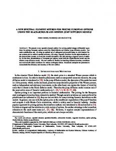
Because of Eq. (1), this choice gives a quadrature rule that exactly integrates the cardinal functions ψi . Since these functions are a basis for PN,M the cubature rule is exact for all g ∈ PN,M and thus for all g ∈ PN and so the cubature rule is at least of strength N . However, for some point sets, the Newton-Cotes quadrature formula will integrate a larger space and the cubature rule can be of strength 2N or higher. As mentioned in the introduction, for the 1-simplex and its tensor products, the LGL points of degree N are both optimal interpolation and cubature points. Thus a highly accurate method can be developed which results in a diagonal mass matrix since the interpolation and integration points are co-located; having a diagonal mass matrix is important for achieving efficiency. On the 2-simplex such points have not yet been found and thus far one must be content to choose either good interpolation or integration but not both. It should be noted that in previous works the Fekete points have been used as integration points which then results in a diagonal mass matrix [9], [13]; however, the cubature rule for Fekete points of degree N is only of strength N , and thus using these cubature points is a poor approximation to the degree 2N inner products which appear in the integral formulation of the equations. For some problems, cubature of strength N is insufficient to achieve exponential convergence. An example of what happens when Fekete points are used for both interpolation and integration is shown in Fig. 1 for test 3 given in Sec. 3. The dashed line denotes the solution obtained with Fekete points of degree N for interpolation and Gauss points for integration of strength 2N (to achieve a strength of 2N , the Gauss points are oversampled, meaning there are too many of them to be used to construct a degree N nodal basis). These two sets of points working in tandem give extremely good results where the error remains flat for long time-integrations; we shall refer to this approach as the FeketeGauss method. In contrast, the dotted line shows that when the Fekete points are used for both interpolation and integration, the fact that these points are only of strength N means that the error rises rather quickly and is significantly larger. The advantage of the latter strategy, however, is that the interpolation and integration points are co-located; that is, they are one and the same. This vastly simplifies the construction of the numerical algorithms because one need not interpolate onto another set of points in order to evaluate integrals. The fact that the interpolation and integration points are co-located means that the mass matrix will be diagonal and thereby will be trivial to invert; a non-diagonal mass matrix has been a thorn in the side of triangular spectral element methods and is the main reason why triangles have not been able to compete with quadrilaterals in terms of efficiency. From this discussion it seems logical to assume that to get around the current dilemma requires the construction of a new set of points for the triangle that have cubature strength of close to 2N while having reasonably low Lebesgue constants. In the next section we describe the approach used for constructing points that satisfy both of these two criteria. The solid line in Fig. 1 shows the results for these new cubature points; these points offer a similar accuracy to the Fekete-Gauss method while having the attractive property of the Fekete points, that is, a diagonal mass matrix. 4

−4

10

−5

Fekete−Gauss O(2N) Fekete O(N) Cubature O(2N)

2

φ Normalized L Error

10

−6

10

−7

10

−8

10

0

5

10

15 20 Time in Days

25

30

Fig. 1 Test 3: Shallow Water Equations. The normalized φ L2 error as a function of time in days for the Fekete-Gauss method with O(2N ) integration (dashed line), Fekete points with O(N ) integration (dotted line), and the cubature points with O(2N ) integration (solid line) integration for nI = 3 and N = 7 polynomials.

2.3 Computing Cubature Points Finding points with optimal cubature properties has been extensively studied independently of spectral element applications and has a long history of both theoretical and numerical development. For a recent review, see [14], [15], [16], and [17]. An on-line database containing many of the best known quadrature formulas is described in [18]. One successful approach for numerically finding quadrature formulas dates to [19]. A generalized version was used recently in [20]. Newton’s method is used to solve the nonlinear system of algebraic equations for the quadrature weights and locations of the points. Symmetry is used to reduce the complexity of the problem. The complexity can be further reduced with a cardinal function based algorithm [21]. If one consults the database and the newest numerical results in the above references, it appears that cubature points of degree N with strength 2N or even 2N − 1 do not exist in T . Furthermore, the best cubature formulas for T do not have sufficient points (if any) on the boundary of T . If a set of cubature points will also be used to construct the nodal basis in the space PN,M there must be N + 1 points along each edge of T . This is because the nodal basis must generate vertex, edge and interior modes, and the interior modes must be uniformly zero on ∂T (this is critical for the construction of C 0 approximations across element boundaries). If a cardinal function ψi ∈ PN,M is zero on N + 1 points on an edge of T then ψi (z) = 0 for any point z on that edge. This is because the restriction of any function in PN,M to that edge is a polynomial of degree N . Thus any ψi for zi in the interior of T is automatically an interior mode. Since the goal of achieving a cubature formula using points which interpolate PN and are of strength 2N − 1 is not achievable, we thus follow the ideas first put forth by Cohen et al. [11], [8] and Mulder [12]. Instead of working in PN , we use the enriched space PN,M with M > 0. A point set which can interpolate PN,M necessarily contains more points than those for PN . Thus there are more degrees of freedom which can be used to satisfy the system of cubature equations given in Eq. (2). The resulting points, which we call PN,M cubature points, are tabulated and compared against the two point sets used in the Fekete-Gauss method in Table I. The cubature points for N = 2 and N = 3 are due to Cohen et al. [11], [8] and degrees N = 4 and N = 5 are due to Mulder [12]. 5

To extend these results, we used the cardinal function cubature algorithm of [21]. Straightforward modifications were required, first to work with interpolation points for PN,M instead of PN , and second to impose that there be N + 1 points along each edge of T (for a total of 3N points along the perimeter). We were able to reproduce the previously computed results for degrees N ≤ 5 along with the two new degrees N = 6 and N = 7 which we list in Table III. In fact, higher degrees of N for either triangles or tetrahedra are achievable with this procedure.

N 1 2 3 4 5 6 7

K 3 6 10 15 21 28 36

Fekete-Gauss in PN K0 d 3 2 6 4 12 6 16 8 25 10 36 12 46 14

kIk 1.00 1.67 2.11 2.58 3.19 4.08 4.78

N 1 2 3 4 5 6 7

M 0 1 1 1 2 3 3

Cubature in PN,M K = K0 3 7 12 18 30 46 51

d 1 3 5 7 10 12 14

kIk 1.00 1.45 2.21 3.75 5.23 7.40 7.50

Table I Properties of the cubature points and the points used in the Fekete-Gauss method. N and M determine the polynomial space PN,M , K is the number of interpolation points, K 0 the number of integration points, d the strength of the integration points and k I k is the Lebesgue constant of the interpolation points.

Table I shows the number of interpolation points, K, integration points, K 0 , and the Lebesgue constant, k I k, for both the Fekete-Gauss and cubature points as a function of the polynomial degree, N . The first thing to notice about these two sets of points is that the Fekete-Gauss points have superior Lebesgue constants than the cubature points. However, this should not be surprising since the Fekete points are constructed in order to minimize interpolation error and the Lebesgue constant is a measure of the quality of the points to achieve good interpolation (a lower Lebesgue constant implies better interpolation). 2.4 Evaluating the Nodal Basis Functions To define the local operators which shall be used to construct the global approximation of the solution we begin by decomposing the domain Ω into Ne non-overlapping triangular elements Ωe such that Ne [ Ω= Ωe . e=1

We then further map the arbitrary triangles Ωe into the reference right triangle T . To perform differentiation and integration operations, we introduce the nonsingular mapping x = Ψ (ξ) which defines a transformation from the physical Cartesian coordinate system, x, within each triangle Ω e to a local reference coordinate system, ξ, in the reference right triangle T (see [7] for details on this mapping for curved elements in R3 ). Let us now represent the local element-wise solution q by its nodal expansion in PN,M as q(ξ) =

K X

q(ξ k )ψk (ξ)

k=1

where K = dim PN,M and the nodal basis functions ψk are defined as in Eq. (1). For the points (ξi , ηj ) we choose the newly derived cubature points which, while trivial to evaluate nodal basis functions, complicate any other operation such as the evaluation of their derivatives. Here we follow 6

[5] and represent the nodal basis functions in terms of the Proriol polynomials [22],[23] which in T are an orthogonal basis for PN,0 . Stable recurrence relations which can be used to evaluate these polynomials and their derivatives are given in [24]. Note that these polynomials are traditionally denoted with a double index (m, n) representing the top degree in ξ and η. But here we use a single index and denote them by ϕi , i = 1, . . . , dim PN . To generate an easily computable basis for PN,M we need to add additional basis functions for the interior modes in PN,M which are not in PN . For these polynomials we use the formulas given in [24],[2], and we denote them by ϕi , i = (dim PN + 1), . . . , K.

2.5 Filtering the High-Frequency Waves As with most high-order methods, when solving non-linear problems some filtering is needed to control the accumulation of aliasing errors. The ability to selectively filter only the highest wave numbers is an advantage of the spectral element method. However it does require that we use an expansion in only orthogonal Proriol polynomials, since a nodal expansion or an expansion that involves interior modes will not be orthogonal and thus not isolate the high frequency content to only the high wave number modes. Thus to implement filters, we need to compute the expansion of the local element-wise solution q in terms of only orthogonal Proriol polynomials. In order to prevent confusion with the augmented basis for PN,M , here we denote the basis for P(N +M ) by gi , i = 1, . . . , K1 , where K1 = dim P(N +M ) . Since q ∈ PN,M ⊂ P(N +M ) , q has a unique expansion in terms of g. Denoting this expansion by q(ξi , ηi ) =

K X

q˜k Ri,k

(3)

k=1

where q˜k are the Proriol coefficients of q and R is the rectangular Vandermonde matrix for the basis g, allows us to define the K × K1 rectangular Vandermonde matrix R by Ri,k = gk (ξi , ηi ). Note that the appropriate right inverse of R for filtering is constructed as follows: given the set of point values q(ξi , ηi ), the expansion in terms of ϕ (the basis for PN,M ) can be computed by applying V −1 , the inverse of the Vandermonde matrix. This polynomial is in P(N +M ) and thus has a unique expansion in terms of g (the basis for P(N +M ) ), and so we have a mapping from the set of point values q(ξi , ηi ) to the expansion coefficients q˜; let us denote this map by R r . Applying Eq. (3) to expansion coefficients computed with Rr must recover the original grid point values, and thus RRr = I where I is the identity matrix. In matrix form, we now write Eq. (3) as ˜ = Rr q. q

˜ q=Rq

(4)

We can now apply filters to q directly to its Proriol coefficients in P(N +M ) . There are many possible filters, but here, based on past experience [25], [7], we choose the Boyd-Vandeven transfer function [26] which we denote by Λ. Applying the filter to the amplitudes and then transforming to nodal (physical) space is achieved in the following matrix-vector multiply operation qF = F q where F = R Λ Rr 7

(5)

is the K × K filter matrix and is applied every time-step at full strength. However, in the original Boyd-Vandeven filter only the highest modes (polynomials of degree N + M ) are completely annihilated and this may be too severe for either quadrilateral spectral elements or exact integration triangular spectral elements. Thus the issue with the new cubature points is how to view the approximation space which these points span. For example, should one take the degree to be the degree of the edge modes N , or the degree of the interior modes, N + M ? Let us denote the order of the space which the filter acts on as NF . In Table II we show the values used for filtering the cubature points. As an example, for P7,3 the interpolation functions of the cubature points contain some degree 10 (N+M) modes. The filter then acts on all the degree 9 and 10 modes. Unfortunately, we currently have no theory to support our filter choices; the values listed in Table II were found experimentally but they appear to work for a variety of applications. Filtering for PN,M N 1 2 3 4 5 6 7

M 0 1 1 1 2 3 3

K 3 7 12 18 30 46 51

NF 2 3 4 5 6 8 8

Table II The indices N, M for the polynomial space, the number of cubature points K, and the highest mode unaffected by the filter, NF .

2.6 Integration and Local Element-wise Operators In order to complete the discussion of the local element-wise operations required to construct discrete spectral element operators we must lastly describe the integration procedure required by the weak formulation of all Galerkin methods. For any two functions f and g the integration I proceeds as follows Z K X I[f, g] = f (x) g(x)dx = wi | J(ξ i ) | f (ξi ) g(ξi ) (6) Ωe

i=1

where w are the cubature weights and J the Jacobians of the transformation from physical space to the local space of the reference element. Note that for straight-edged triangles J and all other metric terms are constant but not so for curved elements. To simplify the description of the numerical algorithm, let us define the following local element operators: let Z Mije =

Leij = Deij

Z

Ωe

=

Z

ψi (x)ψj (x)dx,

(7)

∇ψi (x) · ∇ψj (x)dx,

(8)

ψi (x)∇ψj (x)dx,

(9)

Ωe

Ωe

represent the mass, Laplacian, and differentiation matrices where i, j = 1, . . . , K. 8

Using Eq. (6) allows us to rewrite Eqs. (7), (8), and (9) as Mije = wi | J(ξ i ) | δij , Leij =

K X

(10)

wi | J(ξ i ) | ∇ψi (ξ i ) · ∇ψj (ξ i ),

i=1 Deij

= wi | J(ξ i ) | ∇ψj (ξ i ),

(11) (12)

where δij is the Kronecker delta function. As Eq. (10) shows, having the interpolation and integration points, ξ i , co-located results in the mass matrix, M e , being diagonal which significantly simplifies the construction of the global matrix problem and its solution. 2.7 Formulation of the Method We follow the generalized diagonal mass matrix spectral element formulation outlined in [9]. This method is based directly on the original DMM spectral element method proposed by [27] except that the domain is decomposed into triangular instead of quadrilateral elements and we are working in the space PN,M . The method proceeds as follows: by piecing together appropriate nodal basis functions in neighboring elements, a set of global functions can be constructed that are C 0 and piecewise polynomial. These global functions are used as the test functions in the weak form of the equations of interest, and the unknowns are expanded in terms of these global functions. The resultant integral equations are decomposed as a sum of integrals over each element. Finally, the quadrature rule associated with the points used to construct the cardinal function basis is used to evaluate each integral. Because of the nodal nature of the global functions, this results in much simplification, including giving a diagonal mass matrix. The result is a method which can satisfy the equations globally by simply summing the local element matrices, Eqs. (10), (11), and (12), to form their global representation [27]. This summation procedure is known as the global assembly or direct stiffness summation. Let us represent this direct stiffness summation (DSS) procedure by the summation operator Ne ^

e=1

with the mapping (i, e) −→ (I) where i = 1, . . . , K are the local element grid points, e = 1, . . . , Ne are the spectral elements covering the global domain, and I = 1, . . . , Np are the global grid points. Applying the DSS operator to the local element matrices results in the following global matrices: M=

Ne ^

M e, L =

Ne ^

Le ,

e=1

e=1

D=

Ne ^

De

e=1

where M , L, and D are matrices of dimension Np × Np and M is diagonal and thereby trivial to invert. 2.7.1 Poisson Equation on the Plane For the Poisson equation

∇2 q = f

we define its variational statement as: find q ∈

H01 (Ω)

−Lq = f 9

(13) 1

∀ ψ ∈ H such that (14)

where H01 (Ω) is the space of all functions (with zero Dirichlet boundary conditions) with functions and first derivatives belonging to L2 (Ω) - the space of all functions that are square integrable over Ω. The domain used for this test is x ∈ [0, 1] × [0, 1]. 2.7.2 Advection Equation on the Sphere Similarly, for the advection equation on the sphere ∂q + u · ∇q = 0 ∂t

(15)

we define the variational statement as: find q ∈ H 1 (Ω) ∀ ψ ∈ H 1 such that ∂q = −M −1 uT Dq. ∂t

(16)

On the sphere, however, no additional boundary conditions are required other than periodicity which is satisfied by the connectivity of the grid. 2.7.3 Shallow Water Equations on the Sphere The shallow water equations on the sphere are ∂q = S(q) ∂t

S(q) = −



∇ · (φu) u · ∇u + f (x × u) + ∇φ + µx

(17)



(18)

where q = (φ, uT )T , the nabla operator is defined as ∇ = (∂x , ∂y , ∂z )T , φ is the geopotential height (φ = gh where g is the gravitational constant and h is the vertical height of the fluid), u = (u, v, w) T is the Cartesian wind velocity vector, f = 2ωz a is the Coriolis parameter and (ω, a) represent the rotation of the earth and its radius, respectively. The term µx, where x = (x, y, z)T is the position vector of the grid points, is a fictitious force introduced to constrain the fluid particles to remain on the surface of the sphere (see [7] for details). Note that this equation set represents an initial value problem with no boundary conditions; the only condition required is that of periodicity which is imposed by the geometry of the spherical domain. The variational statement of the problem is: find (φ, uT )T ∈ H 1 (Ω) ∀ ψ ∈ H 1 such that ∂φ = −M −1 D T (φu) ∂t

(19)

∂u = −M −1 uT Du − f (x × u) − M −1 Dφ − µx ∂t

(20)

where for φ and u we choose the polynomial space PN,M -PN,M . 10

3 Numerical Experiments For the numerical experiments, we use the normalized L2 error norm sR − q)2 dΩ Ω (q R exact kqkL2 = q2 dΩ Ω exact

to judge the accuracy of the TSE methods. In addition, we compute the order of convergence as an average convergence rate computed over all the grid refinements where at each grid refinement, n I , the convergence rate is defined as rate =

log [errornI +1 /errornI ] . log [nI /(nI + 1)]

The grid refinement parameter nI determines the number of elements as follows: on the plane the number of elements are NE = 2n2I and on the sphere NE = 20n2I . Three equation sets are used to judge the performance of the DMM TSE method: elliptic (linear scalar) and hyperbolic equations (linear scalar and nonlinear vector). The elliptic (test 1) is solved on the plane while the hyperbolic equations (tests 2 and 3) are solved on the sphere. The reason why the topology of the domain is important is because a domain without curvature (such as the plane) can be tiled completely with straight-edged triangles while a domain with curvature must be tiled by curved triangles; the metric terms of straight-edged triangles are constant per element whereas for curved elements the metric terms vary with the position of the interpolation/integration points within the element. Thus the application of DMM TSE method on a curved manifold represents a very stringent test for judging the performance of this new method. In the next few sections we compare the results of the DMM TSE method using cubature points with those of the Fekete-Gauss method. The Fekete-Gauss method has been optimized to both interpolate and integrate with high accuracy. Therefore, these points represent the best possible solutions that one can achieve with nodal triangular spectral elements. While it is true that for curved elements the metric terms are no longer constant and therefore for exact integration one would require perhaps up to O(3N ) integration accuracy; however, because the difference between O(3N ) and O(2N ) integration is quite minimal we shall refer to the Fekete-Gauss O(2N ) as the best possible solution that one can achieve with nodal triangular spectral elements. Of special interest is whether or not the cubature points yield exponential (spectral) convergence; in other words, we are particularly interested if the following relation holds error ∝ O(∆xN +1 ) which states that the error decreases exponentially with grid refinement (∆x) for increasing polynomial order N . Thus for a method to possess spectral accuracy requires a convergence rate of order (N+1) for all values of N. 3.1 Test 1: Poisson Equation on the Plane The Poisson equation has the exact solution qexact = xa (1 − x)b y c (1 − y)d when the forcing function, f , is used to satisfy Eq. (13). The coefficients a, b, c, and d control the polynomial degree of the solution and for simplicity we take a = b = c = d = 3 which results in a 12th order polynomial which is more than sufficient to judge the accuracy of up to 7th order cubature points. Homogeneous Dirichlet boundary conditions are used and the Laplacian operator is inverted using the conjugate gradient method with point Jacobi iteration. 11

0

0

10

10

N=2

−4

10

Rate=3.44

10

−8

N=5 Rate=5.56

−10

10

−12

10

1

N=7 Rate=7.37

2

4 8 Grid Refinement (n )

−4

N=3

Rate= 4.03

−6

N=4 Rate= 4.81

−8

10

N=6 Rate=6.46

16

Rate= 3.16

10

N=4 Rate=4.50

10

Rate= 2.53 N=2

10

N=3 Rate=3.80

−6

N=1

−2

10

Rate=1.72

2

q Normalized L2 Error

N=1

q Normalized L Error

−2

10

−10

10 32

1

I

N=5 Rate= 5.43

N=7 Rate= 6.56

2

N=6 Rate= 5.94

4 8 Grid Refinement (n )

16

32

I

a)

b)

Fig. 2 Test 1: Poisson Equation. The normalized q L2 error for the a) Fekete-Gauss and b) cubature points TSE methods as a function of grid refinement, nI , for the polynomial degrees N = 1, ..., 7 with their associated convergence rates.

3.2 Test 2: Advection Equation on the Sphere The initial condition used for the advection equation is q(λ, θ, 0) = e−r

2

/ri2

where r = a cos−1 (sin θi sin λ + cos λi cos θ cos(λ − λi )) , ri =

a , 3

a is the radius of the sphere, and (λi , θi ) is the initial position of the wave in spherical coordinates; the exact solution can be found in [28]. The time-integration is handled by the explicit 2nd order backward difference formula proposed in [29]. While this test case also involves a linear scalar equation, as in test 1, the difference is that this equation is now hyperbolic with the additional degree of difficulty posed by the curved topology of the spherical domain; this curvature in the domain has major consequences because this means that the metric terms (e.g., Jacobians) are no longer constant.

3.3 Test 3: Shallow Water Equations on the Sphere To further test the accuracy of the DMM TSE method we use a system of nonlinear hyperbolic equations, that is, the shallow water equations on a rotating sphere. Similarly to test 2, this test also poses the additional difficulty of having to use curved elements in order to allow the elements to tile the surface of the sphere. The initial conditions used are those of case 2 in the Williamson et al. [28] shallow water test suite. Once again, the time-integration is handled by the explicit 2nd order backward difference formula. 12

0

0

10

10

−1

2

2

φ Normalized L Error

Rate=1.50

10

φ Normalized L Error

N=1

−1

10

Rate=0.91

N=1

−2

10

N=2 N=5 Rate=3.28

−3

10

−4

10

1

N=7 Rate=4.69

N=6 Rate=4.17

2

−2

10

Rate=1.83

N=7 Rate=4.84

N=3 Rate=2.85

4 8 Grid Refinement (n )

16

−4

10

32

I

N=3 Rate=2.18

−3

10

N=4 Rate=2.60

N=2 Rate=1.92

N=5 Rate=3.57

1

2

N=6 Rate=4.78

N=4 Rate=2.96

4 8 Grid Refinement (n )

16

32

I

a)

b)

Fig. 3 Test 2: Advection Equation. The normalized φ L2 error for the a) Fekete-Gauss and b) cubature points TSE methods as a function of grid refinement, nI , for the polynomial degrees N = 1, ..., 7 with their associated convergence rates.

3.4 Summary of Results Figures 2, 3, and 4 show the normalized L2 error as a function of grid resolution, nI , for various polynomial degrees for the Fekete-Gauss and cubature points for tests 1, 2, and 3, respectively. For test 1 (elliptic equation on the plane) the cubature points perform better than the FeketeGauss method for some degrees of N but do not do as well for others, especially for N ≥ 6. In fact, for this particular type of equation it makes little sense to use the cubature points over the Fekete-Gauss points because both methods require the inversion of a Laplacian and for this reason the cubature points have no advantage; note that the discrete weak-form Laplacian operator is in fact the well-known stiffness matrix. For test 2 (advection equation on the sphere) both methods failed to yield spectral convergence even though both methods converged at a rapid rate. However, both methods yield similar convergence rates which is a good result because it means that the cubature points behave similarly to the Fekete-Gauss points; recall that the Fekete-Gauss points represent the best that one can do with high-order nodal triangles. For test 3 (shallow water equations on the sphere) the results of the cubature points are quite similar to those of the Fekete-Gauss method (they both yield spectral convergence); this seems to indicate that the cubature points are a good replacement for the Fekete-Gauss points for systems of nonlinear hyperbolic equations. From these results one can see that overall the cubature points do quite well compared to the Fekete-Gauss points. The main reason for considering the cubature points is due to the fact that they yield a diagonal mass matrix which allows for the construction of efficient time-integration algorithms. To emphasize this point we show in Fig. 5 the L2 error (Fig. 5a) and wallclock time in seconds (Fig. 5b) as a function of polynomial order for test 3 for both the Fekete-Gauss and cubature point methods using grid refinement level nI = 3; these results were obtained on a Dell PC with an Intel Xeon 1.8 gigahertz processor. Figure 5a shows that both methods yield spectral convergence and that these errors are almost identical for both methods; however, Fig. 5b shows 13

0

10

0

−2

10

10

10

−6

N=5 Rate=6.06

10

N=7 Rate=7.31

10

1

2

N=6 Rate=6.89

Rate=1.96

−4

10

Rate=2.14

N=3 Rate=3.18

N=3 N=5 Rate=5.48

−6

10

N=4 Rate=4.05

4 8 Grid Refinement (n )

Rate=1.88

N=2

2

Rate=1.85

N=2

−4

φ Normalized L Error

2

φ Normalized L Error

N=1

−8

N=1

−2

10

N=7 Rate=7.36

16

−8

10

32

I

1

2

N=6 Rate=6.37

Rate=3.71

N=4 Rate=3.87

4 8 Grid Refinement (n )

16

32

I

a)

b)

Fig. 4 Test 3: Shallow Water Equations. The normalized φ L2 error for the a) Fekete-Gauss and b) cubature points TSE methods as a function of grid refinement, nI , for the polynomial degrees N = 1, ..., 7 with their associated convergence rates.

that the Fekete-Gauss points require far more computing time to achieve these results. The cost of the Fekete-Gauss method increases exponentially with either increasing grid resolution, n I , or polynomial degree, N . This is due to the Fekete-Gauss method having a sparse global mass matrix which must be inverted at every time step. Giraldo and Warburton [7] showed how to construct this type of nodal triangular spectral element and even with the use of static condensation and conjugate gradient iterative solvers the cost of the method could not be brought down. In contrast, the cubature points TSE method, having a diagonal mass matrix, allows for very simple and extremely efficient time-integration strategies precisely because it does not involve the inversion of a mass matrix. In this paper we have only discussed the repercussions that a diagonal mass matrix has on the efficiency of explicit time-integrators; however, these effects are most important in the construction of semiimplicit time-integrators which are used to increase the allowable time-step that a model can use while maintaining stability. Semi-implicit time-integrators play an important role in production-type models such as those used in numerical weather prediction (see [30]). Finally, in Fig. 6 we show the accuracy per computational cost for both the Fekete-Gauss (Fig. 6a) and cubature points (Fig. 6b) for test 3 for orders N = 1, ..., 7. For such a plot, the best results are those nearest the bottom left corner of the plots; that is, this means that the method yields high accuracy (low L2 error) with little computational cost. For the Fekete-Gauss points the polynomial orders N = 4 and N = 6 offer the best compromise between accuracy and efficiency. Although the results for these points are not very easy to interpret one thing is clear: orders N ≤ 3 are inferior to orders N ≥ 4. On the other hand, the results of the cubature points are much simpler to interpret. Note that orders N ≤ 2 are not very competitive with the high order points (N ≥ 3). The orders N = 3 and N = 4 give good results, but clearly orders N ≥ 5 are by far the best. From these three orders, as in the Fekete-Gauss points, order N = 6 offers the best compromise between accuracy and efficiency. In summary, the main point of this figure is that high order (in this case N = 6) is clearly far more efficient than the lower order methods. For example, to get an accuracy of 1 × 10 −6 the order N = 6 points will cost far less than the other polynomial orders. 14

400

0

10

Fekete−Gauss O(2N) Cubature O(2N)

Wallclock Time (seconds)

300

−2

10

250

2

φ Normalized L Error

Fekete−Gauss O(2N) Cubature O(2N)

350

−4

200

10

150

−6

100

10

50 −8

10

1

2

3 4 5 Polynomial Order (N)

6

0 1

7

2

3 4 5 Polynomial Order (N)

6

7

b)

a)

Fig. 5 The a) normalized φ L2 error and b) wallclock time as a function of polynomial order, N , for the Fekete-Gauss and cubature points TSE methods for a five day integration of test 3 using n I = 3 grid refinement.

−2

−2

10 φ Normalized L Error

−4

2

2

φ Normalized L Error

10

10

N=5 N=3

−6

10

N=2

−8

2

10 10 Wallclock Time (seconds)

N=2

N=5

−6

10

N=6 N=7

N=7 0

N=1

N=4

N=6

10 −2 10

−4

10

N=1

10 −2 10

4

10

a)

N=3

N=4

−8

0

2

10 10 Wallclock Time (seconds)

4

10

b)

Fig. 6 The normalized φ L2 error as a function of wallclock time for a) the Fekete-Gauss and b) cubature points for a five day integration of test 3 using N = 1, ..., 7.

4 Conclusions We have presented a promising new set of cubature points on the triangle which can be used both for interpolation and integration. The fact that the interpolation and integration are co-located means that the points yield a diagonal mass matrix (DMM). We presented implementation strategies of this DMM triangular spectral element (TSE) method for elliptic and hyperbolic equations on 15

planar and spherical surfaces. We compared the cubature points to the usual strategy of employing one set of points for interpolation (Fekete) and another set for integration (Gauss) which we call Fekete-Gauss TSE; this method, however, does not yield a diagonal mass matrix. The cubature points compared quite favorably with the Fekete-Gauss points especially for the system of nonlinear hyperbolic equations. In addition, these good solutions can be obtained quite cheaply with the cubature method because they yield a diagonal mass matrix which allows for simple and efficient time-integration strategies; this may now allow the triangular SE method to compete in terms of both accuracy and efficiency with the quadrilateral SE method while allowing far more flexibility in the choice of adaptive unstructured grids. Because the cubature points yield a DMM TSE, in future work we shall exploit this property to construct semi-implicit time-integrators for various hyperbolic equation sets on adaptive unstructured grids including: the Euler equations, and the primitive equations for both the atmosphere and ocean. Acknowledgements FXG was supported by the Office of Naval Research through program element PE0602435N. MAT was supported through the Sandia University Research Program. We would like to thank Tim Warburton for his assistance during the initial phase of this work.

References 1. A.T. Patera, A spectral element method for fluid dynamics - laminar flow in a channel expansion. Journal of Computational Physics 54 (1984) 468-488. 2. P. Solin, K. Segeth, and I. Dolezel, Higher-Order Finite Element Methods. Chapman and Hall/CRC Press (2003). 3. S.J. Sherwin and G.E. Karniadakis, A triangular spectral element method; applications to the incompressible Navier-Stokes equations. Computer Methods in Applied Mechanics and Engineering 123 (1995) 189-229. 4. J.S. Hesthaven, From electrostatics to almost optimal nodal sets for polynomial interpolation in a simplex. SIAM Journal on Numerical Analysis 35 (1998) 655-676. 5. M.A. Taylor, B.A. Wingate, and R.E. Vincent, An algorithm for computing Fekete points in the triangle. SIAM Journal on Numerical Analysis 38 (2000) 1707-1720. 6. T. Warburton, L.F. Pavarino, and J.S. Hesthaven, A pseudo-spectral scheme for the incompressible Navier-Stokes equations using unstructured nodal elements. Journal of Computational Physics 164 (2000) 1-21. 7. F.X. Giraldo, and T. Warburton, A nodal triangle-based spectral element method for the shallow water equations on the sphere. Journal of Computational Physics 207 (2005) 129-150. 8. G. Cohen, P. Joly, J.E. Roberts, and N. Tordjman, Higher order triangular finite elements with mass lumping for the wave equation. SIAM Journal of Numerical Analysis 38 (2001) 2047-2078. 9. M.A. Taylor, B.A. Wingate, A generalized diagonal mass matrix spectral element method for nonquadrilateral elements. Applied Numerical Mathematics 33 (2000) 259-265. 10. B. Helenbrook, Polynomial Bases Suitable for Mass Lumping on Triangles. International Conference on Spectral and High-Order Methods (ICOSAHOM) (2004). 11. G. Cohen, P. Joly, and N. Tordjman, Higher order triangular finite elements with mass lumping for the wave equation, in Proc. 3rd Int. Conf. on Mathematical and Numerical Aspects of Wave Propagation. Eds. G. Cohen, E. Becache, P. Joly, and J.E. Roberts (SIAM, Philadelphia, 1995). 12. W.A. Mulder, Higher-order mass-lumped finite elements for the wave equation. Journal of Computational Acoustics 9 (2000) 671-680. 13. D. Komatitsch, R. Martin, J. Tromp, M.A. Taylor, B.A. Wingate, Wave propagation in 2-D elastic media using a spectral element method with triangles and quadrangles. J. Comp. Acoustics 9 (2001) 703-718. 14. R. Cools and P. Rabinowitz, Monomial cubature rules since Stroud: a compilation. J. Comp. and Appl. Math. 48 (1993) 309-326. 15. J. Lyness and R. Cools, A survey of numerical cubature over triangles. Applied Mathematics 48 (1994) 127-150. 16. R. Cools, Constructing cubature formulae: the science behind the art. Acta Numerica 6 (1997) 1-54. 17. R. Cools, Monomial cubature rules since Stroud: a compilation - part 2. J. Comp. and Appl. Math. 112 (1999) 21-27. 18. R. Cools, An encyclopaedia of cubature formulas. Journal of Complexity 19 (2003) 445-453. Online database located at http://www.cs.kuleuven.ac.be/˜nines/research/ecf/ecf.html.

16

19. J. Lyness and D. Jespersen, Moderate degree symmetric quadrature rules for the triangle. J. Inst. Math. Appl. 15 (1975) 19-32. 20. S. Wandzura and H. Xiao, Symmetric quadrature rules on a triangle. Computers and Mathematics with Applications, 45 (2003) 1829-1840. 21. M.A. Taylor, B.A. Wingate, and L.P. Bos, A cardinal function algorithm for computing multivariate quadrature points. SIAM Journal on Numerical Analysis to appear (2006). 22. J. Proriol, Sur une famille de polynomes a ´ deux variables orthogonaux dans un triangle. C.R. Acad. Sci Paris 257 (1957) 2459. 23. M. Dubiner, Spectral methods on triangles and other domains. Journal of Scientific Computing 6 (1991) 345-390. 24. G.E. Karniadakis and S. J. Sherwin, Spectral/hp Element Methods for CFD, Oxford Univ Press (1999). 25. M. Taylor, J. Tribbia, M. Iskandarani, The spectral element method for the shallow water equations on the sphere. J. Comput. Phys. 130 (1997) 92-108. 26. J. Boyd, The erfc-log filter and the asymptotics of the Euler and Vandeven sequence accelerations. in A. V. Ilin and L. R. Scott (eds), Proceedings of the Third International Conference on Spectral and High Order Methods, Houston Journal of Mathematics, Houston, Texas, (1996) 267-276. 27. Y. Maday, A.T. Patera, Spectral element methods for the incompressible Navier Stokes equations. in: A. K. Noor, J. T. Oden (Eds.), State of the Art Surveys on Computational Mechanics, ASME, New York, (1987) 71-143. 28. D.L. Williamson, J.B. Drake, J.J. Hack, R. Jakob, and P.N. Swarztrauber, A standard test set for numerical approximations to the shallow water equations in spherical geometry. Journal of Computational Physics 102, (1992) 211-224. 29. G.E. Karniadakis, M. Israeli, and S.A. Orszag, High-order splitting methods for the incompressible Navier-Stokes equations. Journal of Computational Physics 97, (1991) 414-443. 30. F.X. Giraldo, Semi-implicit time-integrators for a scalable spectral element atmospheric model. Quarterly Journal of the Royal Meteorological Society 131 (2005) 2431-2454.

N 6

7

Number 1 3 3 3 3 3 6 6 6 6 6 3 3 3 3 3 6 6 6 6 6 6

x 0.3333333333333333 0.0000000000000000 0.4207074595153500 0.6975345054486999 0.5000000000000000 0.0484777152220000 0.1009333864342500 0.2688476619807000 0.3694234213017000 0.2841797219605000 0.1811513191269000 0.0000000000000000 0.1671653533624000 0.4799846082104500 0.2805588962964500 0.9336675298564999 0.0797278918581500 0.2013629039284500 0.3789551577387000 0.3428699782753000 0.2809834462433500 0.1321756636294500

y 0.3333333333333333 0.0000000000000000 0.1585850809708500 0.1512327472752000 0.0000000000000000 0.9030445695557999 0.0000000000000000 0.0000000000000000 0.0497413284926000 0.1685399500274000 0.0548913882427000 0.0000000000000000 0.6656692932752000 0.0400307835790500 0.4388822074071001 0.0331662350717500 0.0000000000000000 0.0000000000000000 0.0000000000000000 0.1406581918813000 0.0493368139566500 0.0499184036996000

weight 0.0340548001889250 0.0004842730760035 0.0177785008242257 0.0122972050038037 0.0032466690489985 0.0080400015624530 0.0020317308565252 0.0030227165121272 0.0171924926133297 0.0202547332903523 0.0142325352719635 0.0002270804834076 0.0215081779064107 0.0142371781018152 0.0236326025323162 0.0041445630524500 0.0011906918877981 0.0020909447779454 0.0026709648805728 0.0211675487584138 0.0139626184559205 0.0103757635344830

Table III The polynomial order, N , the number of cubature points, and the x and y value of the first two barycentric coordinates of the cubature points which correspond to this cubature weight. The third barycentric coordinate is defined such that the sum of all three coordinates is one.

17