Sep 13, 2010 - boundary curve with the Euler characteristic Ï of the region. ... vertices of all points of distance r and edges consisting of pairs (q, ... two-dimensional graphs G without boundary, like triangularizations of ... At each of a few chosen points, we have drawn the spheres of ... are two dimensional but not planar.
arXiv:1009.2292v1 [math.GN] 13 Sep 2010
A DISCRETE GAUSS-BONNET TYPE THEOREM OLIVER KNILL
Abstract. We discuss a curvature theorem for subgraphs of the flat triangular tessellations of the plane. These graphs play the analogue of ”domains” in two dimensional Euclidean space. P We show that the Pusieux curvature K(p) = 2|S1 (p)| − |S2 (p)| satisfies p∈δG K(p) = 12χ(G), where χ(G) is the Euler characteristic of the graph, δG is the boundary of G and where |Sr | the arc length of the sphere of radius r in G. This formula can be seen as a discrete Gauss-Bonnet formula or Hopf Umlaufsatz.
Dedicated to Ernst Specker to his 90th birthday. 1. Introduction For a domain D in theR plane with smooth boundary C, the Gauss-Bonnet formula or Umlaufsatz C K(s) ds = 2πχ(D) relates the curvature K(s) of the boundary curve with the Euler characteristic χ of the region. For a simply connected region G for which the boundary is a simple closed curve, the total boundary curvature is 2π. This Gauss-Bonnet type result is a form of Hopf ’s Umlaufsatz and relates a differential geometric quantity, the boundary curvature, with a topological invariant, the Euler characteristic. In differential geometry, curvature needs a differentiable structure, while Euler characteristic does not. It is the transcending property between different mathematical branches which makes Gauss-Bonnet type results interesting. We prove here a discrete version of a ”Hopf Umlaufsatz” [3] which is of combinatorial nature; curvature is an integer. The result applies to special two dimensional graphs which are part of a flat two dimensional background graph X, where the dimensionality is defined inductively. While the Euler characteristic is a topological notion, we need ”smoothness assumptions” to equate the total boundary curvature with the Euler characteristic. The curvature, we consider here is K(p) = 2|S1 | − |S2 |, where Sr (p) is the arc length of the sphere Sr (p) at the point p. The sphere Sr is a subgraph of G with vertices of all points of distance r and edges consisting of pairs (q, q ′ ) in Sr (p) such that q and q have distance 1. As we will explore elsewhere, for many compact two-dimensional graphs G without boundary, like triangularizations of polyhedra with 5 or 6 faces, the integral of the curvature K(p) = 2|S1 | − |S2 | over the entire graph is 60χ(D). The ”smoothness” assumptions are more subtle than correspondP ing results for K1 (p) = 6 − |S1 |. For the later, the result p∈G K1 (p) = χ(G) is Date: February 11, 2010. 1991 Mathematics Subject Classification. Primary: 05C10 , 57M15 . Key words and phrases. Graph theory, Gauss-Bonnet, Curvature. 1
2
OLIVER KNILL
essentially a reformulation of Euler’s formula and holds for any ”two dimensional graph” with or without boundary. We will look at a relation between the ”first order curvature” K1 and second order curvature K at the end of this article. P The main result in this paper is the formula p∈δG K(p) = 12χ(G) which holds for discrete domains G and for a second order curvature K. To do so, we need to specify precisely what a ”smooth domain” is. The background lattice X plays here the role of the two-dimensional plane. Its √ vertices can be realized as the set of points {k(1, 0) + l(1, 3)/2 | k, l integers }. The edges are formed by the set of pairs for which the Euclidean distance is 1. In the infinite graph X, every point p has 6 neighbors. Together with edges formed by neighboring vertices, these points form the unit sphere S1 (p), a subgraph of X. Similarly, any sphere S2 (p) of radius 2 in this discrete plane has length |S2 | = 12. The curvature K = 2|S1 | − |S2 | is zero at every point of the background lattice X.
0
0
-1 1 1
0
0
0
0
0
0
0
0
1 -1 1
0
0
1
1
1 -1 2 -2 2 -2 2 -2 2 -2 2 -2 2 -2 2 -1 1
1 -1 2 -2 2 -2 2 -2 2 -2 2 -2 2 -2 2 -1 1
1 -1 0 -1 1 1 -2 -2 1 -1 -1 1 0
1 0
2
0
1 1
1 1
0
0
0
Figure: Curvature computation. The numbers near each vertex indicate the curvature of the point. At each of a few chosen points, we have drawn the spheres of radius 1 and 2 in G. Adding up the curvatures over the boundary gives 12. If a point has as a neighborhood a disc of radius 2, the curvature is zero. 2. Topology of the planar triangular lattice A finite subset G of the triangular lattice X defines a graph (V, E), where V ⊂ X is the set of vertices in G and where E is a subset of edges (p, q) in X, pairs
A DISCRETE GAUSS-BONNET TYPE THEOREM
3
in X have distance 1 within X. We start by defining a dimension for graphs. To our best knowledge, this notion seems not yet have appeared, even so in the graph theory literature, several notions of dimension exist. The definition of dimension is inductive and rather general and does not require the graph to be a subset of X. Definition 1. A sphere Sr (p) in the subgraph G of X whose vertices consists the set of points in G which have geodesic distance r to p, normalized, so that adjacent points have distance 1 within G. The edges of the sphere graph Sr are all pairs (p, q) with p, q ∈ Sr (p) for which (p, q) is in G. A disc Br (p) in the graph G is the set of points q which have distance d(q, p) ≤ r in G. Definition 2. A vertex p of a graph G = (V, E) is called 0-dimensional, if p is not connected to any other vertex. A subset G of X is called 0-dimensional if every point of G is 0-dimensional in G. Zero-dimensionality for a graph means that it has no edges. A point p of G is called 1-dimensional if S1 (p) is 0-dimensional, where S1 (p) is the unit sphere of p within G. A finite subset G of X is called 1-dimensional if any of the points in G is 1-dimensional. A point p of G is called 2 dimensional, if S1 (p) is a one-dimensional graph. A subset G of X is called 2-dimensional, if every vertex p of G is a 2-dimensional point. The dimension does not need to be defined. For example, a point which has a sphere which contains of one and zero dimensional components has no dimension. One could define inductively a fractional dimension by adding 1 to the average fractional dimensions of the points on the unit sphere. As an illustration of the notion of dimension, lets look at the platonic solids as graphs. The cube and the dodecahedron are one dimensional. The isocahedron and octahedron are two dimensional. The tetrahedron is three dimensional, because the unit sphere of each point is 2 dimensional. The cube and dodecahedron become two dimensional after kising (stellating) their faces. The tetrahedron becomes 2 dimensional after truncating corners. Definition 3. A point p in G called an interior point of G if the sphere S1 (p) in the graph G is the same than the sphere S1 (p) in the background lattice X. In other words, for an interior point, the sphere S1 (p) is a one-dimensional graph without boundary. Definition 4. A point p of a two-dimensional graph G is a boundary point of G, if it is not an interior point in G but has a neighbor in G which is an interior point. For an interior point, the sphere S1 (p) is a closed circle, for a boundary point, the sphere S1 (p) is a union of one-dimensional arcs. Definition 5. The boundary of G is the set of boundary points of G. The interior of G is the set of interior points of G. Remarks: a) The set of subsets {A ⊂ int(G) } ∪ {G } defines a topology on G such that the interior of G is open and the boundary δG is closed. b) The interior of a two dimensional graph G is not necessarily a 2 dimensional graph. The disc of radius 1 in X for example is has a single interior point so that the interior is zero-dimensional.
4
OLIVER KNILL
c) Two dimensionality of a graph has no relation with ”being planar”. There are planar graphs like the tetrahedral graph which is three dimensional in our sense but which is planar. And there are graphs like triangularizations of a torus, which are two dimensional but not planar. d) Topologically, one can show that the triangular graph X is the only simplyconnected two-dimensional flat graph without boundary.
Definition 6. We call a subset G of X a domain if the following 5 conditions are satisfied: (i) G is a two-dimensional subgraph of X. (ii) Every point of G is either an interior point or a boundary point. (iii) The set of boundary points in G is a one-dimensional graph. (iv) If two vertices p, q in G have distance 1 in X, then (p, q) is an edge in G. (v) Two interior points in G with a common boundary points have distance 1 or are both adjacent to a third interior point.
The conditions (i),(ii), (iii) are natural. Condition (iv) assures that no unnatural ”fissures” can exist. Condition (v) assures that the connectivity topology of the domain and the connectivity topology of the interior set are the same.
Definition 7. A domain is called a finite domain, if it is a finite graph which is a domain. A domain is called a smooth domain, if it is a domain and its complement is a domain too.
Remarks: a) We could additionally require the interior of a domain to be two-dimensional but we do not need that. Actually, the proof of the main theorem becomes simpler if we do not make this assumption. It would just lift a difficulty on a different level. For us it will be important to look at the dimension of points in the interior of G. b) Some of these conditions for ”domains” have analogues in the continuum, where they are necessary for the classical Gauss-Bonnet to be true: we can not have ”hairs” sticking out of the domain for example. The closure of the complement of a domain is a domain too and we can not just leave out part of the boundary. Also in the continuum, it should not happen that parts of domains are tangent to each other. We also can not allow the boundary to be two-dimensional, like for the Mandelbrot set. c) For a smooth domain, we can look at the interior H ′ = int(G′ ) of the complement G′ of int(G). Then, the boundaries satisfy δ(G) = δ(G′ ). The three sets int(G′ ), int(G) and δ(G) = δ(G′ ) partition the graph X.
A DISCRETE GAUSS-BONNET TYPE THEOREM
5
0
12
1
-1 0
1
-1
2
2
0
1
1
0
-1 1 -1 0 1 -1 2 1 0 1 0 -2 1 0 0 -2 2 0 -1 2 -1 1 0 0 0 0
2 2
0
0
-1
0 1
2
0
0 0 0 0 0 0 0 0 1 -1 2 -1 1 -2 0 2 2 -2 -2 0 -2 0 1 -2 0 -2 1 0 -2 2 1 -2 1 2 -1 1 0 -1 0 0 0 0 1 -1
0
-1 1 0 0 0 0 0 0 0 0 0 1 0 0 0 1 0 1 0 0 1 1 0 2
0
0 -2 0
0 1
0
-1 1 0 0 0 0 1 -1 -1 1 0 0 0 -1 1 1 -1 0 0 1 -1 0 0 1 2 0
1 0 0
2 0
0 -2 0
0 -2 0 -2 -2 0 0 -2 -2 0 -2 0
0 0
-12
1
1
1
1
0
0
0 -2 0 -2 -2 0 0 -2 -2 0 -2 0
0
0
0 0
0
1
0
1
1
0 -2 0 -2 -2 0 0 -2 -2 0 -2 0
1 0 0 0 0 1
0 2 1 0 0 -1 1 0 0 -1 1 1 -1 0 0 0 1 -1 -1 1 0 0 0 0 1 -1
1 0 0 0 1 0 0 0 0 0 0 0 0 0 1 -1
Figure: Examples of domains. The number in the upper right corner is the total boundary curvature of the domain.
4
-12 0
0 0
0 0
0 -4 2
0
0
0
2 2
-4 0 0 0
1
-1
2
2
0
1
1
0
2
2
-4
1
-1 0
-4
0
-4
2
0
2 2
0
0
0
0
0
-3
0
-1 1
-4
-1
2
-1
0
0 -2
-1
0
0
0
0
0 0
Figure: Examples of graphs which are not domains. To the left, a set with 2, 1 and 0 dimensional points. It violates conditions (i). The second example is a set with both 2 and 1 dimensional points.
6
OLIVER KNILL
16
6
1
1
0
2
2 0 2
0
2
1
2
2
2
1
0
1
0 1
2
0
Figure: The left example is a two-dimensional set with no interior points and no boundary points. It violates condition (ii). The second one violates (v).
16
2
0
2
0 4
0
22
0
4
1
2
0
2
2
2
4 4
2
2 2
2
1
0
Figure: Examples of graphs which are not domains. The first violates (v), the third violates (iii).
A DISCRETE GAUSS-BONNET TYPE THEOREM
7
16
10 2
1 2
-1 2
1
1
2 0
2
0 2
1
0
0
2 1
-1
0
1
2
1
2 2
1 0
-12 0
1
1
0
1
1
1
-4
0 1
1
-4
-4
0
-4 -4
1
-4
1
1 0
1
1
0
Figure: Domains which are not smooth domains. The curvature of the first was computed while assuming the nearest neighbor connection to be an edge as required by condition (iv). If the connection is not in place (violating (iv)), the total curvature would be 24. The following lemma allows us to deal more efficiently with eligible regions and eliminates many subsets which are not regions. It says that the set of interior points determines the region as well as its boundary. Lemma 1.SLet G be a domain and H = int(G) be the set of interior points of G. Then G = q∈H B1 (q), where B1 (q) is the disc of radius 1 in X. Especially, the interior set H = int(G) determines the domain G completely. Proof. If a point p is in G, then it is either S an interior point or a point adjacent to an interior point. Therefore G ⊂ q∈H B1 (q). On the other hand, if p is S in q∈H B1 (q), then p ∈ B1 (q) for some q. Because q ∈ G and S1 (q) ∈ G by definition of being an interior point, we have p ∈ G. � Remark: For a simply connected region, also the boundary of G determines the region, but we do not need that.
8
OLIVER KNILL
3. Curvature Definition 8. Let |Sr (p)| denotes the number of edges in the sphere Sr (p). We call it the arc length of the sphere Sr . Remarks. a) Note that |S1 | is not necessarily the number of vertices in S1 . Similarly, |S2 | is the number of edges in S2 which is not always equal to the number of vertices in S2 . b) The sphere |S1 | does not necessarily have to be connected, nor does it have to have a defined dimension. It could be a union of a segment and a point for example. Definition 9. The curvature of a boundary vertex p in a region G is defined as K(p) = 2|S1 (p)| − |S2 (p)| . The curvature of a finite domain G is the sum of the curvatures over the boundary. Remarks. a) This definition is motivated by differential geometry since one can derive an |−|S2r | analogue formulas in the continuum K = limr→0 2|Sr2πr for a point on the 3 boundary curvature of a region. b) Note that as defined, S2 (p) refers to the geodesic circle of radius 2 in G and not in X so that every point q ∈ G of distance 2 in X to p belongs to S2 (p) whether there is a connection within G from p to q or not. The reason for this choice is that we do want the curvature definition to be nonlocal. This subtlety will not matter since for the definition of smooth curve, we anyhow disallow situations where points have a large distance within G but small distance in X.
20
24
2
2
2
2
2
2 2
2
2
2
2
2
2
2 2
2
1 1
1
2
1
2 2
2
Figure: The first picture is a smooth domain. It is not simply connected although the two parts S1 , S2 of the regions are at first separated enough to get a curvature 24. In the second case S2 ”feels” part of the other region S1 and the curvature is not a multiple of 12.
A DISCRETE GAUSS-BONNET TYPE THEOREM
9
22
2
12
1
2
2
2
0
4
1
1
4
0
2
1
1
2
1
1
1
2
1
1
2
Figure: In the first picture, the domain is still not smooth because the complement is not a domain. The last example is a smooth domain. It has become simply connected. Definition 10. A curve γ in a smooth domain G is a sequence of points x0 , . . . , xn in the interior of G such that d(xi , xi+1 ) = 1 and consequently (xi , xi+1 ) is an edge of G. A curve is a closed curve if x0 = xn . In graph theory, a curve is called a chain. It is a nontrivial closed curve if its length is larger than 1. It is called a simple closed curve, if all points x0 , x1 , . . . , xn−1 are different and x0 = xn . Definition 11. A domain is called simply connected if every closed curve {x1 , . . . , xn } in the interior H of G can be deformed to trivial closed curve within G, where a deformation of a curve within G consists of a composition of P finitely many elementary deformation steps {x1 , . . . , xn } → {y1 , . . . , yn } with i d(xi , yi ) = 1 and such that xi , yi are in H. As in the continuum, simply connectedness means that any closed curve in the interior of G can be deformed to a point within the interior of G. 4. The curvature 12 theorem Our main result of this paper is a discrete version of the ”Umlaufsatz”. It will be generalized to more general domains below. Theorem 2 (Curvature 12 Umlaufsatz). The total boundary curvature of a finite, smooth and simply connected domain G is 12. Proof. For the proof, it suffices to look at local deformations. We start with an arbitrary simply connected smooth region G and find a procedure to remove interior points near the boundary while keeping the simply connectedness property and keeping also the curvature the same. Removing one point only affects the curvatures in a disc of radius 2 so that only finitely many cases need to be studied: Lemma 3 (Curvature is local). Let G1 , G2 be two regions and p be a point in both G1 and G2 . Let U1 = B2 (p) ⊂ G1 and U2 = B2 (p) ⊂ G2 be the discs of radius 2 in G1 and G2 respectively. Define Hi = Gi \ {p}. If U1 = U2 , then X X X X K(p) − K(p) = K(p) − K(p) . p∈H1
p∈H2
p∈G1
p∈G2
10
OLIVER KNILL
In other words, if we remove a point from a region, then the total curvaturechange can be read off from the curvature-changes in a disc of radius 2. We could check all possible configurations in discs of radius 2 and compare the total curvature before and after the center point is removed. We indeed checked with the help of a computer that in all cases, where the total boundary curvature changes, the number of local connectivity components of the interior has changed or the complement has become non-smooth near the removed point. These experiments helped us also to get the conditions what a domain is. But checking all possible local deformations is not a proof. We also need to know that there is always a point which we can remove without changing the topology of G or its complement. It turns out that this question is of more global nature. Take a ring shaped region for example which has a one dimensional interior. No point can be removed without the curvature to change. The key is to look at the dimension of points in the interior of G and distinguish points which are one-dimensional in int(G) and points which are two-dimensional in int(G). A zero dimensional interior means for a simply connected region that the graph is the disc of radius 1 in X. By removing interior points, we want to reach this situation.
12 0 1 0 1 0 1 1 0 0 1 2 1 1 1 1 0 0 0 1 1 1 0 0 -1 0 0 0 0 1 0 0 -1 0 -1 1 0 0 0 0 -1 0 0 0 0 0 0 0 0 -1 0 -1 0 0 1 -1 0 -1 0 1 -1 0 -1 0 1 0 1 1 0 1 0 1 0 -2 -1 -2 -1 1 0 -1 0 0 0 -1 0 0 -1 0 0 0 -1 0 0 1 0 -1 0 0 0 -1 0 0 -1 0 0 0 -1 0 0 -1 -2 -1 -2 1 1 0 1 0 0 1 0 1 0 -1 0 -1 1 0 -1 0 -1 1 0 -1 0 -1 0 0 0 0 0 0 0 0 -1 0 -1 0 0 1 -1 0 -1 0 1 -1 0 -1 1 0 1 0 0 -1 0 -1 1 1 1 1 0 0 0 0 1 1 1 1 0 0 0 0 1 1 1 1 0 1 0 1 0 0 1 0 1 0
0 1 0 1 0 1 0 1 0
Figure: Pruning a tree, a simply connected domain. To reduce a region, we have to trim the tree, removing alternatively two-dimensional interior points and onedimensional interior points until only one interior point is left.
A DISCRETE GAUSS-BONNET TYPE THEOREM
11
We are allowed to look at the topology of interior points because int(G) defines G by the above lemma, it is enough to check what happens if we remove interior points. Our goal is to show:
Proposition 4 (Trimming a tree). For any simply connected smooth region G for which the interior set H has more than one point, it is possible to remove an interior point p from H, such that the new region defined by H \ {p} remains a simply connected smooth region with one interior point less and such that the curvature does not change. The theorem follows from this proposition. Lets introduce some terminology: Definition 12. Given a smooth, simply connected region G with interior H. Denote by H1 the points in H which are one dimensional in H. Similarly, call H2 the set of points in H which are two dimensional in H. Connected components of H1 are called either branches or bridges. Connected components of H2 are called ridges. A branch of G is a connected component of H1 for which at least one point has only one interior neighbor. All other connected components of H1 are called bridges.
12 0 1 0 1 0 1 1 0 0 1 1 0 0 1 1 -1 0 0 1 -1 0 -1 1 0 0 -1 0 0 0 0 -1 0 0 1 0 1 0 0 1 -1 0 -1 0 1 0 1 0 1 1 1 0 1 1 0 -1 -1 -2 -1 0 1 0 -1 0 0 0 -1 0 0 -1 0 0 0 -1 0 1 0 0 1 0 -1 0 0 0 -1 0 0 -1 0 0 0 -1 0 1 0 -1 -2 -1 -2 0 1 1 0 1 0 1 0 1 0 1 0 -1 0 -1 1 0 -1 0 -1 1 0 0 -1 0 -1 0 0 0 0 0 0 0 0 -1 0 -1 0 0 1 -1 0 -1 0 1 -1 0 -1 1 0 1 0 0 -1 0 -1 1 1 1 1 0 0 0 0 1 1 1 1 0 0 0 0 1 1 1 1 0 1 0 1 0 0 1 0 1 0
Figure: A simply connected region with ridges, bridges. All branches have been pruned. Now, we have to start etching the ridges. We have the choice of 4 end ridges here. The simply connectivity assures that there is an end ridge.
12
OLIVER KNILL
12
2
2
2
2
2
2
Figure: The only situation, where we can not trim any more one dimensional branches nor two-dimension ridges. The set int(G) is the union of points which are two-dimensional in int(G) and points which are one-dimensional in int(G). We will use two procedures called pruning and etching to make the region smaller. The pruning procedure removes a one-dimensional interior point at branches. The etching procedure removes a two-dimensional interior point at ridges.
12 10 10 10 112 121 02-2 -1 1 -2 0 10 1 0-10 -2 0 -1 -1 11 121
12 0 10 21 102 12 11 2-2 1-2-1 0 -2 0 0 1 0-1-1 0 -1 11 121
12 121 02-2 10 210 10 1 10-2 -1-1 0 -1 11 121
12 0 12 11 2-2 1-11 01 0 1 0-1-1 0 01 11 21
12 121 02-2 11 10 1 10-1 0 1 12
12
12
12 121 02-2 10 10 1 10-1 -110 221
12 121 02-2 10 1 21 012
12 0 12 20 22 012
12 12 121 02-2 00 001 10 1 10-2 -1-1 0 -1 11 121
121 02-2 10 10 1 10-1 -100 111 12
0 12 11 2-2 101 0 1 0 1 12
12 121 02 01 11 12
12 11 211 121 02-2 -1 1 -2 0 10 1 0-10 -1 0 -1 -1 11 121
12 121 02-1 10 2 211
12 122 121 12
12 222 222
A DISCRETE GAUSS-BONNET TYPE THEOREM
13
Figure: Pruning reduces the lengths of branches. Since curvature is local, we only need to check for a few end situations that the total curvature does not change. Lets start with the pruning procedure which removing interior points which are one-dimensional in int(G). It allows us to remove one-dimensional branches until we can no more reduce one-dimensional points in int(G). Removing onedimensional parts will make sure that there will be a two-dimensional ridges ready for the etching procedure. Here are the situations which can occur locally at a point of a branch.
12
1
2
1
2
2
1
2
1
Figure: A one-dimensional point which has 1 interior neighbor. After removing a boundary point, we end up with region 0.
12
12 2
1
1
1
1
2
1
2
1
1
1
1
0
2
0
2
2
0
2
1
Figure: Reducing a one dimensional point at the boundary. For any of the two situations, we end up with a region with one interior neighbor.
14
OLIVER KNILL
12
12 1
1
1
0
1
1
2
1
0
1
2
-1
2
2
1
2
2
0
1
12
0
2
2
-1
2
0
0
2
0
2
0
2
1
2
0
2
0
Figure: For any of the first 3 situations, we end up with two neighboring interior points. After reducing one dimensional branches, the tree still can have one dimensional parts: these are 2D ridges connected with one-dimensional bridges which can not be pruned without changing the topology.
12 0 1 0 0 1 11 01 1 1 11 1 0 0 1 010
12 0 1 0 1 02 01 0 1 11 1 0 0 1 011
12 0 1 0 1 11 01 1 1 11 1 0 1 010
12
12
12 0111 01 101 1 11 1 0 1 10
12 0 2 10 01 -1 2 1 11 1 1 02
12 11 01 210 11 1 2 01
0 1 0 1 11 01 0 1 11 1 0 0 1 110
0 1 1 10 01 -1 2 1 11 1 0 1 02
020 01 210 1 11 1 1 01
12
12
12
12 021 01 11 111 2 010
0 1 0 1 10 01 2 1 11 1 0 0 1 0-1 2
0 1 1 02 01 0 1 11 1 0 1 011
0111 01 011 1 11 1 1 01
12
12 021 01 101 1 11 1 1 10
12 12 01 20 111 2 0-1 2
12 12 01 01 111 2 110
Figure: Etching thins out ridges. The etching is done at ridges which are end ridges, where only one bridge is attached. With too many bridges attached, the etching process might not work. The etching procedure is invoked if no one-dimensional branches are left. The region consists now of two-dimensional ridges connected with bridges. Our goal is to see that we can remove a two-dimensional interior point of a ridge.
A DISCRETE GAUSS-BONNET TYPE THEOREM
15
The simply connectivity implies that there is a ridge which has only one bridge connected to it. To see this, look at a new graph, which contains the two-dimensional ridges as vertices and one-dimensional bridges as edges. This graph has no closed loops and is connected and must be a tree with at least one end points. We can consequently focus our discussion to such an end-ridge for which only one 1dimensional bridge is attached. We are able to remove a boundary point on the opposite side of that region, where no branches can be and where the boundary is ”smooth”.
12 1
1
2
2
1
1
1
2
1
Figure: Reducing a two-dimensional interior point at the boundary which has 2 interior points as neighbors.
12 1
2
0
1
2
2
1
0
2
1
Figure: Reducing a two-dimensional point at the boundary which has 3 interior points as neighbors.
16
OLIVER KNILL
12 1
1
1
2
1
1
1
2
2
0
0
Figure: A situation where the point has 3 interior neighbors and where the point can not be reduced.
12 0
0
1
2
2
1
1
2
2
1
0
0
Figure: A situation, where the point has 4 interior neighbors and where the point can not be removed.
A DISCRETE GAUSS-BONNET TYPE THEOREM
17
12 1
1
1
2
1
0
1
2
1
2
0
Figure: A situation, where the point has 4 neighbors which are interior points and where the point can not be removed.
12 0
0
1
2
2
2
0
0
2
2
0
1
Figure: Four interior points bounding an interior point. The middle point can not be removed while keeping the region a smooth region.
18
OLIVER KNILL
12 0
2
0
2
2
0
0
2
2
0
2
0
Figure: Having exactly 5 interior points bounding an interior point is not possible. We then necessarily have 6 neighbors.
12
12 2
1
1
1 1
1 0 0
1
1
0
1
0 1
0
1
1
0
1 -1
1
0
0 -1 0
0 -1 0 1
0 0
1
0
1
0
0
0 -1 0
1 0 1
0
1
-2
1
1
0 -1 0
0 -1 0
1
1
1
1
0 -1 0
0 -1 0
1
1
2
2
1 0
0
-2 1 0
1
-1
0 0
-1 0 -1 0
1 0
-1 0 -2 0
-1
0
1
0 -1
1
2
1 0
-2
0
-2 0
0 0 -2 0
-1 0
-1
1
0
1
1 2
1
-1 0
-1 0
1 1
1 1
2
Figure: A bridge and branches. For the picture with the bridge, no interior point which is one-dimensional in int(G) can be removed. For the picture with the branches, no interior point which is two-dimensional in int(G) can be removed. This is a situation, where the branches first need to be trimmed. Once the etching process is over, we can again start pruning branches, or we are left with a region with only one interior point. If a region G can no more be pruned and edged then H consists of only one point and G consists of only 7 points and in this case, we know the total curvature is 12. Since pruning and etching did not change the curvature and we have demonstrated that one can reduce down every simply connected region to a situation with one interior point, this completes the proof of the curvature 12 theorem. �
A DISCRETE GAUSS-BONNET TYPE THEOREM
19
5. Discrete Gauss-Bonnet To generalize the Umlaufsatz to domains which are not necessarily simply connected we first define the Euler characteristic of a region using Euler’s formula: Definition 13. A face in a domain G is a triangle (p, q, r) of 3 points in G for which all three points have mutual distance 1. An edge in G is a pair p, q of points in G of distance 1. A vertex is a point in G. Denote by f the number of faces in G, by e the number of edges and v = |G| the number of vertices. The Euler characteristic χ(G) of the domain G is defined as χ(G) = v − e + f . Example: for a simply connected region, the Euler characteristic is 1. Lemma 5. The Euler characteristic does not change under the pruning and etching operations defined above: both removing an end point of a one dimensional branch, as well as removing a two dimensional point from a ridge does not change it. Proof. The number of interior points of a smooth region is 2f − e + χ and which can be proved by adding faces: each face added is equivalent to adding 2 edges. �
0 0
1
0
1
0
-2
0
0
1
1
0 1
-2
0
0
0 1
0 -2
0
1
-2
0 1
-2 0
-2
0
0
1
1 0
1
0
1
0
Figure: A region, where no interior point can be removed any more and which has more than one interior point is not simply connected. Remark. The Euler characteristic of int(G) and G is the same if G is a smooth region. Theorem 6 (Discrete Gauss-Bonnet theorem). If G is a finite smooth domain G with boundary C, then X K(p) = 12χ(G) . p∈C
We could use the same pruning-etching technique as before. However, pruning and etching can lead to final situations which have no end points like a ring. Instead of classifying all these final situations, it is easier to reduce the general situation to a simply connected situation. There are two ways, how to change the topology: • build bridges between different connected components.
20
OLIVER KNILL
• fill holes to make the region simply connected Merging different unconnected components is no problem. As long as their complement is a smooth region too, both the Euler characteristic as well as the total curvature add up. 1. We can assume the region to be connected, because both curvature as well as Euler characteristic are additive with respect to adding disjoint domains. To illustrate this more, we can also join two separated regions along with a one dimensional bridge. The curvature drops by 12, the number of connected components drops by 1.
24
0 1 1 0 1
0 1 1 0 0
1
0 0 -1 0 1 1
0 1 1
0 0 1 1 0
12
0 -1 0 1 1
2
2
0 1 1 0 1
1
1 1 0 -1 0
1
1 1 0 -1 0
1
0 0
1 0 1 1 0
0 1 1 0 0
0
1
0 -1 0 0 0 0 0 0 0 0 0 0 -1 0
1
0 -1 0 0 0 0 0 0 0 0 0 0 -1 0
0 1
0 0 1 1 0
1 1 0 1
0
1 0 1 1 0
Figure: Joining two regions changes the total curvature by 12.
Definition 14. The interior of a hole W is a bounded simply connected smooth region such that int(W ) is a component of the complement of G. By definition a whole W and the region G share a common part of the boundary.
By the Umlaufsatz for simply connected regions, the hole has total curvature 12. A key observation is that the point-wise curvatures at the inner boundary of G enclosing the hole are just the negative of the corresponding point-wise curvatures of the hole. This follows almost from the definition of curvature and the fact that the circles |S1 (p) ∩ W | + |S1 (p) ∩ G| = 6 and |S2 (p) ∩ W | + |S2 (p) ∩ G| = 12 so that KW (p) + KG (p) = 0.
A DISCRETE GAUSS-BONNET TYPE THEOREM
21
12 0
1
0
0
0
1
12
0
1
1
0
0
0
0
0
0
2
-1
1
2
-1
0
1
1
0
1
2
0 1
0
1 0
0 0
0 2
2
0 0
0
0 1
1
0
1
0
1 0
1
0
0
0
1
0
0 0
1
0
0
0
1
0
1
1
0
0
0
0
0
1
-2
-1
1 0
0 -2
1
0
-1
-2
-2
-2
0 1 0
1 0
0
-1
0
-1
0 1
0
0
0
0 0
0 1
1 0
1
0
0
0
1
0
Figure: Filling a simply connected hole from a larger region adds to the curvature exactly the same amount than the total curvature of the hole. The reason is that the point-wise curvatures of the removed inside region matches exactly the curvatures of the inner outside region if the inside region and the outside region have a common one-dimensional boundary. This shows that if we fill a hole, the total curvature increases by 12. Simultaneously, the Euler characteristic increases by 1. Alternatively, we could also cut rings:
22
OLIVER KNILL
4 0
1
0
1
0
1
0 1
0
0
1 0
10
-2
0
1
-2
-2
-2
-2
0 1 0
0
-2
0
1
0
1
1
4
0
1
0
-2
0
0
-1
-2
0
-2
-2
4 3
0
1 0
1
0 1
-1
1
0
2
0 -1
2
1
1
0
-2
0
1
0
1
0 1
1
0
2
1 0
0
8 0
1
0
1
0
1
0 2
0
0
1 0
12
-2
1
1
-2
-1
1
-2
-1
1
0
-2
1 2
0
1
0
1
0
-2
1
0
1 0
2
0 1
1
1
1
-2
0
0
0
2
0 1
0 1
1
1
-2 0
0
-1
1
1
1
0
1
1
1
0
2 0
Figure: When cutting a ring, the curvature changes from 0 to 12. Only the last region is a smooth region. The second last is a region but not smooth because the complement is not a region.
6. Compact flat graphs If we introduce identifications in the hexagonal background graph X, the topology of the background space changes. Identifying points along two parallel lines for example produces a flat cylinder. With a triangular tiling, we can tessellate a torus. Because there is no boundary now, the sum of the curvatures is zero, which is the Euler characteristic. Note that there are many different non-isometric graphs which lead to such tori. We call them twisted tori. As graphs they are different even if the number of faces, edges and vertices are fixed.
A DISCRETE GAUSS-BONNET TYPE THEOREM
23
Figure: A flat torus obtained by identifying opposite sides of a rectangular domain in a hex lattice. The total curvature is zero. The notion of regular domain can be carried over to discrete manifolds like the twisted tori just mentioned. Let X be such a twisted background torus. We assume that it is large enough so that S2 (p) is a circle at every point. Let G be a subgraph of X defined as before. We still have: Theorem 7. If G is a domain in a background torus X, then X K(p) = 12χ(G) . p∈δG
Remark: More flat compact graphs can be obtained using ”worm hole” constructions. Let X be a possibly twisted torus as defined above and let p,q be two points for which the discs Br (p) and Br (q) are disjoint and the spheres Sr (p) and Sr (q) are circles. Any orientable graph isomorphism between Sr (p) and Sr (q) produces an identification of points in G = X \ Br−1 (p) ∪ Sr (p) \ Br−1 (q) ∪ Sr (q). Without identification, the total curvature of the boundary of the domain G is P p∈C K(p) = 12χ(G) = −24 because every removed disc produces curvature −12. 7. Combinatorial curvature In this section, we consider a more elementary Gauss-Bonnet formula. The curvature is again defined by a Puisaux discretization, but only circles of length 1 appear in the definition. It is a first order curvature. Definition 15. For a two dimensional graph with boundary, we define the combinatorial Puiseux curvature as for interior points and for boundary points.
K1 (g) = 6 − |S1 (g)| K1 (g) = 3 − |S1 (g)|
For this combinatorial curvature, Gauss-Bonnet is much easier. For subgraphs of hexagonal lattice the boundary curvature is almost trivially equal to 6 because the curvature is related to angles of the corresponding polygon: for a boundary
24
OLIVER KNILL
P point, K1 (p)π/3 is the interior angle of the polygon. Because p K1 (p)π/3 = 2π P by the polygonal version of the Umlaufsatz, we have p K1 (p) = 6. Actually, Gauss-Bonnet holds in great generally for arbitrary two-dimensional graphs with or without boundary. Since it is so closely related to the Euler characteristic, we should the attribute it to Euler, even so we are not aware that Euler considered K1 (g), nor that he looked at the dimension of a graph.
Theorem 8 (Combinatorial Gauss-Bonnet). Assume G is a two-dimensional finite graph for which the boundary is either empty or forms itself a one dimensional set. Then X
K1 (g) = 6χ(G) .
g∈G
Remarks. 1) This result does not need the rigid requirements on the ”domain” as before nor does the graph have to be part of X; it works for any two-dimensional graph, with or without boundary. 2) The result appears in a different formulation, which does not make its GaussBonnet nature evident:Pthe Princeton Companion to Mathematics [2] mentions on page 832 the formula n (6 − n)fn = 12, where fn is the number n-hedral faces and summation is over all faces. This is an equivalent formulation, but it makes the Gauss-Bonnet character less evident. Note that the combinatorial Gauss-Bonnet theorem is entirely graph theoretical. It avoids the pitfalls with the definition, what a polyhedron is [4]. (Common definitions of ”polyhedra” refer to an ambient Euclidean space or impose additional structure on a graph). We can take a general finite graph which is two-dimensional at each point. Its points are either boundary points, points where the unit sphere is one-dimensional but not closed, or an interior points, where the unit sphere is a circle, a simple closed graph without boundary.
Proof. Assume first that the graph G has no boundary. For a two-dimensional graph, all faces necessarily are triangles. Therefore, the number of faces f and the number of edges e are related by the dimensionality formula 3f = 2e . Furthermore, we have the edge formula X g
|S1 (g)| = 2e
which is obtained by counting edges in a different way.
A DISCRETE GAUSS-BONNET TYPE THEOREM
25
P Figure: the identity g |S1 (g)| = 2d. Figure: the identity 3f = 2e. Using the definition of the Euler characteristic, and these two formulas, we compute 6χ(G) = =
6f − 6e + 6v = −2e + 6v X X X − |S1 (g)| + 6v = − (|S1 (g)| − 6) = K1 (g) . g∈G
g∈G
g∈G
This finishes the proof in the case of a graph without boundary. The case with boundary can be reduced to the boundary-less case: The boundary is a union of closed cycles. For each of these m cycles δGi just add an other point Pi and add n = |δGi | edge connections from each of the cycle boundary points of Gi to Pi . This produces a graph H without boundary and which contains G as a subgraph. The formula without boundary shows that 6χ(H) is the sum of curvatures of the original interior points and the sum of the curvatures of the boundary points as well as the sum of the curvatures K1 (Pi ) = 6 − ni to each newly added point Pi : X X X (6 − ni ) . K(g) + KH (g) + 6χ(H) = g∈δG
g∈int(G)
i
We also have χ(H) = χ(G) + m − |δG| + |δG| = χ(G) + m .
For boundary points, KH (g) = 6 − |S1 (g)| − 2 and KG (g) = 3 − |S1 (g)| so that KH (g) − KG (g) = 1. From the previous boundary less case, we get 6χ(H) =
X
g∈H
KH (g) =
X
KG (g)+
m X X
i=1 g∈δGi
g∈int(G)
so that χ(G) = 6χ(H) − 6m =
(KG (g)+1)+(6−ni ) =
X g∈G
K(g) + 6m − 6m =
X
K(g)+6m
g∈G
X
K(g) .
g∈G
� The just verified combinatorial Gauss-Bonnet is entirely graph theoretical. Our curvature definition K was motivated from the notion of Jacobi fields in the classical case given by second derivatives. While ”smoothness” requirements” are necessary for the more sophisticated Gauss-Bonnet formula, the just mentioned metric Gauss-Bonnet holds for any polyhedron with triangular faces. For example,
26
OLIVER KNILL
every finite triangularization of a two-dimensional compact manifold works. Let us explain a bit more, why the curvature K = 2|S1 | − |S2 |
is ”differential geometric”: the Gauss-Jacobi equations f ′′ = −Kf in differential geometry require the second differences of a Jacobi field f . [1]. Our starting point had been to extend Jacobi fields to the discrete for numerical purposes: for a discretized Jacobi field with smallest space step 1, we have f ′′ (0) = f (2) − 2f (1) + f (0) = f (2) − 2f (1). The Jacobi equations suggest to call this −K. Since f (k) is the variation of the geodesic when changing the angle, we can integrate over the circle and we get the length |Sk | of the circle of radius k. Therefore K is a multiple of 2|S1 | − |S2 | and there is no reason to normalize this in the discrete. The ”first order curvature” K1 = 6 − |S1 | on the other hand only requires first order differences. The curvature K has some advantages over the curvature K1 : • the curvature formula for the boundary and in the interior is the same, while for the curvature K1 , one has to distinguish boundary and interior. • there is no reference to a flat background structure for K, while K1 refers to the flat situation with via integers 6 or 3. • it can be generalized to more general situations, where the distance in the graph can vary and where we have no natural flatness as a reference. We can look for example for distance functions which minimize the total curvature. • it is more closely rooted to differential geometry of manifolds and classical notions like Jacobi fields, a notion which is of ”second order” too. • it can be adapted to higher dimension, when defining scalar curvature for graphs and where no natural ”flat triangulated ambient reference graph” exists. To summarize, we think that while K1 is ”metric”, K has a more ”differential geometric” flavor. Similarly as many metric results extend to the differential geometric setup, things are more restricted also in the discrete, if higher order difference notions are used. The limitations of the results are related to similar limitations we know in the continuum. We can combine the two results: for the Puiseux curvature with radius 2 defined by K2 (g) = 12 − |S2 (g)| , we get the following corollary: Corollary 9 (K2 formula). If G is a two-dimensional smooth domain in the triangular tessellation X of the plane, then X K2 (g) = 24χ(G) . g∈C
A DISCRETE GAUSS-BONNET TYPE THEOREM
27
P P Proof. Since g 12 − 2|S1 (g)| = 12χ(G) and g 2|S1 (G)| − |S2 (g)| = 12χ(G), we P get by addition g 12 − |S2 (g)| = 24χ(G). The left hand side is the combinatorial Puiseux curvature for radius r = 2. � P Note that unlike the combinatorial curvature formula g∈G K1 (g) = 6χ(G), the K2 formula is only obvious modulo the main result for ”smooth domains” proved here. If we wanted to establish Gauss-Bonnet type results for curvatures like K3 = 3S1 − S3 , the restrictions on discrete domains would be even more severe.
References [1] M. Berger. A Panoramic View of Riemannian Geometry. Springer Verlag, Berlin, 2003. [2] T. Gowers (Editor). The Princeton Companion to Mathematics. Princeton University Press, 2008. ¨ [3] H. Hopf. Uber die Drehung der Tangenten und Sehnen ebener Curven. Compositio Math., 2, pages 50–62, 1935. [4] I. Lakatos. Proofs and Refutations. Cambridge University Press, 1976.
Department of Mathematics, Harvard University, Cambridge, MA, 02138