A Distributed, Compact Routing Protocol for the ...

A Distributed, Compact Routing Protocol for the Internet

Paul Jakma

Submitted in fulfilment of the requirements for the degree of

Doctor of Philosophy School of Computing Science College of Science and Engineering

University of Glasgow

September 2016 c 2016 Paul Jakma

Abstract The Internet has grown in size at rapid rates since BGP records began, and continues to do so. This has raised concerns about the scalability of the current BGP routing system, as the routing state at each router in a shortest-path routing protocol will grow at a supra-linearly rate as the network grows. The concerns are that the memory capacity of routers will not be able to keep up with demands, and that the growth of the Internet will become ever more cramped as more and more of the world seeks the benefits of being connected. Compact routing schemes, where the routing state grows only sub-linearly relative to the growth of the network, could solve this problem and ensure that router memory would not be a bottleneck to Internet growth. These schemes trade away shortest-path routing for scalable memory state, by allowing some paths to have a certain amount of bounded “stretch”. The most promising such scheme is Cowen Routing, which can provide scalable, compact routing state for Internet routing, while still providing shortest-path routing to nearly all other nodes, with only slightly stretched paths to a very small subset of the network. Currently, there is no fully distributed form of Cowen Routing that would be practical for the Internet. This dissertation describes a fully distributed and compact protocol for Cowen routing, using the k-core graph decomposition. Previous compact routing work showed the k-core graph decomposition is useful for Cowen Routing on the Internet, but no distributed form existed. This dissertation gives a distributed k-core algorithm optimised to be efficient on dynamic graphs, along with with proofs of its correctness. The performance and efficiency of this distributed k-core algorithm is evaluated on large, Internet AS graphs, with excellent results. This dissertation then goes on to describe a fully distributed and compact Cowen Routing protocol. This protocol being comprised of a landmark selection process for Cowen Routing using the k-core algorithm, with mechanisms to ensure compact state at all times, including at bootstrap; a local cluster routing process, with mechanisms for policy application and control of cluster sizes, ensuring again that state can remain compact at all times; and a landmark routing process is described with a prioritisation mechanism for announcements that ensures compact state at all times.

Acknowledgements My thanks go to my supervisor Colin Perkins, and my secondary supervisors Gethin Norman and Marwan Fayed, for the time and patience in giving me their advice, critiques, support, and encouragement over the course of my PhD. My recognition to SICSA, the Scottish Informatics and Computer Science Alliance, for funding my PhD as part of their Next Generation Internet research theme. My admiration to Lenore Cowen for her contributions to compact routing, and to Radia Perlman for her many contributions to networking. My gratitude to my fellow students at the School of Computing Science, Michael Comerford, Martin Ellis, Paul Harvey, Alex Koliousis, Lauren Norrie and Stephen Strowes for their banter, advice and reviews. My love and appreciation to all my family for their eternal support and encouragement through this PhD. Particularly to my wife Li Li who had to live with it each day. Finally, to my eldest daughter, whose smiles and giggles over the final stretch of the PhD helped immensely. Dedicated to Amélie and Audrey.

1

Contents

1 Introduction

9

1.1

Thesis Statement . . . . . . . . . . . . . . . . . . . . . . . . . . . . . 10

1.2

Contributions . . . . . . . . . . . . . . . . . . . . . . . . . . . . . . . 11

1.3

Publications . . . . . . . . . . . . . . . . . . . . . . . . . . . . . . . . 11

1.4

Dissertation Outline . . . . . . . . . . . . . . . . . . . . . . . . . . . 12

2 Background

14

2.1

Overview . . . . . . . . . . . . . . . . . . . . . . . . . . . . . . . . . . 14

2.2

Internet Growth . . . . . . . . . . . . . . . . . . . . . . . . . . . . . . 15

2.3

Observed Internet Structure . . . . . . . . . . . . . . . . . . . . . . . 20

2.4

Unobserved Internet Structure . . . . . . . . . . . . . . . . . . . . . . 29

2.5

Routing Table Scalability . . . . . . . . . . . . . . . . . . . . . . . . . 32

2.6

Degree Compact . . . . . . . . . . . . . . . . . . . . . . . . . . . . . 35

2.7

Hierarchical Routing . . . . . . . . . . . . . . . . . . . . . . . . . . . 36

2.8

Cowen Landmark Routing . . . . . . . . . . . . . . . . . . . . . . . . 39

2.9

Distributed Cowen Landmark Routing . . . . . . . . . . . . . . . . . 47

2.10 Summary . . . . . . . . . . . . . . . . . . . . . . . . . . . . . . . . . 50 3 Goals and Challenges

52

3.1

Overview . . . . . . . . . . . . . . . . . . . . . . . . . . . . . . . . . . 52

3.2

Distributed and Compact Landmark Selection . . . . . . . . . . . . . 53

3.3

Avoiding global state in bootstrap . . . . . . . . . . . . . . . . . . . . 55

3.4

Self Containment . . . . . . . . . . . . . . . . . . . . . . . . . . . . . 56

3.5

Summary . . . . . . . . . . . . . . . . . . . . . . . . . . . . . . . . . 57

CONTENTS

2

4 Distributed k-Core for Landmark Selection 4.1

4.2

58

Background . . . . . . . . . . . . . . . . . . . . . . . . . . . . . . . . 58 4.1.1

k-core . . . . . . . . . . . . . . . . . . . . . . . . . . . . . . . 59

4.1.2

Relevant properties of k-cores . . . . . . . . . . . . . . . . . . 60

Towards a Neighbour-local k-Core Algorithm . . . . . . . . . . . . . . 62 4.2.1

Convergence on kmax(v) . . . . . . . . . . . . . . . . . . . . . 64

4.3

Distributed k-cores on Static Graphs . . . . . . . . . . . . . . . . . . 66

4.4

Distributed k-cores on Dynamic Graphs . . . . . . . . . . . . . . . . 69

4.5

4.6

4.4.1

Proof of correctness . . . . . . . . . . . . . . . . . . . . . . . . 73

4.4.2

Convergence on Continuously Dynamic Graphs . . . . . . . . 74

4.4.3

Isolating Higher k-cores from Changes in Lower k-cores . . . . 75

4.4.4

Further Isolating Higher k-cores . . . . . . . . . . . . . . . . . 82

Performance Evaluation . . . . . . . . . . . . . . . . . . . . . . . . . 88 4.5.1

Vital statistics of the Internet graphs. . . . . . . . . . . . . . . 90

4.5.2

Static Graph Performance . . . . . . . . . . . . . . . . . . . . 94

4.5.3

Dynamic efficiency . . . . . . . . . . . . . . . . . . . . . . . . 100

4.5.4

Summary . . . . . . . . . . . . . . . . . . . . . . . . . . . . . 104

Summary . . . . . . . . . . . . . . . . . . . . . . . . . . . . . . . . . 107

5 Distributed Cowen Landmark Routing

109

5.1

Overview . . . . . . . . . . . . . . . . . . . . . . . . . . . . . . . . . . 109

5.2

Distributed Scheme Summary . . . . . . . . . . . . . . . . . . . . . . 112

5.3

5.2.1

Forwarding . . . . . . . . . . . . . . . . . . . . . . . . . . . . 112

5.2.2

Name Independence . . . . . . . . . . . . . . . . . . . . . . . 112

5.2.3

Landmark Selection Protocol . . . . . . . . . . . . . . . . . . 112

5.2.4

Landmark Routing . . . . . . . . . . . . . . . . . . . . . . . . 116

5.2.5

Local Cluster Routing . . . . . . . . . . . . . . . . . . . . . . 116

5.2.6

Bootstrap . . . . . . . . . . . . . . . . . . . . . . . . . . . . . 117

5.2.7

Internet BGP Comparison . . . . . . . . . . . . . . . . . . . . 119

Landmark Selection . . . . . . . . . . . . . . . . . . . . . . . . . . . . 121

CONTENTS

3

5.4

Landmark State . . . . . . . . . . . . . . . . . . . . . . . . . . . . . . 124

5.5

Distributed Landmark Selection . . . . . . . . . . . . . . . . . . . . . 127

5.6

Evaluating self-containment . . . . . . . . . . . . . . . . . . . . . . . 130

5.7

Distributed Spanning Tree . . . . . . . . . . . . . . . . . . . . . . . . 132 5.7.1

Root Coördinated . . . . . . . . . . . . . . . . . . . . . . . . . 133

5.7.2

Distance-Vector Subset . . . . . . . . . . . . . . . . . . . . . . 134

5.7.3

Topography Alignment . . . . . . . . . . . . . . . . . . . . . . 134

5.7.4

Shared state with Routing . . . . . . . . . . . . . . . . . . . . 136

5.7.5

Example Spanning Tree Protocol . . . . . . . . . . . . . . . . 136

5.8

Counting Protocol . . . . . . . . . . . . . . . . . . . . . . . . . . . . 142

5.9

Local Cluster Routing . . . . . . . . . . . . . . . . . . . . . . . . . . 145 5.9.1

Control over Required Local Cluster Routes . . . . . . . . . . 146

5.9.2

Growing the Local Cluster . . . . . . . . . . . . . . . . . . . . 148

5.10 Landmark Routing . . . . . . . . . . . . . . . . . . . . . . . . . . . . 151 5.11 Summary . . . . . . . . . . . . . . . . . . . . . . . . . . . . . . . . . 152 6 Conclusions & Future Work

154

6.1

Introduction . . . . . . . . . . . . . . . . . . . . . . . . . . . . . . . . 154

6.2

Thesis Statement . . . . . . . . . . . . . . . . . . . . . . . . . . . . . 155

6.3

Contributions . . . . . . . . . . . . . . . . . . . . . . . . . . . . . . . 156

6.4

Future Work . . . . . . . . . . . . . . . . . . . . . . . . . . . . . . . . 157

6.5

6.4.1

Further k-cores evaluation . . . . . . . . . . . . . . . . . . . . 157

6.4.2

Routing protocol implementation and evaluation . . . . . . . . 158

6.4.3

Landmark Selection . . . . . . . . . . . . . . . . . . . . . . . . 159

Conclusion . . . . . . . . . . . . . . . . . . . . . . . . . . . . . . . . . 160

A Cowen Scheme α-Parameter

161

B Landmark Set Tables

165

C STP Example State Table

168

CONTENTS

4

Nomenclature

171

Bibliography

173

5

List of Figures 2.1

BGP IPv4 routing table size over time . . . . . . . . . . . . . . . . . 16

2.2

Total, announced IPv4 address space since 2008 . . . . . . . . . . . . 17

2.3

BGP IPv4 routing table size, from 2008 to October 2013 . . . . . . . 18

2.4

IPv4 address space advertised / prefixes, over time . . . . . . . . . . 19

2.5

BGP IPv6 routing table growth . . . . . . . . . . . . . . . . . . . . . 20

2.6

Sparsity plot of the adjacency matrix of the BGP AS Graph . . . . . 21

2.7

Degree distribution of the Internet

2.8

Proportional CDF of the dominant degree of edges in the AS graph . 24

2.9

Eigencentrality ordered adjacency matrix plots of the AS graph . . . 26

. . . . . . . . . . . . . . . . . . . 23

2.10 A (3/2, 1)-stretch path, shown in red. . . . . . . . . . . . . . . . . . . 33 2.11 Compact routing bounds and results . . . . . . . . . . . . . . . . . . 34 2.12 Clustering of nodes into a hierarchy. . . . . . . . . . . . . . . . . . . . 37 2.13 Cowen Landmark routing . . . . . . . . . . . . . . . . . . . . . . . . 41 2.14 Cluster geometries in the Cowen scheme . . . . . . . . . . . . . . . . 43 2.15 Triangle Proof . . . . . . . . . . . . . . . . . . . . . . . . . . . . . . . 44 2.16 Path which short-circuits the landmark . . . . . . . . . . . . . . . . . 45 4.1

Example k-core decomposition of a simple graph . . . . . . . . . . . . 58

4.2

Example graph. . . . . . . . . . . . . . . . . . . . . . . . . . . . . . . 76

4.3

Example graph. . . . . . . . . . . . . . . . . . . . . . . . . . . . . . . 83

4.4

Number of edges v nodes in AS graphs over time . . . . . . . . . . . 91

4.5

Maximum degree in AS graphs over time . . . . . . . . . . . . . . . . 92

4.6

Maximum kmax(v) in AS graphs over time . . . . . . . . . . . . . . . 92

LIST OF FIGURES

6

4.7

Messages sent by BASIC−DYNAMIC−k−CORE v edges . . . . . . . . 95

4.8

Messages sent by BASIC−DYNAMIC−k−CORE v edges2 . . . . . . . . 95

4.9

BASIC−DYNAMIC−k−CORE convergence time v nodes . . . . . . . . 96

4.10 BASIC−DYNAMIC−k−CORE convergence time v max kmax . . . . . 96 √ 4.11 Rounds to convergence normalised to O β N . log N . . . . . . . . . 99 4.12 Dynamic message efficiency of DYNAMIC−k−CORE . . . . . . . . . . 102 4.13 Histogramme of messages sent . . . . . . . . . . . . . . . . . . . . . . 103 4.14 Dynamic convergence time efficiency of DYNAMIC−k−CORE . . . . . 105 4.15 Histogramme of the number of ticks . . . . . . . . . . . . . . . . . . . 106 5.1

High level outline of protocol components. . . . . . . . . . . . . . . . 111

5.2

Landmark selection in the abstract . . . . . . . . . . . . . . . . . . . 123

5.3

High level overview of distributed landmark selection . . . . . . . . . 128

5.4

Example network with spanning tree . . . . . . . . . . . . . . . . . . 135

5.5

Spanning tree protocol example. . . . . . . . . . . . . . . . . . . . . . 138

5.6

Counting protocol example. . . . . . . . . . . . . . . . . . . . . . . . 143

5.7

Expansion of local clusters and resending of routing state. . . . . . . 149

A.1 Plot of the compact region of Cowen parameters . . . . . . . . . . . . 162

7

List of Tables 2.1

Highest ranked ASes by eigencentrality . . . . . . . . . . . . . . . . . 27

2.2

Degree and eigencentrality ranking of high-profile NSPs . . . . . . . . 28

2.3

Example hierarchical routing table . . . . . . . . . . . . . . . . . . . 37

4.1

Example BASIC−DYNAMIC−k−CORE protocol state . . . . . . . . . 76

4.2

Example BASIC−DYNAMIC−k−CORE state after edge addition . . . 77

4.3

BASIC2−DYNAMIC−k−CORE state after E-G edge addition . . . . . 82

4.4

BASIC2−DYNAMIC−k−CORE state after E-C edge addition . . . . . 83

4.5

DYNAMIC−k−CORE state after E-C edge addition . . . . . . . . . . 88

5.1

Distributed Landmark Selection example state . . . . . . . . . . . . . 139

5.2

Counting protocol node state simple version . . . . . . . . . . . . . . 142

8

List of Algorithms 4.1 4.2 4.3 4.4 4.5 4.6 4.7 4.8 4.9 4.10 4.11 4.12 4.13 4.14 4.15 B.1

Graph-centric k-core algorithm . . . . . . Kbound calculation . . . . . . . . . . . . . Broadcast helper process . . . . . . . . . . STATIC−k−CORE . . . . . . . . . . . . . GENPICK . . . . . . . . . . . . . . . . . . GENKBOUND . . . . . . . . . . . . . . . . UPDATE helper process . . . . . . . . . . . BASIC−DYNAMIC−k−CORE . . . . . . . BASIC2−DYNAMIC−k−CORE . . . . . . . GENPICK2 . . . . . . . . . . . . . . . . . . OPT_GENKBOUND . . . . . . . . . . . . UPDATE2 . . . . . . . . . . . . . . . . . . DYNAMIC−k−CORE . . . . . . . . . . . . OPT_GENPICK . . . . . . . . . . . . . . . OPT_UPDATE . . . . . . . . . . . . . . . GNU Octave bounds size calculation code

. . . . . . . . . . . . . . . .

. . . . . . . . . . . . . . . .

. . . . . . . . . . . . . . . .

. . . . . . . . . . . . . . . .

. . . . . . . . . . . . . . . .

. . . . . . . . . . . . . . . .

. . . . . . . . . . . . . . . .

. . . . . . . . . . . . . . . .

. . . . . . . . . . . . . . . .

. . . . . . . . . . . . . . . .

. . . . . . . . . . . . . . . .

. . . . . . . . . . . . . . . .

. . . . . . . . . . . . . . . .

. . . . . . . . . . . . . . . .

. . . . . . . . . . . . . . . .

61 67 67 68 70 71 71 72 79 80 81 81 86 87 87 167

9

Chapter 1 Introduction The Internet has grown at a rapid rate, and continues to do so, according to the available BGP data. Concerns have been raised about the demands this growth places on router memory (see Section 2.2). The routing on the Internet is determined by the BGP protocol. BGP is a form of hierarchical routing (see Section 2.7), selecting the shortest-path to each other node from the available paths to it. The available paths are a subset of the full set of paths in the Internet, as network operators may filter some paths from the view of others for business and traffic engineering reasons (see Section 2.4). With this routing system, the memory required at each router grows disproportionately quickly, supra-linearly, relative to the growth in the number of distinct destinations in the network. In time, this brings the risk that the memory capacity of routers will be overwhelmed, and that the growth of the Internet would then become bottlenecked (see Section 2.2). With much of the world’s population still to be connected to the Internet in any significant way, and the Internet being a great force for education and advancement, such a bottlenecking would have significant human consequences. In those parts of the world that are already well-connected, an ever greater number of devices are becoming Internet capable, and will also fuel Internet growth. Compact routing schemes can alleviate this risk. In a compact routing scheme the routing state at each router grows much more slowly, sub-linearly, in the size of the network, as measured in number of destinations – the routing state is compact. As guaranteed shortest-path routing must always result in at least linear routing state [27], compact routing implies that this guarantee must be sacrificed. Some level of stretching of paths must be accepted as at least a possibility, to gain compact routing state.

1.1 Thesis Statement

10

The best compact routing schemes guarantee that this stretch is bounded so that even in the worst case it will never be more than 3 times the length of the shortest path [26, 68, 17]. It has been shown that on Internet AS graphs that modern compact routing schemes still will give shortest-path routing to nearly all destinations, with only very slight stretch on average to only a small number of paths [66]. By accepting a slight increase in forwarding distance to a proportionally small number of destinations, compact routing can deliver significant memory scaling benefits for routers. The general problem this dissertation aims to address is that the most promising of the compact routing schemes, Cowen Landmark Routing (see Section 2.8), does not have a fully distributed form that could be used as a working routing protocol on the Internet, and so can not be deployed.

1.1

Thesis Statement

Given that compact routing would solve the problem of supra-linear scaling of per-node state faced by large-scale networks such as the Internet, I assert it is possible to create a fully distributed, compact routing protocol, suitable for use on such networks. I will demonstrate this by 1. Building on prior work showing that the k-core graph decomposition provides a suitable, stable basis for landmark selection on Internet AS graphs to develop a distributed, compact form, with proofs that it is correct both on static and dynamic graphs. 2. Showing that the distributed k-core algorithm scales well and is efficient via a simulation study on a range of Internet AS graphs, static and dynamic. 3. Defining a compact, distributed landmark selection protocol for Cowen Landmark Routing for dynamic networks, with detailed working for its key components. 4. Defining a compact, distributed local-cluster routing protocol for Cowen Landmark Routing for dynamic networks, with an example of the working of its key mechanism. 5. Defining a distributed, compact landmark routing protocol, that remains compact even during bootstrap where many nodes transiently select themselves as a landmark.

1.2 Contributions

11

The combination of the distributed landmark selection protocol, local cluster routing protocol and landmark routing protocol form a fully distributed, compact Cowen Landmark Routing protocol.

1.2

Contributions

This dissertation contributes the following: 1. A continuous, distributed form of the k-core graph decomposition algorithm for static graphs, with extensions to dynamic graphs. 2. A comprehensive performance analysis of this new distributed k-core graph decomposition algorithm on very large-scale Internet AS graphs, static and dynamic. 3. A distributed and compact landmark selection scheme for Cowen Landmark Routing, using the k-core graph decomposition and a counting protocol, where the counting protocol is built on a distance-vector based spanning tree which can align itself with the k-core graph decomposition. 4. A distributed and compact local routing cluster scheme for Cowen Landmark Routing, which provides nodes control over which remote nodes it stores local cluster routes to while still ensuring critical landmark forwarding requirements are met, through handshaking, feedback and refresh mechanisms. This control allows clusters to remain compact as the network grows, even during bootstrap. This control also allowing nodes to implement policy. 5. A distributed and compact Cowen Landmark Routing scheme, with mechanisms to allow the global landmark routing state, stored by each node, to remain compact even as nodes bootstrap by prioritising landmark routing table slots using the k-core graph decomposition. 6. A demonstration that the Cowen scheme’s α parameter tends to a constant of α = 1/3 , in the limit, as the optimal minimising value for the bound of the Cowen scheme.

1.3

Publications

Part of this work has been presented in:

1.4 Dissertation Outline

12

Paul Jakma, Marcin Orczyk, Colin S. Perkins, and Marwan Fayed. Distributed k-core decomposition of dynamic graphs. In Proceedings of the 2012 ACM conference on CoNEXT student workshop, CoNEXT Student ’12, pages 39–40, New York, NY, USA, 2012. ACM. ISBN 978-1-4503-1779-5. doi: 10.1145/2413247.2413272. URL http://doi.acm.org/10.1145/2413247.2413272 Chapter 4 addresses the same problem as Montresor et al. [53] and comes to a similar solution for the basic distributed k-core algorithm, but was developed independently. Chapter 4 then extends on this to develop an optimised k-core algorithm that is highly efficient on dynamic graphs.

1.4

Dissertation Outline

The remainder of this dissertation is structured as follows: Chapter 2 Examines the rapid, sustained growth of the modern Internet since its inception, and what we do and do not know about the Internet and its structure. The rapid growth has led to concerns of unsustainable pressure on memory in Internet routers. These concerns have prompted a search for a more scalable routing system that could be used for the Internet. The chapter discusses routing table scalability and the theoretical work on “compact” routing schemes whose memory needs grow slowly relative to growth in the number of nodes of the graph. It discusses the existing work that has been done to turn these abstract routing schemes into practical, distributed routing schemes that can work on computer networks, the Cowen Landmark Routing scheme particularly. It also discusses the limitations of the existing work on practical compact routing schemes. Chapter 3 Briefly recaps and highlights some of the challenges remaining in specifying a fully compact and distributed Cowen Landmark Routing protocol for large-scale networks such as the Internet. Chapter 4 Gives a distributed form of the k-core graph decomposition algorithm. The k-core graph decomposition has been identified in previous work as being useful in selecting landmarks for a Cowen Landmark Routing scheme. However, no distributed form was known, which was an obstacle to building a practical, distributed Cowen Routing Scheme around it. This chapter gives proofs of correctness and convergence for the distributed k-core form presented, as well as a thorough simulation-based evaluation of its performance and efficiency on Internet AS graphs.

1.4 Dissertation Outline

13

Chapter 5 Gives the outline of a fully distributed and compact Cowen Landmark Routing scheme. The chapter describes a distributed landmark selection protocol, with full and detailed workings of some of its constituent sub-protocols. The chapter also describes a local cluster routing component, with a detailed example of a key mechanism that allows local clusters to be grown in a controlled, compact way. Finally, the chapter describes the landmark routing component, with a mechanism to allow landmark routing tables to be kept compact. These components together form a distributed and compact Cowen Landmark Routing scheme. Chapter 6 Concludes the dissertation, revisiting the thesis statement and contributions, and a discussion of what could be done to take this work further. Appendix A Provides some properties of the α parameter of Cowen’s routing scheme. Appendix B Solves Cowen’s initial landmark set bound for N , to allow landmark set size tables to be easily pre-computed. GNU Octave code to do so is given. Appendix C Gives a more complete and detailed set of state tables for the spanning tree example of Section 5.7.5.

14

Chapter 2 Background 2.1

Overview

This chapter looks at the background of the questions in routing table scalability and the development of scalable, compact routing schemes, that form the basis for the work in the rest of this thesis. It covers: 1. The mode of routing table growth in one very large network, the public Internet, and the challenges the routing scheme currently in use presents to the memory and computational requirements of routers. 2. What we do and do not know about the structure of the Internet, as well as the limitations in modelling it, which may have a bearing on the design and evaluation of routing schemes proposed for the Internet. 3. The unavoidable trade-off between shortest-path routing and compact routing tables, with the main concepts and theoretical results. 4. The details of Hierarchical Routing, an early mile-stone in compact routing, and the basis for a number of practical, widely-used routing protocols, including those used on the Internet today, along with its deficiencies which motivate the search for a better scheme. 5. The details of Cowen Landmark Routing, a promising compact routing scheme, which might improve on hierarchical routing if the obstacles to implementing it as a distributed protocol were overcome, as it can provide more agile, efficient and robust routing on large networks. 6. The work done so far on specifying a distributed version of Cowen Landmark Routing.

2.2 Internet Growth

2.2

15

Internet Growth

The Internet can be characterised through a number of metrics that allow us to reason about its size in various of ways, from the amount of IP address space allocated; the number of Autonomous System (AS) numbers allocated; the number of IP prefixes globally advertised in the BGP protocol used for routing on the Internet; measures of the length of the AS_PATH attribute in BGP messages; to measures of the graph of the Internet such as its diameter, its degree distribution, and so on. The metric which most directly determines the amount of memory needed for the routing tables of individual routers is the number of distinct IP prefixes visible in the global routing tables. Each IP prefix corresponds effectively to a distinct destination on the Internet, advertised by a network wishing to distinguish that destination from any other. Those IP prefixes may cover/span a large number of IP addresses or it may cover a small number, but each IP prefix still consumes a routing table entry in the global routing tables regardless. Data gathered from the BGP Internet routing protocol shows the Internet has experienced sustained growth since its inception. The last two decades seeing at least polynomial or possibly even exponential growth. This high rate of growth has raised concerns for the scalability of routing tables produced by the current system of organising those destinations on the Internet and routing between them[52]. The number of BGP UPDATE messages sent per day, as viewed at one observation point, has increased faster than the rate of growth of the routing tables [39], placing further burdens on the computational power of routers. Arguments can be made that advances in hardware technology mean router capabilities may match the growth in memory and computation requirements [21]. However, the Internet Architecture Board (IAB) reported the views of a routing workshop it held where participants cited the fast growth of prefixes in the “Default Free Zone” (DFZ) as “alarming”, and also expressed concerns for the computational costs of calculating routes from such large tables, and the convergence time of BGP [52]. This led to the Routing Research Group of the IRTF exploring possible alternative routing schemes for the Internet [48]. The scalability of Internet routing is thus a matter of concern. Figure 2.1 shows the number of IP prefixes observed, primarily by APNIC R&D [36]. The growth is consistent with at least quadratic, and perhaps even exponential modes of growth, as suggested by the least-square fitted curves shown alongside. There are several periods of growth where the data even rises away from the fitted curves. The segment from 1999 to 2001 is suggestive of the dot-com

2.2 Internet Growth

16

600000

exponential fit polynomial fit exponential fit (09 on)

# of IP Prefixes Visible

500000

400000

300000

200000

100000

0 1988

1990

1992

1994

1996

1998

2000

2002 Date

2004

2006

2008

2010

2012

2014

Figure 2.1: BGP IPv4 routing table size over time, as of October 2013, with exponential and quadratic least-square fits, showing supra-linear growth, based on data gathered by the CIDR Report [36], filtered to remove short-period, large magnitude discontinuities.

2.2 Internet Growth

17

3e+09

2.8e+09

Address space advertised

2.6e+09

2.4e+09

2.2e+09

2e+09

1.8e+09

1.6e+09 Jan 2008

Jan 2009

Jan 2010

Jan 2011 Date

Jan 2012

Jan 2013

Jan 2014

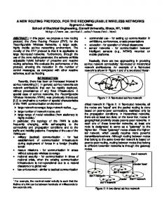
Figure 2.2: Total, announced IPv4 address space since 2008, with a line fitted to the data from 2008 to 1st Feb 2011, showing the effect of IPv4 address space exhaustion. Based on data courtesy of [35]. boom, followed by stagnation in the bust thereafter [38]. There is an apparent return to at least polynomial, and potentially exponential, growth from ’02 onward, which perhaps has been driven by the growth of broadband and mobile devices [38]. There is also an apparent mode change in growth sometime in 2008, indicative perhaps of the effects of the global banking crisis. An additional exponential curve is shown, fitted to just the data from 2009 onward, to reflect this possible mode change. An additional factor that might be expected to affect growth is that the IPv4 address space is in the final stages of exhaustion. IANA made its final allocation on February 3rd, 2011. This was followed by 2 major RIRs, APNIC and RIPE, exhausting their standard allocation pools on the 19th of April 2011 and the 14th of September 2012 respectively [37]. There has been a noticeable slow-down in the growth of the total address space announced via BGP since 2011, presumably due to the exhaustion of those RIRs’ pools, as can be seen in Figure 2.2. There has been no similar slow-down in growth of the advertised IPv4 prefixes, as seen in Figures 2.1 and 2.3. Despite the availability of IPv4 address space clearly now facing significant constraints, the number of distinct IP prefixes being

2.2 Internet Growth

18

500000

450000

# of IPv4 prefixes

400000

350000

300000

250000

200000 Jan 2008

Jan 2009

Jan 2010

Jan 2011 Date

Jan 2012

Jan 2013

Jan 2014

Figure 2.3: BGP IPv4 routing table size, from 2008 to October 2013, with a linear fit over the period from 2008 to 1st Feb 2011, showing continued, fast growth despite adverse global economic conditions and the exhaustion of the IPv4 address space. Based on data courtesy of [35].

2.2 Internet Growth

19

Figure 2.4: IPv4 address space advertised, divided by the number of prefixes advertising that space, over time, to October 13, showing fewer addresses being advertised per routing entry over time. Based on data from [35] where both address space count and prefix count were recorded at the same time. advertised into BGP has continued to increase supra-linearly. This is being achieved at least in part by each of those prefixes covering ever-smaller, de-aggregated, ranges of IP addresses, as can be seen in Figure 2.4. In an ideal world, there would be a graceful transition from IPv4 to IPv6, as explained in [38], which would at least avoid the de-aggregation being seen today. It would not though address the underlying issue of growth in the number of networks attached to the Internet. This graceful transition has not happened, so far. There has so far been little uptake in IPv6 [38], at least relative to the ongoing growth in the IPv4 routing tables. However, the IPv6 tables are also seeing steady and supra-linear growth, as can be seen in Figure 2.5. That growth of the IPv6 routing tables is a concern for the future, even if their current, small sizes are not. Allocations of AS numbers have also seen steady growth, at at least a linear rate or perhaps a low-exponential rate [34]. In summary, the Internet therefore has shown sustained, supra-linear growth, when its size is measured in terms of the size of the BGP IPv4 routing tables. That growth is at least polynomial in scale, but also is not inconsistent with exponential models. That supra-linear growth has continued, despite even the exhaustion of the IPv4 address space. The IPv6 routing tables, though still relatively small in terms of number of entries, are also growing supra-linearly. This growth is creating

2.3 Observed Internet Structure

20

20000

exponential fit polynomial fit exponetial fit (’09 on)

# of IPv6 Prefixes

15000

10000

5000

0

-5000 2003

2005

2007

2009

2011

2013

Date

Figure 2.5: BGP IPv6 routing table growth, based on data from courtesy of [35]. sufficient pressure on router memory and processing power for members of the IETF to have published an informational RFC expressing their concern [52].

2.3

Observed Internet Structure

The structure of the Internet in terms of its connectivity is highly relevant to the efficiency of routing schemes. Some appreciation of that structure is necessary to evaluate any routing schemes that aim to improve the scalability of Internet routing. The Internet is a large, distributed system which has grown over decades according to the varying interests of many thousands of organisations, many of whom further serve or consider the interests of many other organisations and individuals. The resulting graph has edges between at least many thousands of nodes, correlated in quite range of ways, from the objective(s) of the organisations (ISP, content provider, academic institution, etc.), their geographic locations, their ages, their size (geographic spread, financial turnover, etc.), and so on. To illustrate, Figure 2.6 shows the Internet’s connectivity as a sparsity plot of the BGP AS graph adjacency-matrix, with a point plotted where an AS has a link to


21

(a) 200306 BGP AS Graph

(b) 201306 BGP AS Graph

Figure 2.6: Sparsity plot of the adjacency matrix of the BGP AS Graph, based on data from the IRL Topology project [71], restricted to the 16-bit AS space. A point indicates the ASes have an edge.


22

another AS in the matrix, for 2003-06 and 2013-06. The points are coloured by column according to the RIR that assigned the AS, i.e., for any given AS on the x-axis, the vertical points of connections of that AS to other ASes on the y-axis should be the same colour. Starting at an AS on the y-axis and scanning along horizontally, then the colours show the RIR of the AS it connects with on the x-axis. The points are oversized to make them visible at this resolution. As a result one points can overlap on top of and obscure another. The points were plotted in the order of the key, meaning that the 2 major RIRs with the most ASes – ARIN and RIPE – were plotted first, and the smaller RIRs points on top of those. That is, where points are obscured, they obscure things in favour of highlighting connections to the smaller RIRs. Some apparent geographic, size and age correlations are visible. Continuous lines are ASes that connect to most other ASes as , presumably ISPs or content providers. Near-continuous such lines are likely large, global ISPs with customers spread over the globe. Such long-line ASes tend to be more prevalent in lower AS numbers, indicating these tend to be older, well-established ISPs. Shorter lines likely indicate smaller and/or more regional organisations. Geographic correlations are visible as boxes of predominantly the same colour, due to clusters of continuous ranges of AS numbers having been assigned from the same RIR. These colour-dominated boxes suggest ASes from the same RIR tend to connect far more preferentially with ASes from the same RIR (and hence high-level region) than outwith. E.g. the green boxes (and the empty white boxes that correspond to blue boxes above and below) indicate American/ARIN ASes prefer to interconnect with other American/ARIN ASes. These correlations could be interesting to investigate more deeply, in other work. Just from visual inspection, the 2013 graph seems to be an extension of the 2003 graph – the same rough age and geographic correlations appear to have continued on at least. A variety of graph metrics and transformations may be applied to the Internet graph, in order to try characterise it. The degree distribution of the Internet BGP AS Graph generally follows a power-law distribution [22], the slope of which appears to have remained relatively steady over time, as can be seen in Figure 2.7, with the distribution shifting upward as the Internet grows in size. This type of scale-free, power-law degree distribution seen in Figure 2.7 can be modelled via preferential-attachment graph growth [8], in which new nodes are more likely to attach their edges to existing, higher-degree nodes than lower-degree nodes. With this preferential-attachment model of graph growth, each new arriving node tends to further inflate the degree of the highest-degree nodes. So


23

BGP AS Graph Degree Distribution 105

200306 200311 200606 200806 201006 201306 a = 11.06, b = -3.1554, c = 1.1277 a = 11.727, b = -2.9753, c = 3.9466

104

# of nodes with degree

y = ea*xb + c model

103

102

101

100 100

101

102 Degree

103

104

Figure 2.7: Degree distribution of the Internet, over time, with non-linear, least-square fits of a power-law model over a subset of the 200306 and 201306 labelled data-points, as shown. Based on data from the IRL Topology project [71]. preferential-attachment growth results in a graph with a small number of very high-degree nodes, and a long-tail of a large number of much lower-degree nodes. Edges in graphs with such scale-free degree distributions, such as the Internet, tend to be heavily skewed towards there being a high-degree node on at least one side. This is illustrated in Figure 2.8, which shows the proportional, cumulative distribution of the dominant degree of every edge in two AS graphs. For the 200306 AS graph, 95% of edges connect with an AS with a degree of 10 or higher, and 77% of edges connect with an AS with a degree of 100 or higher. For the 201306 AS graph, the figures are 90% for degree 10 or higher, and 60% for degree 100 or higher. This is consistent with the decreased dominance of the power-law component in the 201306 data-set relative to the 200306 data-set, as seen in Figure 2.7. Nodes in a graph can be ranked, such that their rank is determined by a normalised sum of the ranking of their neighbours. This method of ranking nodes called “eigencentrality” and is the basis for the classic, early versions of the Google PageRank algorithm. If this ranking process is carried out in an iterative way, summing neighbour’s ranks and then normalising the ranks at each iteration, the


24

Proportional CDF of the dominant degree of each edge 1 201306 200306

Edges dominated

0.8

0.6

0.4

0.2

0 100

101

102 Degree

103

104

Figure 2.8: Proportional CDF of the dominant degree of each edge in the 200306 and 201306 AS graph data-sets from the UCLA IRL Topology project [71].


25

process will eventually settle on a stable set of rankings for the nodes, such that those rankings are intrinsically determined by the global connectivity in the graph. The rank of a node then depends on its neighbour’s ranks, which each depends on their neighbour’s ranks in turn, and so on. The highest ranking nodes will have higher-ranking and/or more neighbours than lower-ranking nodes, and so on. This ranking corresponds to the eigenvector of the largest eigenvalue of the adjacency matrix. This and related methods in the field of spectral graph analysis can be used for finding clusters and cuts, determining graph-theoretic bounds on certain properties, and characterising graphs. These methods have been applied to analysing the Internet previously [30, 23]. The most immediately accessible application of eigencentrality ranking is perhaps to use it to re-order the rows and columns of the adjacency matrix, such that the rows and columns go from least-ranked nodes to highest-ranked nodes. When plotted in this re-ordered way, some correlations become more apparent. For example, Figure 2.9 reveals the very high density of connections between highly-ranked nodes, while lower-ranking nodes connect to fewer other nodes, which may be characteristic of preferential attachment growth. Further, the more highly-ranked nodes also can be seen to connect to many other nodes, over a wide range of rankings. Strong structural similarities over time are again evident, as seen earlier with the AS-based sparsity plots of Figure 2.6 and in the degree distribution plot of Figure 2.7. Details of the 20 highest eigencentrality-ranked ASes are given in Table 2.1. Unsurprisingly, these are all network service providers of some kind, and all have very high degrees. Somewhat surprising however is that the well-known, large telecommunication company, network providers do not dominate this list, indeed they generally do not feature in it at all. For comparison, Table 2.2 shows the degree and eigencentrality ranking for a number of high-profile Network Service Providers. Note that two of these high-profile NSPs, Level-3 and Centurylink, have their operations divided over at least 2 ASNs. A traditional view of the Internet might focus on the large, telecommunications companies in Table 2.2, who are often thought of as forming the core of the Internet, or on the hierarchy they form. E.g. [30] did so even while aiming to carry out an eigencentrality analysis but deliberately excluded ASes with high eigencentralities which were not deemed to be sufficiently large ISPs, and [67] focused on the hierarchy.


26

(a) 200306

(b) 201306

Figure 2.9: Sparsity plots of the adjacency matrix of the Internet AS graph, with rows and columns sorted by the eigencentrality rank of the AS, based on data from the IRL Topology project [71], restricted to the 16-bit AS space.


Eigencentrality AS Rank 1 AS6939 2 AS9002 3 AS13237 4

AS34288

5 6

AS12859 AS8468

7 8 9 10

AS42708 AS12779 AS13030 AS31500

11

AS28917

12 13

AS12989 AS19151

14 15

AS31133 AS8359

16 17 18 19 20

AS29208 AS8447 AS24482 AS8422 1267

27

Description

Degree

Hurricane Electric RETN Limited euNetworks Managed Services GmbH Public Schools in the Canton of Zug BIT BV, Ede, The Netherlands ENTANET International Limited Portlane Networks AB IT.Gate S.p.A. Init Seven AG,CH JSC GLOBALNET, St. Petersburg, RU. JSC "TRC FIORD", Moscow, RU Eweka Internet Services B.V. Broadband One Announcements, Florida, US. OJSC MegaFon, Moscow, RU. MTS / former CJSC COMSTAR-Direct, Moscow, RU DialTelecom, CZ A1 Telekom Austria AG, SG.GS NetCologne GmbH WIND Telecomunicazioni S.p.A.

2781 1601 1094 1033 912 933 979 962 1101 1151 1083 1198 1007 1141 1217 878 885 858 781 832

Table 2.1: Highest ranked ASes by eigencentrality, out of 41267 ASes with non-0 degree, as visible from the IRL Topology 201306 dataset [71].


Eigencentrality ASN rank 45 AS3356 70 AS174 96 AS1299 99 AS3257 108 AS3549 112 AS3491 115 AS2914 150 AS6461 293 AS3320 307 AS1273 313 AS6453 541 AS6762 750 AS4323 788 AS5400 886 AS2828 924 AS4134 925 AS209 930 AS701 938 AS5511 946 AS15290 951 AS1239 969 AS7018 1142 AS3561

28

Name [/ Other or prior name]

Degree

Level 3 Cogent TeliaSonera Tinet / gtt / Inteliquent Level 3 / Global Crossing PCCW Global NTT US / Verio Abovenet Deutsche Telekom Vodafone / Cable & Wireless Tata Communications / Teleglobe Sparkle / Seabone / Telecom Italia tw telecom British Telecom XO Communications China Telecom Centurylink / QWest Verizon Business / UUNet Orange / OpenTransit Allstream Sprint AT&T Centurylink / Savvis

3949 3909 785 955 1438 616 924 1170 550 315 593 297 1778 196 1101 114 1531 2005 164 189 860 2507 354

Table 2.2: High profile, “Tier-1” and “Tier-2” Network Service Providers, with their degree and eigencentrality ranking, out of 41267 ASes with non-0 degree, as visible in the IRL Topology project [71] 201309 AS Graph data-set. However, by another view such as eigencentrality, there is another world of “smaller”, lower-profile networks, seemingly more regional, building out large webs of connections, and forming their own cores and clusters. These high-eigencentrality, “smaller” networks are building their connections by aggressively peering, likely enabled at least in part through Internet eXchange Points (IXPs), such as AMS-IX, LINX, etc, and particularly in Europe where the IXP model is popular [13]. A majority, 11, of the top-20 Eigencentrality ranked networks in Table 2.1 would seem to be Europe based, and another 6 are in western Russia, whose networks are likely to gravitate toward peering in Europe (the European RIR, RIPE, is the RIR for Russia). These IXPs act as major hubs, however these IXPs are generally not directly visible in the BGP AS graph [5], as they either are not involved in the BGP level connections between those networks, or where they are, the IXPs’ BGP route-server generally operate in a “transparent” mode and do not insert their own

2.4 Unobserved Internet Structure

29

ASN into the AS_PATH. The larger IXPs reportedly carry as much daily traffic between the networks peering at them, as the largest ISPs do over their backbones [2]. These IXPs also enable major content providers to peer directly with many other networks, and there is evidence these major content providers have built out their connectivity widely in this way, rather than relying on the traditional large telecommunications companies to route their traffic for them [29]. The structure of the Internet thus appears to have evolved, as well as our understanding of it. Other studies have also noted the strong correlation between the central cores of the Internet and IXPs with other metrics, e.g. using the k-dense decomposition of the AS graph and noting that all ASes in the inner-most core were at IXPs [31]. Spectral analysis of the Internet AS Graph suggests that the likelihood of nodes with similar degrees being connected (the assortativity co-efficient) has been increasing over time, and that growth in the Internet has shifted somewhat away from consistency with a preferential-attachment model (e.g. with dominant “Tier-1” telecommunications companies) and more toward a flatter, more edge-connected model, with less hierarchy [23]. In short, the Internet is a very complex system. Its modes of growth evolve over time, as organisational needs change. Further still, different structures and modes of growth can dominate in different parts of the Internet due to geographically localised preferences. Any given single measure of the Internet may highlight some of its details, but is certain to miss many others. This thesis will endeavour to embrace those measures for what they are worth, while still being wary of weighting them too much.

2.4

Unobserved Internet Structure

The second major difficulty in characterising the connectivity of the Internet is the empirical difficulty in even accurately measuring or mapping the structure of the Internet, or even representative subsets of it. This means our knowledge of that structure is both incomplete and inaccurate. Two main techniques are used, one being to use traceroutes to probe for connectivity in the forwarding plane of the Internet, the other being to observe BGP announcements and use the “AS_GRAPH” attribute in BGP UPDATE messages. Both methods share the limitation that they are restricted to observing only those edges in the Internet that are contained in the collection of shortest-path trees available from each of their neighbours, at each observation


30

point. The shortest-paths in a graph need not contain all edges in a graph, even if the collection of shortest-paths is complete. Further, these shortest-paths are not drawn from the the full set of edges. Rather the shortest-paths are drawn from a constrained set of edges, with some edges pruned out or their cost modified depending on policy decisions, that may be specific to the path being taken by each BGP announcement. The shortest-path tree at one observation point therefore may be drawn from a very different set of edges to that of another observation point. E.g., networks typically do not announce BGP routes learned via a peer to other peers or to upstream providers, but only to “customers” (i.e. those other networks which it provides transit service to) [67]. So an edge due to such peering between two networks may not be observable to any observation point, other than one located within the customers of those networks – the so-called “customer cone” – or the network itself if it has no customers [19]. To observe all such edges would need observation points within every customer-cone of every network that has peering links to other networks, or the network itself. As another example, some edges may only rarely be on the shortest-path, e.g. because they are expensive, and/or intended deliberately to be kept as backup links. To construct graphs with such edges may require aggregating data over long periods of time. This means there is a trade-off in our measurements with respect to time and the validity of the edges. As a consequence, it should be expected that we have better information on peering links for the larger ISPs with more customers, but that our graphs under-describe connectivity at the edges of the Internet and between smaller networks. This was found to be the case by Oliveira et al. [56], who found the large “Tier-1” ISPs were fully described by public data on BGP connectivity, while smaller “Tier-2” ISPs are relatively well-described, however stub networks and content-providers were poorly described. Further, [56] found that the existing BGP monitors at that time provided good coverage of connectivity for only 4% of ASes on the Internet. In [2], the number of all peering links known from public data for the ASes present at a major IXP was found to under-represent the actual peering links by a factor of more than 3. Indeed, the number of peering links [2] found to be present at this IXP was larger than all known peering links in the Internet. The traceroute observation approach faces further problems. There are a number of practical details that make it difficult to reliably relate a traceroute observation to an actual edge in Internet connectivity. Traceroutes consist of a sequence of packets sent with TTLs set in ascending order, so as to solicit the return of ICMP “TTL Exceeded” messages from routers along the forwarding path. However, the router returning the message may have a number of IP addresses, and the address it sets in the ICMP message need correspond to neither the link the ICMP


31

message is sent on, nor to the link on which the packet that provoked the ICMP message was received on. Alternatively, the router may re-use IP addresses across multiple links, and so the address may be insufficient to distinguish between them. This is assuming the router even sends an ICMP message or, if it does, that the ICMP message is safely received by the probing traceroute host. Further, even if those obstacles are overcome, and router-level edges can be determined, it still can be difficult to relate those edges to other entities such as organisations, as represented by AS numbers. The organisation which the IP address in the ICMP message is assigned to need not correlate with the organisation that operates the router, e.g., it may have been assigned by the other party on that link. The IP address assignment is not even guaranteed to correspond to the organisations running either of the routers on each side of the link, as it may actually belong to a 3rd party providing a shared-fabric (e.g. an IXP or a data-centre operator). This can lead to organisational level edges being missed, and other, spurious edges being inferred. E.g. A-B-C may be inferred as A-B, if the messages from C are not present in the data, or if the message(s) from C have addresses from A or B. As a result, constructing connectivity graphs from traceroute data can be error-prone. E.g., between 14% to 47% of edges in AS-graph connectivity constructed from well-known public traceroute data sets are likely incorrect, according to [72]. Heuristics can be applied to try address these problems, and attempt to detect spurious edges and compensate and/or filter them out, as in [14], which used traceroute data collected from an extension in a BitTorrent P2P client to construct an AS graphs. The filtering heuristics of edges were further validated against ground-truth of a Tier-1 AS, and found to have correctly removed all false links, at least for that AS. Based on this, they found 13% more customer-provider links and 41% more peering links than were previously known to exist in the Internet. An additional problem with AS graphs is that the AS_PATH attribute in the BGP messages may contain almost anything. The AS_PATH usually describes ASes the message has traversed, thus allowing edges of the AS graph to be inferred. However, nothing stops BGP speakers modifying the AS_PATH, be it to remove ASNs or to add additional ones. BGP speakers may modify the AS_PATH for a variety of reasons. A BGP speaker may wish to deliberately hide some ASNs, e.g. customers without global AS numbers but using private ASNs, or to hide a business relationship. A BGP speaker may deliberately insert ASNs it has no actual connection with, e.g. for traffic engineering purposes so as to prevent an advertised route reaching/traversing certain other ASes, for nefarious purposes in order to “Man in the middle” traffic to another AS [33], or for experimental

2.5 Routing Table Scalability

32

reasons where researchers are trying to probe and measure the working of Internet BGP (e.g. as in [11]). In short, there are significant practical challenges to measuring the structure and connectivity of the Internet. These challenges mean our knowledge of that structure is incomplete and its connectivity is under-described, particularly at the edges. While our view of the actual network structure is incomplete, the view we do have can contain additional, spurious, “junk” edges. This will impact on any evaluation of proposed improvements to Internet routing. Such evaluations will have to be aware of that incompleteness and uncertainty.

2.5

Routing Table Scalability

A simple universal shortest-path routing scheme is to have each of the N number of nodes in a network maintain a routing table with an entry for the shortest-path to every other node. The per-node memory requirements for these tables scales no worse than O (N log N ), as each node can obviously can be differentiated with O (log N ) labels (i.e. addresses), and each node stores O (N ) vectors composed of some constant number of fields subject to the bound on the label, e.g. the destination label and an output port. Such shortest-path routing tables grow supra-linearly as the network grows with nodes, in the worst case [45, 27]. Further, any universal shortest-path routing scheme for arbitrary graphs will use at least Ω (N 2 log ∆) routing state summed across all nodes, where ∆ is the maximum degree in the network [27]. This implies routing state locally at each node requires Θ (N log ∆), i.e. intuitively the per-node memory requirements must more or less average out to this. Hence, no universal shortest-path routing scheme can exist that can scale sub-linearly. It may be that shortest-path schemes could be designed to be compact on specific classes of networks, however no such scheme can be compact universally on all networks. The proof of Gavoille and Pérennès [27] proceeds by characterising the shortest-paths in graphs (which any shortest-path scheme must be capable of relating to in some way) as matrices of constraints on graphs. In characterising the memory required to describe the shortest-path constraint matrices, the paper argues this then must also describe the minimum memory requirements of any shortest-path routing function. The paper then goes on to describe bounded systems of constructions of shortest-path constraints and their graphs, from which follows the bounded memory requirements on the size of shortest-path routing schemes.


33

Such supra-linear scaling means that the memory in each node must grow as the network grows so as to be able to hold this routing state. Increased routing state may imply increased communication between nodes, if they must synchronise this extra state. All this may happen even as the network immediately around the node stays unchanged. Adding new nodes to the network then may require having to add hardware to all nodes, as Awerbuch et al. [7] put it. This supra-linear scaling of the routing tables in each node may become infeasibly expensive as a system becomes large – the Internet possibly may be such a system. In such cases, having the routing tables scale sub-linearly as the network grows would be desirable[52]. Routing schemes with such sub-linear scaling of per-node routing state in the worst-case (i.e. “compact state”), and where the node label or address are bounded logarithmically, are known as “compact routing schemes”. As sub-linear scaling can not be achieved with guaranteed shortest-path routing, achieving this requires conceding that at least some routes between nodes may be longer than the shortest-path – they are “stretched”. That is, some amount of shortest path routing must be traded away to gain state scalability and compactness of routing tables. This stretch can be quantified as either multiplicative (the ratio of the actual path length to the shortest path length) or additive (the number of extra hops taken, relative to the shortest path). Stretch can be given for specific nodes, for the best or worst cases in a scheme, or the average of a scheme. Some papers have used an (α, β) Figure 2.10: A (3/2, 1)-stretch notation for stretch, where α is the multiplicative path, shown in red. stretch, and β the additive stretch of a path or routing scheme, such as in Thorup and Zwick [68]. Generally it is the worst-case, multiplicative stretch of a routing scheme that is the most interesting measure and so that is what is meant here when talking about the “stretch” of some routing scheme, unless specifically stated otherwise. Initial attempts at reducing routing stable state sought to group nodes together, into a hierarchy of clusters. The hierarchy forms a tree, and the clusters and nodes are typically labelled in accordance with it. The clusters can be used to abstract away the nodes within them. The routing tables then need only store shortest-path vectors for nodes within the same lowest-level cluster, and for a limited set of all the other clusters, such as sibling clusters in the hierarchy. This hierarchical routing potentially allows a great number of routing entries to be eliminated, particularly when the depth of the hierarchy is logarithmic in the size of the


34

Figure 2.11: Compact routing bounds and results network – though, of course, at the expense of non-shortest-path routing. In Kleinrock and Kamoun [43] it was shown that in the limit of network growth, the average stretch of hierarchical routing schemes becomes insignificant, while the routing table savings can be very significant. This result depends on the diameter of the network growing along with the size of the network, something which need not happen with any significance with small-world networks like the Internet[50]. Hierarchical routing is examined in further detail below, in Section 2.7. Insignificant average stretch unfortunately still allows for very bad worst-case stretch. A routing scheme with high or unbounded worst-case stretch may never be practical, even if it leads to compact tables. Trivial average stretch may be of no comfort to nodes forced to communicate over highly-stretched paths. This may even lead some nodes, if the routing scheme allows it, to over-ride the scheme in some way to add back routing state to reduce the worst-case stretch, undoing the state scaling benefits of the scheme! This led to the development of compact routing schemes whose worst-case stretch (simply referred to as stretch from here-on) is bounded by a constant. Gavoille and Gengler [26] showed that schemes with a stretch below 3 can, in the best case, achieve only linearly-scaling growth in routing table state. Thus, any compact routing scheme must have a stretch of 3 or greater. More generally, Peleg and Upfal [59] showed that any general routing scheme with a stretch factor of k ≥ 1 must use at least Ω N 1+1/(2k+4) amount of state over the sum of all nodes.

2.6 Degree Compact

35

Cowen [17] described a stretch-3 compact routing scheme based upon categorising a subset of nodes as “landmarks”, using an extended dominating set algorithm – Cowen Landmark Routing. All other nodes are associated with their nearest landmark, and their labels are prefixed with their landmark’s identity. All nodes maintain shortest-path routes to all landmarks. Additionally, non-landmark nodes maintain a local routing table, with shortest-path vectors to those nodes “near” to them, according to their respective distances from their landmark. This scheme √ ˜ 3 N 2 routing table scaling1 . With a modification to the landmark achieves O selection scheme to use a random selection, [68] showed Cowen Landmark Routing √ ˜ per-node state could scale with O N . The details of Cowen Landmark Routing are examined further below, in Section 2.8. These results are summarised in Figure 2.11. A useful summary is also given in Krioukov et al. [45]. The interesting problem is to try take any of the theoretical routing schemes in the compact region and which have bounded worst-case stretch, and determine what obstacles there are in turning them into practical, deployable, distributed routing protocols and then try overcome those obstacles.

2.6

Degree Compact

The theoretical definition of compact routing requires compact state at all nodes, in any graph. This means that even on graphs where some node’s degree increases in the same order as the rate the network increases in size, i.e. at Θ (N ), a routing scheme must still produce sub-linear, compact state at that node to be considered a compact routing scheme. A graph with nodes which have Θ (N ) degrees must be one where new nodes attach to a fixed number of central nodes, distributed in a fixed proportion, i.e. a hub and spoke graph. Practical network protocols often retain some state for all neighbours. This would mean their state strictly speaking could not be described as “compact” according to the accepted theoretical definition, even if all other state retained by the protocol at each node is still no worse than sub-linear with N . Instead, let these protocols be referred to as “degree compact”. Practical networks however always have ways to avoid Θ (N ) degree scaling, if they wish. In practical networks, administrators can choose whether to create new links and simply refuse to bring up new links if the new link would over-burden available resources. Alternatively, if new links must be brought up, but the neighbour state at a node is becoming onerous, the administrator can add more nodes and scale ˜ (f (n)) is shorthand for O f (n) logk f (n) , discarding the logarithmic factor, as f (n) will O ultimately dominate the bound. 1

2.7 Hierarchical Routing

36

the load out. Administrators can add routers to their network, and can divide up an AS into confederations or entirely new subsidiary ASes, as required. Consequently, this dissertation will consider degree-compact protocols to be equivalent to compact protocols, for all practical purposes.

2.7

Hierarchical Routing

Hierarchical routing is the basis for widely used routing protocols today. The areas of OSPF and the levels in IS-IS are examples of hierarchical routing. Even the BGP routing of the Internet, which appears on the face of it to result in pure shortest-path routing tables, is a form of hierarchical routing, as the shortest-path routes are between IP prefixes which may cover large groups of nodes. Thus the Internet already is using a routing scheme with the potential to be compact, though with unbounded stretch. The efficiency of hierarchical routing depends on two factors. Firstly, in order to achieve compact routing, a hierarchy must be found in the network or imposed on it – there must be some way to cluster the nodes. Secondly, in order to minimise stretch, that hierarchy must align well with the connectivity of the network. While it is generally possible to impose a hierarchy on most kinds of networks, and so it is nearly always possible to achieve compact routing tables, it may be difficult to optimally align that hierarchy with the connectivity. Though, that hierarchy does not need to be deep to achieve significant benefits in state reduction [43]. However, well-connected, small-world networks, where the network diameter does not increase significantly with network growth[50], such as the Internet, may suffer from larger degrees of average stretch with hierarchical routing than otherwise. E.g., Krioukov et al. [44] estimated that the scheme of Kleinrock and Kamoun [43] would result in average stretch increasing with the network size according to log2 N s ∼ log on scale-free graphs, with an average stretch of around 15 on log N Internet-like graphs. An average stretch of 15 does not compare well with the worst-case stretch of 3 achievable with Cowen Routing, which will be introduced later in Section 2.8. To understand how to improve on hierarchical routing, its strengths and weaknesses need to be understood first. Hierarchical routing is based on the principle of clustering together nodes that are “near” each other in the network, and clustering the clusters similarly, such that the clusters form a hierarchical tree. The nodes are then given labels according to this tree some way, such that these labels allow cluster memberships to be deduced or found. In the simplest case the


37

label is structured so that it contains cluster identifiers prepended to each other, giving the precise location in the hierarchy of a node. In more complex schemes, knowledge of the location of the label is distributed over the network in some systematic way. Regardless, each level of clusters reduces the state needed to route to that cluster by others, and the routing of messages then follows the hierarchy.

Figure 2.12: Clustering of nodes into a hierarchy. Destination 15 16 17 C D

Next-Hop 15,16 4 13

Hops 1 1 2 1 1

Table 2.3: Example hierarchical routing table for Node 14 of Figure 2.12 As an example, Figure 2.12 shows a network and a possible clustering of those nodes. A possible hierarchical routing scheme, such as that of Kleinrock and Kamoun [43], might have node 14 labelled as “A.B.14”. Node 14 would store shortest-path routes to its sibling nodes in cluster B, and to the sibling clusters of each of its parents clusters – that is, cluster C as the sibling of B, and cluster D as the sibling of A. The resulting routing table for node 14 is given in Table 2.3. The routing table is significantly more compact, with only 5 entries, than it would be with a full shortest-path routing scheme, which might potentially require 16. However, this obviously must come at the cost of stretched paths. E.g., node 14’s shortest-path to cluster D happens to enter D at an extremal point of cluster D. As a result most paths from node 14 to nodes within cluster D are quite stretched, particularly to any nodes in cluster E. The path from node 14 to node 7 is 4 hops, rather than 2. This is as node 14 will never use node 4 to route toward cluster D, as node 14’s own link to cluster D will always have a lower cost.


38

As another example, while node 14 generally has stretch-1 paths to nodes in cluster C, the path to node 1 is stretched a little by 4:3. This could be avoided by placing node 1 into cluster B instead, however this would just lead to additional stretch on other paths between other nodes. Further, if the connectivity between the nodes in cluster D and A, other than node 14, were to increase then this could actually increase the stretch of paths from node 14 to nodes in cluster D. That is, increased connectivity could decrease the length of shortest-paths between node 14 and nodes in D, e.g. if there was a link added between nodes 9 and 15. However as those shorter paths simply will not be used by node 14 then it means the stretch from node 14 will actually increase. The preference for nodes in a hierarchical routing scheme to use the shortest-path to the boundary of a cluster, regardless of the costs from that boundary to the destination inside the cluster, is referred to as “Closest Entry Routing” in [43]. It is also often known as “hot potato routing”. It would also be possible to assign costs to inter-cluster edges, to reflect the suitability of the node the edge is incident on for routing into that cluster. E.g., if the node is more central to the cluster, it could have a lower cost than other nodes. This is called “Overall Best Routing” in [43]. This could help optimise the average stretch, but can not eliminate it. Hierarchical routing provides universal, compact, routing with good average stretch on at least some networks. Indeed, Kleinrock and Kamoun [43] showed average stretch can diminish to insignificance on many networks with hierarchical routing as they grow. However, hierarchical routing schemes generally did not specify how to efficiently construct a hierarchy in a way that guaranteed acceptable reduction in routing state, and/or that achieved minimal average stretch. E.g., Kleinrock and Kamoun [43] left the choice of hierarchy as a case-by-case optimisation problem; Peleg and Upfal [59] specified a centralised, polynomial-time construction, and gave a guarantee of overall state being compact in the worst-case but did not make that guarantee per-node; and so on. Further, the problem of worst-case stretch was often left open. Worst-case stretch is intrinsically unbounded in hierarchical routing. The very tool hierarchical routing uses to provide compact state, of abstracting away nodes by encapsulating them in clusters, also abstracts and hides information about the connectivity within a cluster to all those outside it. The hierarchy of clusters not only abstracts routing state, but imposes itself in such a way that the messages must follow the hierarchy. So two relatively nearby nodes might end up in clusters that are connected via a relatively distant link between parent clusters, and messages between might have to travel a long way up and down the hierarchy, for want of local knowledge about a better link.

2.8 Cowen Landmark Routing

39

In practical networking, such as with BGP on the Internet, network administrators may choose to work-around such undue stretch in hierarchical routing by effectively breaking out of the hierarchy. Administrators may choose to globally advertise additional “more specific” routes, for the locations that do not fit well into the hierarchy. Or they may, somewhat equivalently, simply choose not to cluster together different locations into one advertised routing prefix, but advertise each separately. This “traffic engineering” may improve the connectivity to the networks concerned by reducing the stretch, but does at the cost of additional routing entries at all routers. Awerbuch et al. [7] attempted to address some of these issues. It specified a greedy, graph-cover based method for selecting a hierarchy of “pivots” or “centres” around which nodes are clustered. The stretch of the scheme was bounded. However, the bound on the stretch was inversely and polynomially related to the per-node state bound, with O k 2 3k stretch versus O kn2/k log n per-node state, for a hierarchy of k ≥ 1 levels. This implies both that the stretch in the scheme grows quickly as the number of levels increases, and that at least 3 levels are required to guarantee a modest, compact bound on per-node routing state. Though this scheme does not deliver compact routing for a fixed bound on stretch, it did manage to put a bound on worst-case stretch. This scheme is also interesting for containing concepts that will be seen again in Cowen’s Landmark Routing scheme, described below in Section 2.8. Such as selecting certain nodes using a graph cover algorithm to cluster other nodes around, and taking the size (number of member nodes) into account when constructing clusters. The scheme is described by the paper itself as being quite complex, in at least some aspects of how packets are forwarded. The problems left open by the early work in compact routing were to find a scheme meeting all the following criteria together: • The bounding of worst-case stretch to a reasonably low and fixed constant • The compact bounding of per-node state • The efficient selection of a routing hierarchy

2.8

Cowen Landmark Routing

Cowen [17] answered some of the questions posed by the earlier hierarchical routing work. Her Cowen Landmark Routing scheme provides significantly √ √ ˜ 3 N 2 , or even O ˜ compact, per-node routing state, potentially down to O N


40

with a modification, while also guaranteeing stretch would be no worse than a factor of 3. It did so using a 2-level hierarchy which divides nodes into “landmarks” and other nodes, but crucially allowing routing information to be better distributed locally than in traditional hierarchical schemes. These landmarks are selected purely in accordance with properties of the graph – no external metric space or geographical knowledge is involved. Moreover, the scheme has a simple message routing process, and even the proofs are straight-forward. While Cowen had specified a particular method for selecting those landmarks, her proofs in [17] for the state and stretch bounds can apply generally to any landmark selection process meeting certain coverage criteria. The overall bound is composed of the sum of a bound on the landmark set size, and a bound on the cluster sizes, with relatively few dependencies between the two in their proofs. Hence, those proofs are easily decomposable, and so can act as a framework even if the landmark selection process is changed significantly, as evidenced by [68], described below . This gives the scheme great power. Cowen used the same greedy graph cover algorithm as in [7] for landmark selection √ ˜ 3 N 2 result. Thorup and Zwick [68] built on that work and to obtain the O demonstrated a compact routing scheme with an even tighter bound on its state, √ ˜ at O N , by modifying the landmark selection to use a random selection process. These results place the Cowen Landmark Routing scheme firmly in the compact state region of Figure 2.11. The Cowen Landmark Routing scheme works by distinguishing between routing to “near” and “far” nodes, at each node in the graph. A sub-set of the nodes are chosen to be “landmarks”, such that every non-landmark node has at least one landmark near to it. All nodes and landmarks store shortest-path routes for all landmarks. Additionally, nodes keep full shortest-path routing tables for a subset of those near nodes – its local cluster. Routing to any far away node can then be done by directing the message toward its landmark, which can be determined from its label. A key contribution the Cowen Landmark Routing scheme makes is that the scope of routing to “near” nodes is determined in a topographically sensitive manner, by reference to the distances from each node to the landmarks. With the landmarks themselves also chosen in a topographically sensitive manner. Non-landmark nodes have their labels prefixed with the label of their nearest landmark, and the index of the shortest-path vector from the landmark to the node. However, the landmark could also store shortest path routes for those nodes within its boundary, it’s own local cluster, without affecting the compactness of the scheme, if there is some other mechanism to ensure the landmark’s local


41

Figure 2.13: Cowen Landmark routing cluster is bounded in the same way as for non-landmark nodes. In which case, the labels would consist only of the landmark’s label prefixed to the destination node’s label. This section will assume such a mechanism exists from here on, such as the mechanism given later in Section 5.4, rather than using the “landmark output port label” approach of the Cowen scheme. As an example, Figure 2.13 shows a subset of a graph, with landmarks highlighted, and with the boundaries of nodes’ closest landmarks shown. The clusters of nodes A, B and D are also shown, with all other clusters omitted for clarity. Note that node clusters are distinct from the closest-landmark boundaries and may overlap, and the cluster condition may result in quite a variety of cluster shapes and sizes. Routing to “far” nodes initially proceeds by following the shortest-path to the remote node’s landmark, shown by green arrows for a selected few cases. Whether the packet actually goes through the landmark depends. The packet may, as it gets closer to its destination, reach a node which has the actual destination in its “near” cluster before reaching the landmark, in which case that node must have a shortest-path to the end-node and will use that instead, shown by the orange arrows. In the worst case, the packet reaches the landmark of the destination, and is then routed along the shortest-path from the landmark to the destination, shown with a red arrow. E.g., if A attempts to communicate with C (which would be labelled L1:C), it


42

sends a packet addressed to L1:C towards landmark L1, which A stores a shortest path for. B might have C in its cluster in which case B will direct the packet straight to C – the packet does not traverse L1. The resulting route also happens to still be shortest-path. Note that even when a packet does traverse a landmark, the route taken may still be shortest-path. E.g. D does not have a shortest-path to E, so sends any packet for E to its landmark L2, and L2 directs the packet on to E. However, it just happens that this path is also the shortest-path from D to E. Other paths may have stretch, e.g. D to F has a stretch from 3 hops to 4. The idea behind the general proof in [17] is to construct each node’s local routing cluster and select the landmarks in such a way as to balance the size of nodes’ local clusters with the total number of landmarks, that it results both in the landmark set size and the size of any node’s local cluster size each being bounded by O N k log N , for k < 1. The per-node routing state then is the sum of those ˜ N k . If that balance is bounds, multiplied by the O (log N ) label size, which is O met, then the scheme is always sub-linear – i.e., compact – in its per-node routing state requirements. In [17] the balance between the landmark set size and the cluster sizes depends on an α parameter, where 0 ≤ α ≤ 1, such that the first N α nearest neighbours (tie-break by label) of a node are defined as its ball. The local cluster of each node is potentially a subset of that ball. The set of landmarks are seeded from a set of covers such that every non-landmark node has at least one such landmark-seed in its ball, and so the landmark-seed set forms a cover over the set of balls. This initial landmark set is augmented by adding to it any nodes which lie in more than 1+α N 2 such balls. Using the greedy algorithm given in [7] to determine the covers, 1+α the final landmark set is no larger than O N 1−α log N + N 2 , and the resulting

local routing clusters are no larger than O N h

1−α

O N log N + N √ ˜ 3 N2 . O

1+α 2

i

1+α 2

, which gives an

log N scheme. Choosing α = 1/3 +

2 log log N 3 log N

gives

Using a randomised, recursive landmark selection process, Thorup and Zwick [68] √ ˜ were able to tighten this result and obtain an O N routing scheme, using the general framework of [17]. Their landmark selection process uses a parameter s, with 1 ≤ s ≤ N , to randomly select a sub-set of nodes to act as landmarks. It does so by iteratively taking the set, W , of the remaining, non-landmark nodes and selecting a random sub-set of W to add to the landmark set, where each node has a s/|W | probability of being selected. At each iteration it computes the resulting clusters, and it repeats the selection process on all those nodes whose clusters are larger than 4N/s, until no such nodes remain. The result is that the selected √ landmark set is no greater than 2 N log N and no cluster is larger than


43

Figure 2.14: Cluster geometries in the Cowen scheme for a select few nodes, in some subset of a network, where the larger, outlined nodes on the left and right are landmarks; and the smaller, solid nodes are ordinary nodes. Distances to the nearest landmark are shown by the arcs. √ 4 N log N . Adding together and multiplying by the label bound gives the √ √ ˜ O N bound on per-node state. This is very close to the Ω N lower-bound for stretch-3 routing found by Krioukov et al. [45]. The local routing cluster of each node is defined through a cluster condition. In the original Cowen scheme of [17] the cluster condition selects those remote nodes which are which are nearer to the node at hand, than the remote node is to its own landmark. Figure 2.14 illustrates the clusters for a select few nodes, in a subset of a network. Note that neighbours need not be in the local cluster, and that the routing cluster tends to extend away from the landmark. Precise routing information on nodes that are closer to their landmark than the local node is sacrificed to gain routing scalability, in the knowledge that this will not harm forwarding efficiency greatly, as will be explained below. Thus, for any node n, if another node m is not in the local routing cluster of n it must be that either m is a landmark, or m is closer to its landmark than it is to n.


44

This cluster condition gives rise to an important constraint, which must always be met in order to guarantee that all nodes are reachable from every other node: Cowen Landmark-Forwarding Constraint: For a node n, associated with a landmark l, every node m on the best path from l to n must have n in its local cluster. Put another way, a node may only associate with a landmark if there is also a routable path from the landmark to it. If there were some m between l and n which did not have n in its local cluster, then it would try to route the packet for n via l, but l would route the packet via m, which would lead to a loop. Note that this does not imply that n must have every m in its cluster. The cluster condition guarantees that the stretch is always bounded to 3, when a remote node v is not in the local shortest-path routing cluster of a node u. The proof is beautifully simple. Say S is the length of the shortest path from u to v, L the length from u to L (v) the landmark of v, and V from the landmark of v to v, as in Figure 2.15. Figure 2.15: Triangle Proof If messages from u to v must forward through v’s landmark then the route taken will be of length L + V in the worst case. By the triangle inequality L ≤ S + V , which by adding V means that L + V ≤ S + 2V . As v is not in the cluster of u, the cluster condition implies V ≤ S. Which implies L + V ≤ 3S, meaning the worst-case path length can have a stretch no worse than 3. Note that even when a packet must be forwarded towards the landmark of a destination it may still follow a shortest-path. This can happen where the shortest-path to the destination is simply an extension of the shortest-path from the source to the landmark, as with the path from node D to E in Figure 2.13. This may also happen when, along the shortest-path to the landmark, there is a node which is on the shortest-path to the destination and has the destination in its cluster, as is the case with the path from A to C in Figure 2.13 – the message forwarding can then “short-circuit” and avoid taking the round-about path via the landmark. Even if a short-circuit of the landmark does not result in the shortest-path being taken, e.g. because the node at which a message is first re-routed according to the local clusters does not lie on the shortest-path, the worst-case stretch is still avoided by not having had to proceed all the way to the landmark.


45

It is this ability for nodes along the way to short-circuit routing via the landmarks, because of the local cluster routing tables of each node, which distinguishes Cowen Landmark Routing from hierarchical routing. In hierarchical routing each level in the hierarchy of clusters fully abstracts the nodes enclosed in the cluster, and thus demands that the routing follow that Figure 2.16: Path which hierarchy, which introduces potentially great stretch. short-circuits the landmark Cowen Landmark Routing takes a more flexible approach, allowing routing information to still “bleed” out locally around nodes in a carefully controlled way. This allows Cowen Landmark Routing to avoid some of the problems of hierarchical routing, and provide a guaranteed bound on stretch. Further, the average stretch of Cowen Landmark Routing can be very good, particularly on scale-free, small-world graphs. Krioukov et al. [44] investigated the average-stretch of the Thorup-Zwick variant of Cowen Landmark Routing on such scale-free graphs and obtained results analytically for a certain scale-free graph model, as well as results for generated scale-free graphs. Their analytical results found that 58.7% of paths were shortest-path (stretch of 1, i.e. no stretch), while 94.45% of paths had a stretch of 3/2 or less. Their generated graph results found 70.8% of paths were shortest-path, and 95.94% were stretch-3/2. Further, in both the analytical and generated cases, the number of paths with a stretch of 2 or greater were insignificant, at 0.434% and 0.210% respectively. Strowes and Perkins [66] observed similarly minimal levels of stretch on graphs obtained from observations of Internet BGP updates. Strowes and Perkins [66] found a mean stretch of circa 1.1, that 75.1% of paths were stretch-1, that 90% of all paths were stretch 0 do 3: Gk ← G 4: while (I ← {v ∈ G : |Ndeg (v, k)| < k}) 6= ∅ do 5: G←G\I 6: end while 7: k ←k+1 8: end while before (i.e. I = H 0 \ H), Relation 4.2 may also hold for some, however it can not hold for all, otherwise at least one k-core in H would not be a maximal sub-graph, contradicting its definition. Thus for any H 0 , either there is at least one vertex that is inconsistent with Relation 4.2, or it must be that all vertices are consistent and so H 0 = H. Thus, if I is not the empty-set this implies there must exist a vertex in H 0 that is not consistent with Relation 4.2, and vice versa: I 6= ∅ ⇔ ∃w ∈ H 0 : |Ndeg (H 0 , w, k)| < k

(4.3)

Removing any such inconsistent vertices, I, from H 0 , successively if required, until all remaining vertices satisfy Relation 4.2 must then obtain the k-core H again. Implication 4.3 means I can equivalently be defined without any knowledge of the actual k-cores, H, through this repeated removal of vertices that do not meet Relation 4.2. Having H 0 , and being able to determine I, implies then being able to determine the k-core H. This process leads to Algorithm 4.1. Algorithm 4.1 starts by assigning all vertices, including any disconnected vertices, to the 0th -core. It then repeatedly removes all 0-degree vertices (and their edges) from the graph until no more such vertices remain; the remaining vertices form the 1-core; then all 1-degree vertices are repeatedly removed; and so on, until there no longer are any vertices left to assign to further cores, and all k-cores for all k are known. If Algorithm 4.1 is evaluated in a purely sequential manner, vertex by vertex, then the number of those evaluations is lower-bounded by Ω max (kmax)2 , where max (kmax) is the value of the highest k-core1 . This is because the outer-loop must run at least max (kmax) times, iterating over each k-core from k = 1 to k = max (kmax), and in each such outer-loop there is an inner-loop which must examine at least k vertices. Accordingly, in total Pk=max(kmax) 1/2 max (kmax)2 + max (kmax) vertices must be examined, at a k = k=1 1

This terminology may seem slightly awkward. It is chosen for consistency with terminology in the context of the distributed protocol, to be introduced later.

4.2 Towards a Neighbour-local k-Core Algorithm

62

minimum, in the absolute best case. The checking of vertices for inconsistency in the conditional of each iteration of the inner loop of Algorithm 4.1 could potentially be parallelised, so that every vertex in the k-core being considered in a given iteration could be evaluated together. Though, the inner loop itself would have to remain. If the vertex consistency checking was parallelised, then Algorithm 4.1 would still require at least Ω (max (kmax)) evaluations. Note that while it’s conceivable that the vertex consistency checks within the conditional of the inner loop of Algorithm 4.1 could be parallelised, the outer loop can not be parallelised. In the inner loop, the consistency of a vertex in any given iteration can be checked independently of the other vertices, and so there is potential for parallelisation in the inner loop. For the outer loop, each iteration depends on the previous iteration having been completed. This data dependency means the outer loop can not be parallelised.

4.2

Towards a Neighbour-local k-Core Algorithm

Algorithm 4.1 acts on the full state of the graph, and requires various intermediate graphs to be calculated, making it difficult to implement efficiently in a distributed manner. To construct an efficient, distributed algorithm for the k-core graph decomposition, the membership of any vertex in any k-core must be expressed solely in terms of its neighbours, and free of any dependency on knowledge of any greater sub-graph. The following will show how this can be done, first presenting a mutually recursive definition, then introducing constraints that allow the k-core membership to be bounded in a such a way that all k-core memberships can be calculated. First note that, as the k-cores are nested, so the highest k for which a vertex is a member of a k-core in a graph G is sufficient to determine all the k-cores which the vertex is a member of in G. Define the highest k membership of a vertex v to be kmax(v), and let Nkmax (v, i) select those neighbours w of a vertex v with a kmax(w) of at least i, in a similar fashion to Ndeg (v, i), so that Nkmax (v, i) = {w ∈ N (v) : kmax(w) ≥ i}. The goal then is to determine kmax(v) for each vertex v in an arbitrary graph G in an efficient, distributed manner. Finding a solvable expression for kmax(v) at each vertex that uses information only from the immediate neighbours of a vertex would then provide a basis for a distributed algorithm. Recall that membership of a k-core is defined by having at least k neighbours in


63

that k-core. Finding maximum values for Relation 4.2 by examining each of the neighbours of a vertex v ∈ G and determining the largest number i such that at least that many of its neighbours w ∈ N(v) have a kmax(w) of at least i, gives a direct equivalence for the kmax(v) of each vertex v: kmax(v) = max {i ≤ |Nkmax (v, i)|}

(4.4)

This equivalence of Equation 4.4 meets the objective of being dependent only on neighbour-state. However it is not solvable for any vertex v as this expression for the value of kmax(v) depends on Nkmax (v, i) which in turn depends on the kmax(w) of each of the neighbouring vertices of v, w ∈ N(v), each of which of those neighbours in turn depend on kmax(v). Hence the equivalence of Equation 4.4 for kmax(v) is a circular definition which does not provide any starting point from which to calculate kmax(v) for any vertex v. To find a form that is solvable, note that kmax(v) ≤ deg(v), for all v ∈ G. This implies the degree of a vertex in the full graph provides an initial bound on kmax(v). If this upper-bound is used as a starting point and this starting point is fed-back, then this gives a process which obtains ever tighter bounds on kmax(v):

kbound (v, t) =

  deg(v)

if t=0

 max {i

≤ |Nbound (v, i, t−1)|} if t>0

(4.5)

Where t ≥ 0, and Nbound (v, i, t) is used to select the subset of a vertex’s neighbours, w ∈ N(v), whose kbound (w, t) is at least i in a similar fashion to Nkmax (v, i) and Ndeg (v, i): Nbound (v, i, t) = {w ∈ N (v) : kbound (w, t) ≥ i} As shown below in Subsection 4.2.1, kbound (v, t) must converge on kmax(v) as t increases. That is, there must exist some value for t ≥ 0, so that kmax(v) = kbound (v, t), for all v ∈ G. Thus, Equation 4.5 gives a solvable form for kmax(v). Compared to Algorithm 4.1, the kbound (v, t) of Equation 4.5 does not need knowledge of the full graph at any stage at any vertex. Further, as the value which kbound (v, t) is converging on is kmax(v) this means that kbound (v, t) is testing for all possible k-cores that v is a member of – not just some specific, a priori, given


64

k-core.

4.2.1

Convergence on kmax(v)

Intuitively, the guaranteed convergence of kbound (v, t) to kmax(v) may be seen by noting that its value describes membership of a number of possible k-core sub-graphs. Then kbound (v, t) applies tests similar to Relation 4.2 and Implication 4.3 for some number of these sub-graphs at once, checking if the memberships are consistent. Vertices whose membership is not consistent lower their value, removing themselves from membership of higher k-cores. This process repeats, until all vertices are consistent. Thus, that the full-graph Algorithm 4.1 converges on the desired k-core means that kbound (v, t) converges on kmax(v) for each vertex v, given that kbound (v, 0) has assigned each vertex memberships of all the k-cores that may initially be plausible. This intuitive sense of the convergence of kbound (v, t) on kmax(v) for each vertex can be proven according to the following outline: 1. Each vertex starts with its kbound (v, 0) greater than or equal to its maximal k-core. 2. The kbound (v, t) calculated at each vertex can only decrease as t increases. 3. If the kbound (v, t) at any vertex is greater than the maximal k-core of that vertex there must be a vertex whose kbound (v, t) will change for t+1. 4. If for each vertex v the kbound (v, t−1) is greater than or equal to the respective maximal k-core, then no vertex can calculate a kbound (v, t) lower than its maximal k-core. The formal proof of which now follows. First starting with a number of preliminary definitions. Definition 4.1. A vertex v is consistent at t iff kbound (v, t+1) = kbound (v, t). Definition 4.2. When all vertices are consistent at t, each with their value of kbound (v, t), then the graph is in a satisfying state. The set of these values, {kbound (v, t) : v ∈ G}, are the satisfying values. Lemma 4.3. For every v ∈ G, kbound (v, 0) ≥ kmax(v). Proof. This follows as kbound (v, 0) is defined to be deg(v), and deg(v) ≥ kmax(v).


65

Lemma 4.4. kbound (v, t) ≥ kbound (v, t+1) for all t ≥ 0, for all v ∈ G. Proof. The proof is by induction on t. For the base case of t = 0 it can be shown that kbound (v, 0) ≥ kbound (v, 1). Every vertex v ∈ G starts from kbound (v, 0) = deg(v) ≥ kmax(v). Either all vertices are consistent at t = 0, and the satisfying values are maximal, or there are some vertices which are not consistent. For any such inconsistent vertex u at t = 0, it can only be that kbound (u, 0) > kbound (u, 1), as kbound (u, t) can never give a value greater than deg(v) by definition and kbound (u, 0) = deg(v). For the inductive step, assume that kbound (v, t) ≥ kbound (v, t+1) for any inconsistent vertex v ∈ G, then it can be shown that kbound (v, t+1) ≥ kbound (v, t+2). Either kbound (v, t+1) = kbound (v, t+2), or kbound (v, t+1) > kbound (v, t+2), If the value decreases from kbound (v, t) to kbound (v, t+1) and so causes any neighbour w ∈ N(v) to become inconsistent at t+1, then this can only reduce the number of neighbours available for Nbound (w, t, i) to consider for its count. So kbound (w, t+1) ≥ kbound (w, t+2) . Thus, for any v ∈ G, if kbound (v, t) changes, then it can only decrease as t increases from 0 and kbound (v, t) ≥ kbound (v, t+1), for all v ∈ G. Lemma 4.5. If every vertex is consistent at t ∈ N then, for every v ∈ G, kbound (v, t) ≤ kmax(v). Proof. If every vertex v is consistent, then each has at least kbound (v, t) neighbours, w ∈ N(v) whose kbound (w, t) is greater than or equal to its own, by the definition of kbound (v, t) in Equation 4.5. Thus, each vertex v must be part of a sub-graph which is by definition a (kbound (v, t))-core. Hence every kbound (v, t) must be less than or equal to kmax(v). Note that when satisfying values at t are maximal, then kbound (v, t) = kmax(v), for every v ∈ G. Lemma 4.6. kbound (v, t) ≥ kmax(v) for all v ∈ G, and all t ≥ 0. Proof. The proof is by induction on t. For the base case of kbound (v, 0) ≥ kmax(v), kbound (v, 0) = deg(v) by definition and deg(v) ≥ kmax(v). For the inductive step, assume kbound (v, t) ≥ kmax(v), then it can be shown that kbound (v, t+1) ≥ kmax(v) as follows. First, if kbound (v, t) ≤ kmax(v) for all v, then the graph must be in a satisfying state and no vertex can be inconsistent at t. If all vertices are consistent at t, then given the inductive assumption it can only be

4.3 Distributed k-cores on Static Graphs

66

that kbound (v, t) = kbound (v, t+1) for all v ∈ G, and no further change can occur in the value of kbound (v, t) as t increases. Alternatively, the graph is inconsistent, and so there is at least one vertex w where kbound (w, t) > kbound (w, t+1). Imagine that kbound (w, t+1) < kmax(w), but for this to be possible would require kbound (v, t) < kmax(v) for some neighbour v of w, v ∈ N(w), which contradicts the inductive assumption. Thus, kbound (v, t+1) ≥ kmax(v) for all v ∈ G. If all vertices are consistent at t+1, then the only solution is that kbound (v, t+1) = kmax(v), and no further changes are possible. And so on. Thus kbound (v, t) ≥ kmax(v) must be true for all t ≥ 0 and v ∈ G. Theorem 4.7. kbound (v, t) reaches a satisfying state, such that kbound (v, t) = kmax(v) in a finite number of steps t, for all vertices v ∈ G. Proof. There is no satisfying state other than where kbound (v, t) ≤ kmax(v) (lemma 4.5). Initially kbound (v, 0) ≥ kmax(v) for every vertex v (lemma 4.3) and any changes in kbound (v, t) must be decreasing as t increases from 0 (lemma 4.4). A consistent state where the satisfying values underestimate kmax(v) can not be reached (lemma 4.6). Finally, given a graph where deg(v) is finite for all v ∈ G, then kbound (v, t) must be finite. So kbound (v, t) must converge on kmax(v) in a finite number of steps t, for all v. Theorem 4.8. kbound (v, t) converges on kmax(v) at all vertices v ∈ G and reaches maximal satisfying values in O (lp (G) ∆ (G)) steps of t, where ∆ (G) is the maximum degree in G, and lp (G) the maximal simple path length in G. Proof. At every t, either at least one vertex v is inconsistent; or otherwise the maximal satisfying values have been reached and the algorithm is finished. The number of such revisions, at any vertex, is bounded by the degree of the vertex, and so by ∆ (G) across the graph. Each inconsistency potentially leads to a sequence of further inconsistencies in neighbouring vertices, which may have to traverse over the graph, in order to have each vertex v decrease its kbound (v, t). The scope of these is bounded by the maximal simple path length, lp (G), between all vertices. Thus, the algorithm is bounded by the product of these.

4.3

Distributed k-cores on Static Graphs

By inspection, Equation 4.5 only transfers information between neighbours. Further, at any v, no knowledge of the entire graph is required, nor does the state of the graph need to be modified. Thus Equation 4.5 forms the basis for an efficient, continuous, distributed algorithm to determine kmax(v) for each v ∈ G.


67

Algorithm 4.2 Kbound calculation 1: 2: 3: 4: 5: 6: 7: 8: 9: 10: 11: 12: 13: 14:

function kbound(S) for all Sv ∈ S do i ← min (Sv , |S|) seen[i] ← seen[i] + 1 highest ← max(highest, i) end for kbound ← highest tot ← seen[kbound] while kbound > tot do kbound ← kbound − 1 tot ← tot + seen[kbound] end while return kbound end function

Algorithm 4.3 Broadcast helper process 1: 2: 3: 4: 5:

procedure broadcast(msg) for all v ∈ N do send(v, msg) end for end procedure

The distributed algorithm which follows from Equation 4.5 is given in Algorithm 4.4. How this distributed algorithm can be extended to cope with dynamicism in a network is described later in Section 4.4 Let the algorithm at each vertex keep state S, consisting of a collection of values, with one value kept for each of its neighbours. Let N be some convenient identifier for the set of neighbours of the vertex, and let deg refer to the number of those neighbours. Let Sv refer to the particular value in S that is kept for neighbour v ∈ N . Let c (S, i) count the number of those values that are greater than or equal to i, in a similar way to |Nbound (v, i, t)|. Let the procedure KBOUND behave similarly to the t > 0 case of Equation 4.5, such that:

KBOUND(S) = max {i ≤ c (S, i)} This may be implemented as shown in Algorithm 4.2. Note that KBOUND can not decide locally, at any vertex v, whether KBOUND (S) = kmax(v), other than for trivial values, kmax(v) ∈ {0, 1}. Then the kbound (v, t) of Equation 4.5 can be expressed as the distributed algorithm, STATIC−k−CORE, shown in Algorithm 4.4 – with ha, b, . . .i used to


68

Algorithm 4.4 STATIC−k−CORE, a distributed, relaxation-based k-core process for static graphs 1: procedure static-k-core 2: for all v ∈ N do 3: Sv ← |N | // initialise k-value for each neighbour 4: end for 5: k ← kbound(S) 6: broadcast(hki) 7: loop 8: for any v ∈ N do // wait for message 9: Sv = receive(v) 10: kprev ← k 11: k ← kbound(S) 12: if k 6= kprev then 13: broadcast(hki) 14: end if 15: end for 16: end loop 17: end procedure represent a message as some ordered set of objects. STATIC−k−CORE is run in parallel on each vertex. The algorithm initialises the neighbour-state to the vertex’s own base degree. Then, as and when information comes in from those neighbours, the STATIC−k−CORE algorithm progressively tightens the calculated k-bound and converges on the correct value. As noted before, the algorithm of itself can not locally decide whether any current value for KBOUND is equal to kmax(v), other than for trivial values, kmax(v) ∈ {0, 1}. So, without other influence, STATIC−k−CORE is a continuous algorithm. Corollary 4.9. The number of messages which may be sent is bounded by the square of the number of edges, |E|, in the graph, O |E|2 . Proof. Each vertex v can change its value at most deg(v) times, each of which may trigger a broadcast. Thus, it will send at most deg(v) messages over each edge to P its deg(v) neighbours, and so there will be v∈G deg(v)2 messages at most. As P f (a2 + b2 + c2 + . . .) ∈ O ((a + b + c + . . .)2 ) and v∈G deg(v) = 2 |E| [20], so P 2 2 v∈G deg(v) ∈ O |E| . Corollary 4.10. If the distributed system is effectively synchronised, such that message processing and communication happen in distinct, non-overlapping phases across the graph, then the algorithm converges in O (diam (G) ∆ (G)) rounds of such phases, where diam (G) is the maximal shortest-path length in G.

4.4 Distributed k-cores on Dynamic Graphs

69

Proof. If the system is synchronised this way, then the propagation of information about inconsistencies must proceed at a uniform hop-by-hop rate, such that the maximum distance any sequence of inconsistencies can travel between 2 vertices must be the shortest-path. Thus, across all vertices, this distance becomes bounded by diam (G). For some distributed systems, communication and message processing delays across vertices may be such that the propagation of inconsistencies generally follows the shortest-path, even without explicit synchronisation. With such systems the algorithm may still tend to converge in O (diam (G) ∆ (G)). Note that the diameter and the maximal degree of graphs are related, and strongly so for many kinds of graphs. So it is possible that there is a tighter bound to be found, particularly so for specific kinds of graph. E.g., Lu [50] shows that for very large power-law graphs, with exponents in the range claimed to be typical to real-world systems such as the internet, i.e., β > 2, the growth in the diameter relative to the number of vertices is almost certainly in Θ (log N ), where N is the size of the graph G in terms of number of vertices. It also states that ∆G = eα/β , with α = log N . Thus the algorithm, for the synchronised case, for those power-law graphs where the properties of [50] apply, would converge sub-linearly2 in:

O (diam (G) ∆ (G)) = O log N. e

log N/β

log

√ β

= O log N. e √ β = O log N. N

N

For certain parameters of the Barabási and Albert [8] preferential-attachment model it was shown by Bollobás and Riordan [10] that the diameter of such scale-free graphs scales according to Θ logloglogNN , in which case the convergence

bound for the synchronised case could be further lowered to O

4.4

√ β log(N ). N . log log N

Distributed k-cores on Dynamic Graphs

Networks are typically dynamic, and an algorithm must cope with this to be generally useful. The STATIC−k−CORE algorithm described in Algorithm 4.4 can cope with graph edges being removed while running. Such removals can only lower 2

As N k log N ∈ O (N ) when k < 1


70

Algorithm 4.5 GENPICK: Process to pick the appropriate k value according to generation 1: 2: 3: 4: 5: 6: 7: 8: 9: 10: 11:

// Select the k value from the neighbour state s = (g, k) // or the given local degree, according to the generation // of the message and the given, local generation of the // algorithm function GENPICK(g,d,s) (g 0 , k) ← s if g 0 = g then return k end if return d end function

the maximal k-core value of vertices, and the algorithm simply can continue with its decreasing search for those values. However in order to cope with the addition of graph edges, the STATIC−k−CORE algorithm would somehow need to reset its downward search for maximal values back to the highest possible values, i.e. its initial state, and it must do so in a coördinated, distributed way. This can be done by extending the STATIC−k−CORE algorithm of Algorithm 4.4 to add a “generation” counter that is included with each message sent, and stored as part each vertex’s neighbour state. This is a logical clock [47], providing a partial-ordering of all resets across hosts. Accordingly, Sv and (g, k)v now refer to (g, k) ∈ S for neighbour v. Next, the input S to the KBOUND function must be filtered so as to consider only values from neighbours whose generation matches the local generation, g, while using instead the local degree, deg, as the value for any neighbours whose generation does not match. Let select provide that mapping function on S. The required behaviour then is: GENKBOUND (g, deg, S) = KBOUND (select (g, deg, S)) This may be implemented as in GENKBOUND in Algorithm 4.6, with the select function implemented as in GENPICK in Algorithm 4.5. For later convenience, the select function which GENKBOUND uses is parameterised. Note that GENKBOUND differs from KBOUND in Algorithm 4.2 in lines 3 and 4 by having filtered the neighbour value used through the the select function, but otherwise is identical. Calling GENKBOUND, checking whether the local k value or the generation have changed, and updating neighbours as required is implemented in the UPDATE helper process of Algorithm 4.7, to allow this logic to be shared between the


71

Algorithm 4.6 GENKBOUND: kbound modified to take generation value into account. Changes from KBOUND in Algorithm 4.2 are highlighted. 1: 2: 3: 4: 5: 6: 7: 8: 9: 10: 11: 12: 13: 14: 15:

function GENKBOUND(g,S,select) for all Sv ∈ S do v ← select (g, |S| , Sv ) i ← min (v, |S|) seen[i] ← seen[i] + 1 highest ← max(highest, i) end for kbound ← highest tot ← seen[kbound] while kbound > tot do kbound ← kbound − 1 tot ← tot + seen[kbound] end while return kbound end function

Algorithm 4.7 UPDATE helper process 1: 2: 3: 4: 5: 6: 7:

function UPDATE(g,gprev , kprev , S,kbound,select) k ← kbound(g,S,select) if kprev 6= k or gprev 6= g then broadcast(hg, ki) end if return k end function


72

Algorithm 4.8 BASIC−DYNAMIC−k−CORE: distributed k-core process for dynamic graphs. 1: procedure BASIC−DYNAMIC−k−CORE 2: select ← GENPICK 3: kbound ← GENKBOUND 4: update ← UPDATE 5: 6: 7: 8: 9: 10:

for all v ∈ N do Sv ← (1, |N |) end for // generation starts at 1 g←1 k ← kbound(g,S,select)

11: 12: 13: 14: 15: 16: 17: 18: 19:

loop // Wait for and dispatch events dispatch event handle event: edge to neighbour v is added gprev ← g g ←g+1 Sv ← (g, |N |) k ← update(g,gprev ,k,S,kbound, select) end handle

20: 21: 22: 23:

handle event: edge to neighbour v is removed remove Sv from S k ← update(g,g,k,S,kbound, select) end handle

24: 25: 26:

handle event: message from any v ∈ N gprev ← g (g 0 , k 0 ) ← Sv ← receive(v)

27: 28: 29: 30: 31: 32: 33: 34:

if g 0 > g then g ← g0 end if k ← update(g,gprev ,k,S,kbound, select) end handle end dispatch end loop end procedure


73

different possible message and graph events. These then lead to a distributed k-core algorithm for dynamic graphs as as shown in BASIC−DYNAMIC−k−CORE of Algorithm 4.8. The functions that BASIC−DYNAMIC−k−CORE calls or passes for GENKBOUND, GENPICK and UPDATE are referenced indirectly via the kbound, pick and update variables. This is again for later convenience, to ease comparisons with later revisions to the algorithm by minimising the non-structural differences. The UPDATE process takes a kbound argument for a similar reason, in addition to the select argument which must be passed to down to the function referenced by the kbound argument.3 When an edge is added, the generation counter is incremented at the vertices concerned. The vertices where the edge was added then broadcast their new generation and resulting GENKBOUND value to their neighbours. On receiving a message with a generation higher than the local generation, a vertex will update its local generation counter and broadcast its value. Thus, the updated generation value will propagate across all the vertices, resetting the algorithm as it does so.

4.4.1

Proof of correctness

Lemma 4.11. On a static graph, the BASIC−DYNAMIC−k−CORE procedure of Algorithm 4.8 is equivalent to the STATIC−k−CORE procedure of Algorithm 4.4 in terms of the values calculated. Proof. This may be verified by inspection. If the graph is static, then g = 1 at every vertex, at all stages, as it only is incremented when an edge is added. In which case, both algorithms will always count the values received from their neighbours values, or the local degree otherwise, in their GENKBOUND and KBOUND procedures. The behaviour when a message is received is also identical. Lemma 4.12. Both the BASIC−DYNAMIC−k−CORE procedure of Algorithm 4.8 and the STATIC−k−CORE procedure of Algorithm 4.4 converge to satisfying values when an edge is removed. Proof. If an edge is removed, this can only decrease the kmax(v) of any of the vertices v ∈ G. In which case then GENKBOUND (g, deg, S) ≥ kmax(v) must be true for all vertices, and the algorithm will continue to decrease to the satisfying values, as proven in Theorem 4.7. 3

This may seem over-complicated, however simpler alternatives lead to excessive repetition, which seemed even harder to follow.


74

Lemma 4.13. The BASIC−DYNAMIC−k−CORE procedure of Algorithm 4.8 converges to satisfying values when an edge is added. Proof. When an edge is added to the network, the local generation is updated at each of the nodes the edge is incident on. This ensures that further GENKBOUND calls at any such node, v, will use the local degree for neighbours where the last message received has a differing generation to the local generation, and deg(v) ≥ kmax(v). Hence, deg(v) ≥ GENKBOUND (g, deg, S) ≥ kmax(v) will be true. As the generation update causes a broadcast, which will cause neighbours to in turn update their generation and broadcast, if needs be, so all vertices will update their neighbours with messages with the new generation value and an appropriate value. So all vertices will still be guaranteed to have GENKBOUND (g, deg, S) ≥ kmax(v) at all times and the algorithm will continue to decrease to the satisfying values, as proven in Theorem 4.7. Corollary 4.14. The BASIC−DYNAMIC−k−CORE procedure of Algorithm 4.8 converges to satisfying values when multiple edges are added to the network. Proof. The nodes on which the edges are incident on may either update all to the same generation count (e.g. because they all were at the same generation count before and the edges were all added before any messages were sent), or else to differing generation counts (e.g. because messages were sent in between edges being added). The generation counter provides a partial ordering over the edge additions, so that edge additions that result in nodes sending updates with the generation incremented to the same value can be thought of as having happened at the same time. If the edge additions have happened at the same time, then the case is the same as Lemma 4.13. If edge additions happen at different times, then eventually all nodes must update to the highest generation as every node must latch on any higher generation count received and rebroadcast that value, and so it is guaranteed that the protocol will eventually converge with deg(v) ≥ GENKBOUND (g, deg, S) ≥ kmax(v) being true at all times as in Lemma 4.13.

4.4.2

Convergence on Continuously Dynamic Graphs

Large scale networks, such as the Internet, may continually change. There need not be any guarantee, or even likelihood, of the network being quiescent for long enough for either the BASIC−DYNAMIC−k−CORE procedure of Algorithm 4.8 or the STATIC−k−CORE procedure of Algorithm 4.4 to stabilise on satisfying values. Even if there is, it may on the face of it be hard to tell if there has been sufficient stability to recognise satisfying values as such.


75

A simple solution would be to defer the processing of any edge removal or addition events, until satisfying values are thought to have been reached. Determining roughly when satisfying values must have been reached can be done if upper-bounds are known for the maximum degree, the maximal shortest-path, and the propagation speed of the algorithm in the network. These could be measured or estimated, and so a time period could be determined in which the algorithm would have to have converged within. Once this period elapses the values could be recorded, before handling edge events and starting again. A further refinement would be to extend the DYNAMIC − k − CORE procedure of Algorithm 4.8 to be able to run multiple instances in parallel. On an edge event, the oldest generation instance could be allowed to to continue running on, while the newest generation instance would handle the edge event and potentially update its generation. The BASIC−DYNAMIC−k−CORE procedure of Algorithm 4.8 would need to be wrapped so as to direct received messages to the appropriate instances according to the generation number, and manage the instances. It would also then be possible to tie the generation number to an external, globally co-ordinated clock, and run instances for certain specific, globally agreed times of day (e.g. midnight). Thus, satisfying values could still be determined, for subsets of a network using these algorithms, even as that network undergoes regular, ongoing change.

4.4.3

Isolating Higher k-cores from Changes in Lower k-cores

When a graph is static or when edges are only removed from a graph, then the BASIC−DYNAMIC−k−CORE procedure of Algorithm 4.8 of course behaves identically to the STATIC−k−CORE procedure of Algorithm 4.4 in terms of number of messages sent, When edges are added to a graph BASIC−DYNAMIC−k−CORE will always send at least as many messages as STATIC−k−CORE would if run on the new graph, but it is also possible that BASIC−DYNAMIC−k−CORE sends more messages. This is because the addition of the new edge causes BASIC−DYNAMIC−k−CORE to send out messages with new generation numbers from the nodes concerned, which propagate throughout the graph. This effectively resets the algorithm at each node, starting the progressive tightening of GENKBOUND anew. That is, there are messages sent by BASIC−DYNAMIC−k−CORE which are equivalent to those that would be sent by STATIC−k−CORE, and there may be messages which effectively are propagating only the fact that the graph has


Round 1 2

A

B

C

76

D

E

F

G

Table 4.1: Node state in a possible run of BASIC−DYNAMIC−k−CORE on the example graph of Figure 4.2. changed which would have no equivalent. As an example, consider the graph in Figure 4.2. The messages sent by the BASIC−DYNAMIC−k−CORE algorithm on this graph might be as in Table 4.1. Recall that these messages are in the form, . The algorithm starts with every node sending Figure 4.2: Example graph. a message with the kbound equal to their degree. This then causes nodes C, D and F to revise their kbound and send updates in round 2. The generation remains unchanged at 1 because no edges are added. At this stage, the algorithm has converged at the kmax at each node. Nodes A, B, C and D form a 4-clique and so are in a 3-core. The membership of A, B, C, D in the 3-core by definition can not depend on nodes with a lower kmax or degree, such as E, F and G. Consider what happens if an edge is added between E and G. This creates a cycle between C, D, E, G and F, which must be a 2-core, and so E, F and G should be elevated to a 2-core. This can not, ultimately, affect nodes A, B, C and D, as they are in a higher k-core. However, BASIC−DYNAMIC−k−CORE will still cause A, B, C and D to have to increase their generation and so effectively have to re-run their message sending, as shown in Table 4.2. Nodes E and G, where the edge was added, first send a message to their neighbours with an updated generation count and a kbound that assumes their own local degree for any nodes with any other generation. In the next round, round 5, nodes D and F send updates having received the messages from G and F. D assumes its own local degree as the kbound for A and B, as the messages which D stores for A and B are of a lower generation. In round 6 C receives messages from F and D and similarly updates. The message from D reaches A and B which then can update their generation count in messages. Finally, C and D receive A and B’s messages and converge on their kmax, sending out their messages in round 7 as part of this. BASIC−DYNAMIC−k−CORE sends out 9 neighbour-broadcast messages across all the nodes, over 4 rounds once an edge is added from E to G, given the graph of Figure 4.2 with the algorithm already converged and quiescent. Of those 9


Round 4 5 6 7

A

B C D E Edge is added between E and G

77

F

G

Table 4.2: Possible run of BASIC−DYNAMIC−k−CORE on the example graph of Figure 4.2 on the preceding page, once an edge is added between E and G. messages, 6 are sent by nodes whose k-core memberships will not change, and clearly could not change. Further, the final 2 of the total of 4 rounds of message sending involve nodes whose kbound does not ultimately change. Had the algorithm instead simply been run from scratch on the graph, with the edge from E to G already present, it would have sent 9 messages, in 2 rounds. This is one less than shown in Table 4.1, as F’s initial kbound of 2 is its kmax, when the E-G edge is there, and so it does not need to send a second message. The dynamic algorithm over the entire evolution of the example graph sends the same number of neighbour-broadcast messages, 10+9=19, as the static algorithm would if run twice, while requiring 2 additional rounds. The BASIC−DYNAMIC−k−CORE algorithm offers immediate responsiveness to change which the static version can not, however this is comes with at the cost of some overhead. If that direct responsiveness to change in the graph were not required, the methods described above in Subsection 4.4.2 could be used to limit when the algorithm is run and manage those overheads. Still, it would be useful to somehow reduce these message overheads while retaining the ability to directly respond to changes in the graph. This can be done by noting that KBOUND (S), depends solely on those values Sv ∈ S where the kbound value Sv ≥ KBOUND (S) . That is, any lower values will not have been counted, and no matter how they change – and they can only decrease – the result of KBOUND (S) can not change. GENKBOUND (g, d, S) behaves identically when g is fixed. This derives from the fact that the existence of a k-core is defined to be dependent solely on the sub-graph of the k-core itself, and so can have no dependence on vertices outside the k-core. This fact can be used to optimise away the effects of some messages, after new edges are added. Vertices may ignore messages with higher generation counts iff the kbound value is lower than their own, other than storing the message to S as normal. This is a departure from the BASIC−DYNAMIC−k−CORE procedure of


78

Algorithm 4.8, where vertices have to effectively reset when a higher-generation message is received. These messages however may be ignored, when the received kbound value is lower than the current kbound calculated by GENKBOUND, as its own kbound could not have depended on and will not depend on that received value. This optimisation requires a number of changes to be made. The BASIC−DYNAMIC−k−CORE process of Algorithm 4.8 must be modified so that when a message is received the local generation is only updated from neighbours with the same or higher kbound values. This modification is shown in BASIC2−DYNAMIC−k−CORE, in Algorithm 4.9, through the addition of a new clause to the condition of line 25, which is highlighted.


79

Algorithm 4.9 BASIC2−DYNAMIC−k−CORE: Distributed k-core process for dynamic graphs, with some insulation of higher k-cores from changes in lower k-cores. Changes from the BASIC−DYNAMIC−k−CORE of Algorithm 4.8 are highlighted. 1: procedure BASIC2−DYNAMIC−k−CORE 2: select ← GENPICK2 3: kbound ← OPT_GENKBOUND 4: update ← UPDATE2 5: 6: 7: 8: 9: 10: 11: 12: 13: 14: 15: 16: 17:

for all v ∈ N do Sv ← (1, |N |) end for g←1 k ← kbound(g,S, select) loop dispatch event handle event: edge to neighbour v is added gprev ← g g ←g+1 Sv ← (g, |N |) (g, k) ← update(g,gprev ,S,kbound, select) end handle

18: 19: 20: 21:

handle event: edge to neighbour v is removed remove Sv from S (g, k) ← update(g,g,S,kbound, select) end handle

22: 23: 24:

handle event: message from any v ∈ N gprev ← g (g 0 , k 0 ) ← Sv ← receive(v)

25: 26: 27: 28: 29: 30: 31: 32:

if g 0 > g and k 0 >= k then g ← g0 end if (g, k) ← update(g,gprev ,S,kbound, select) end handle end dispatch end loop end procedure

Suppressing generation updates from lower kbound neighbours means that the stored neighbour messages now may contain messages with higher generation counts than the local generation, and any such messages are guaranteed to have a kbound value lower than the local value. The GENPICK function of Algorithm 4.5


80

Algorithm 4.10 GENPICK2: Pick value according to generation, with a small modification to accommodate insulation of higher k-cores from lower k-cores. The change from the GENPICK function of Algorithm 4.5 is highlighted. 1: 2: 3: 4: 5: 6: 7: 8: 9: 10: 11:

// Select the k value from the neighbour state s = (g, k) // or the given local degree, according to the generation // of the message and the given, local generation of the // algorithm procedure GENPICK2(g,d,s) (g 0 , k) ← s if g 0 >= g then return k end if return d end procedure

must be modified to use the kbound value of such messages – which is guaranteed to be lower than the local value – rather than the local degree so as to avoid GENKBOUND calculating a different value. This modification is shown in GENPICK2, in Algorithm 4.10, with BASIC2−DYNAMIC−k−CORE modified to use it. Additionally, a node must take care that should it lower its kbound at any time, that when it does so it takes into account that the lower k-cores it drops into may have higher generations. If a node does lower its kbound to a value where the corresponding generation count of neighbours is higher, then it must update its own generation to preserve the guarantee that nodes with lower generations than their neighbours always have a higher kbound. Accordingly the GENKBOUND procedure of Algorithm 4.6 on page 71 is modified to return the highest generation for the selected kbound, as a tuple, as shown in OPT_GENKBOUND in Algorithm 4.11 on the following page. Finally, the UPDATE procedure of Algorithm 4.7 on page 71 must be modified to capture any updated generation from OPT_GENKBOUND, to use that to decide whether to update neighbours, and to pass that up to the main algorithm, where the state is kept. As shown in UPDATE2 in Algorithm 4.12. With these optimisations in place, the impact of additions made between lower degree nodes of the network may be kept isolated from higher k-core nodes. Rather than generation update messages being propagated across the entire network, these generation update messages may be restricted to nodes in those k-cores which are at or below the level of the greater of the degree of the nodes at the which the edge is added. Nodes in those k-cores which are higher than the degrees of the nodes at which the edge is added then will not be disturbed by it.


81

Algorithm 4.11 OPT_GENKBOUND: Optimised generational kbound. Modified to also return the highest generation for the kbound value. Changes from GENKBOUND in Algorithm 4.6 on page 71 are highlighted. function OPT_GENKBOUND(g,S,select) for all Sv ∈ S do v ← select (g, |S| , Sv ) i ← min (v, |S|) seen[i] ← seen[i] + 1 highest ← max (highest, i) 7: gens[i] ← max (gens[i], g) 8: end for 1: 2: 3: 4: 5: 6:

9: 10: 11: 12: 13: 14: 15: 16: 17: 18:

kbound ← highest tot ← seen[kbound] highest_gen ← gens[kbound] while kbound > tot do kbound ← kbound − 1 tot ← tot + seen[kbound] highest_gen ← max (highest_gen, gens[kbound]) end while return (highest_gen, kbound) end function

Algorithm 4.12 UPDATE2 Update Process 1: 2: 3: 4: 5: 6: 7:

function UPDATE2(gcur ,gprev , kprev , S,kbound, select) (g, k) ← kbound(gcur ,S,select) if kprev 6= k or gprev 6= g then broadcast(hg, ki) end if return (g, k) end function


82

To return to the example of Figure 4.2, Table 4.3 shows what messages BASIC2−DYNAMIC−k−CORE could send once an edge is added between E and G. With BASIC2−DYNAMIC−k−CORE, when nodes C and D receive the message from E, they are able to ignore the message as its contained kbound value is lower, despite the increased generation count. As a result BASIC2−DYNAMIC−k−CORE’s response to the added edge when compared to BASIC−DYNAMIC−k−CORE shows a significant reduction in the number of neighbour-broadcast messages sent and in the number of rounds required. The number of messages sent drops from 9 to 3, and the number of rounds to convergence on kmax are cut in half from 4 to 2. A significant saving. Across all the rounds, both before and after the edge addition, the BASIC2−DYNAMIC−k−CORE algorithm sends 10+3 = 13 neighbour-broadcast messages, which is significantly less than the 19 the static algorithm would send. Round 4 5

A B C D E F G Edge is added between E and G

Table 4.3: BASIC2−DYNAMIC−k−CORE on the example graph of Figure 4.2 on page 76, once an edge is added between E and G. Changes to the network solely between lower k-cores thus will not affect nodes in higher k-cores. Further, those changes may even be confined to subsets of the lower k-core, as these effective reset messages can not even cross the boundary of a node with a higher OPT_GENKBOUND than the degree of the node that caused the change. In practical terms, if the greatest churn in a network is restricted to the lower k-cores, then the higher k-cores would inherently be more stable, as is the case with the Internet AS graphs [66]. This optimisation would be particularly helpful in such cases.

4.4.4

Further Isolating Higher k-cores

The optimisations to the BASIC2−DYNAMIC−k−CORE algorithm of Subsection 4.4.3 can insulate higher k-cores from any edge additions that are between nodes whose degree is lower than the higher k-core. However, those optimisations can not insulate higher k-cores from edge additions between a lower and higher k-core, even when that edge addition would not ultimately change the kmax of the higher k-core. For graphs with scale-free, power-law decay degree distributions, such as the Internet, edges are strongly biased toward connecting together a small number of


83

very high-degree nodes with the low-degree nodes of the rest of the graph. This can occur where growth is such that low-degree, lower k-core vertices connect preferentially to the high-degree vertices in the higher k-cores. A high proportion of the edges in such graphs will therefore be incident on vertices in the higher k-cores. The optimisations to the dynamic, distributed k-core algorithm of Subsection 4.4.3 would not apply where the lower-degree is higher than the higher-k-core, and so the BASIC2−DYNAMIC−k−CORE algorithm of Algorithm 4.9 on page 79 generally would not be much more efficient than the static algorithm on such graphs. E.g., the nodes in the 201306 UCLA IRL Topology AS graph data-set have a maximum kmax of 85, however Figure 2.8 on page 24 shows that 63% of edges in this graph are incident on nodes with a degree at least as high as this. The optimisations in the previous section could have no benefit whenever such edges were added. Further, there will still be many additional edges where the lower degree of the 2 ASes is higher than the kmax of the other AS of that edge, even if that kmax is much lower than the maximum kmax in the graph. As an example, consider again the toy example graph of Figure 4.3 and what would happen if an edge is added from E, a low-degree node, to C, a higher-k-core node. Assume BASIC2−DYNAMIC−k−CORE has been running and is converged prior to the addition of the edge, Figure 4.3: Example graph. and so has state identical to that in Table 4.1. C must respond to the edge addition and update its generation count and reset its kbound to its degree and broadcast this, as does E. As C is in the highest-kcore, the increase of its generation will causes all other nodes to have to send updates at least once, if only to update their own generation. Round

A

3 4 5

B C D E Edge is added between C and E

F

G

Table 4.4: BASIC2−DYNAMIC−k−CORE on the example graph of Figure 4.2 on page 76, once an edge is added between E and C. In total, 9 messages are sent over 3 rounds, as a result of the edge addition. The static algorithm, if run from scratch with this new edge, would have sent only 8 messages over 2 rounds (F no longer has to send a 2nd message, as its degree is now its kmax). Yet E is the only node whose kmax ultimately changes, and E’s degree is such it could never have affected C’s membership. However C does not initially


84

have sufficient information about E to allow C to safely ignore the edge addition. This may be optimised by adding a message type to exchange generation and degree information between vertices when an edge is added, as in DYNAMIC−k−CORE of Algorithm 4.13. Increasing the local generation count, recalculating the GENKBOUND and broadcasting the new (g, k) can then be deferred to the point when the degree information message is received from a new neighbour. Further, it means a vertex with a GENKBOUND higher than the received neighbour’s degree can confidently suppress the regeneration of the algorithm that would otherwise be carried out. Neighbours still need a mechanism to synchronise their generation counts. In the BASIC−DYNAMIC−k−CORE algorithm generation synchronisation is guaranteed because neighbours always latch onto higher generation counts in received messages and rebroadcast, ensuring the entire network must converge on the highest generation. In the BASIC2−DYNAMIC−k−CORE algorithm, nodes always latch onto higher generation counts in messages received from equal or higher GENKBOUND neighbours, and it is guaranteed that lower k-cores, and only lower k-cores, will have generation counts at least as high as those of higher k-cores thus allowing nodes in higher k-cores to include higher-generation / lower-kbound messages in their consideration. This latter condition must still be preserved. Generation synchronisation is guaranteed in DYNAMIC−k−CORE by ensuring that at least one recipient of the “DEGREE” message will latch onto the generation of the other side . Further, if only one side latches, then DYNAMIC−k−CORE guarantees it must be the side in a lower k-core and that the other side can safely ignore the message at that point in the execution of the distributed algorithm. Where only one side latches, the side that ignored the “DEGREE” message will still later receive “KBOUND” messages, and the algorithm will then proceed as in BASIC2−DYNAMIC−k−CORE. These modifications are shown in DYNAMIC−k−CORE in Algorithm 4.13 on page 86. When an edge is added, a new h“DEGREE”, g, di message is sent directly to the new neighbour, containing the local generation and degree. This allows the remaining work of handling the new edge to be deferred until this “DEGREE” message is received. Knowing the degree of the new neighbour allows the local node to ignore it, and suppress a disruptive generation update, if it is clear the new neighbour’s degree can not affect the local node. Note that as Sv stores the last message from v, in DYNAMIC−k−CORE this now includes the message type information. The GENPICK process must be modified to use this type information, to always use the neighbour’s degree information, regardless of the generation, if the last message received was a “DEGREE”


85

message. For the neighbour’s degree can never exceed its kmax, and so it is always safe to use this, regardless of the generation. This is shown in OPT_GENPICK in Algorithm 4.14. The UPDATE process must also be updated, to send “KBOUND” as the message type, as shown in OPT_UPDATE in Algorithm 4.15.


86

Algorithm 4.13 DYNAMIC−k−CORE: Distributed k-core optimised for dynamic graphs, with higher k-cores fully insulated from irrelevant changes in lower k-cores. Changes from the BASIC2−DYNAMIC−k−CORE of Algorithm 4.9 are highlighted. 1: procedure DYNAMIC−k−CORE 2: select ← OPT_GENPICK 3: kbound ← OPT_GENKBOUND 4: update ← OPT_UPDATE 5: 6: 7: 8: 9: 10: 11: 12: 13: 14:

for all v ∈ N do Sv ← (1, |N |) end for g←1 k ← kbound(g,S,select) loop dispatch event handle event: edge to neighbour v has been added send(v, h“DEGREE”, g, |N |i) end handle

15: 16: 17: 18:

handle event: edge to neighbour v is removed remove Sv from S (g, k) ← update(g,g, k,S,kbound, select) end handle

19: 20:

handle event: message of type “DEGREE” from any v ∈ N gprev ← g

21: 22: 23: 24: 25: 26: 27: 28: 29:

(t, g 0 , d) ← Sv ← receive(v) if d ≥ k then g ← max(g 0 , g + 1) (g, k) ← update(g,gprev ,k,S,kbound, select) end if end handle handle event: message of type “KBOUND” from any v ∈ N gprev ← g (t, g 0 , k 0 ) ← Sv ← receive(v)

30: 31: 32:

if g 0 > g and k 0 >= k then g ← g0 end if

33: 34: 35: 36: 37:

(g, k) ← update(g,gprev ,k,S,kbound, select) end handle end dispatch end loop end procedure


87

Algorithm 4.14 OPT_GENPICK: Pick the correct value to use for the given neighbour message. Modified to consider the message type. The changes from the GENPICK2 function of Algorithm 4.10 are highlighted. procedure OPT_GENPICK(g,d,s) 2: (t, g, v) ← s 1:

3: 4: 5: 6: 7: 8: 9: 10: 11:

if t = “DEGREE” then return v end if // t must be “KBOUND”now if g 0 >= g then return k end if return d end procedure

Algorithm 4.15 OPT_UPDATE: Update process, modified to include the required message type. The change from UPDATE2 of Algorithm 4.12 is highlighted. 1: 2: 3: 4: 5: 6: 7:

function OPT_UPDATE(gcur ,gprev , kprev , S,kbound, select) (g, k) ← kbound(gcur ,S,select) if kprev 6= k or gprev 6= g then broadcast(h“KBOUND”, g, ki) end if return (g, k) end function

The effect of this optimisation is to eliminate the full generation update and effective reset of the distributed algorithm, when an edge is added between a high k-core node and a lower-degree node. To return to the example graph of Figure 4.2 on page 76, the optimised DYNAMIC−k−CORE algorithm would behave as shown in Table 4.5. There is an initial overhead in that every node must send a “DEGREE” message to each of their neighbours. After which, the algorithm can behave no worse than the static algorithm, on a static graph. When the edge between C and E is added, with the DYNAMIC−k−CORE algorithm they exchange “DEGREE” messages. Note that these are sent unicast, directly to each other, unlike the other messages which are broadcast to all neighbours. This allows C to ignore E, and so avoids messages having to traverse the entire graph. The DYNAMIC−k−CORE algorithm responds to the new C-E edge with just 3 messages, between only 2 nodes, over 2 rounds. In contrast to the BASIC2−DYNAMIC−k−CORE algorithm, with the DYNAMIC−k−CORE algorithm the remainder of the network is not disturbed at all by this edge addition. A significant saving. The hypothesis is that these optimisations, in DYNAMIC−k−CORE, should make

4.5 Performance Evaluation

Round

A

1 2

B

88

C

D

E

3

Edge is added between C and D

4

F

G

Table 4.5: DYNAMIC−k−CORE on the example graph of Figure 4.2 on page 76, where an edge is added between E and C. The 2 highlighted messages are sent only to a single neighbour, rather than broadcast to all neighbours. for an efficient distributed, k-core algorithm, even on dynamic, power-law degree distribution graphs, such as the Internet. This hypothesis will be tested in the next sub-section.

4.5

Performance Evaluation

The previous sections in this chapter detailed the following performance bounds and claims about the performance of the distributed k-core algorithm of Algorithm 4.9: • That the total number of messages sent by all nodes is upper-bounded by the number of edges in the graph by O |E|2 (Corollary 4.9). • That the number of rounds of messaging needed for every vertex v to converge on kmax(v) is upper-bounded by the diameter and the maximum degree in the network, O (diam (G) ∆ (G)), with phased rounds of message processing and communication (Corollary 4.10). • That this suggests„ when combined with other results on the diameter of range of power-law graphs, potentially including the Internet, that the number of rounds of messaging needed may scale with their power-law √ exponent, β, according to O β N . log N , where N is the number of vertices (See Subsection 4.3 on page 69). • That the DYNAMIC−k−CORE algorithm is generally a more efficient way of dealing with additions of edges than running the STATIC−k−CORE algorithm from scratch with every such addition (Subsection 4.4.3 on page 75) on the Internet AS graph. This section will evaluate how tight these upper-bounds are, and test the suitability of the distributed, dynamic k-core algorithm for use in Internet scale protocols.


89

The evaluations were all carried out with a threaded, discrete-time simulator meeting the requirements of Theorem 4.8. The simulator runs distinct instances of the distributed algorithm in modelled hosts, which communicate via message passing over simulated network links. In every evaluation, when the distributed k-core algorithm is deemed to have settled and converged, the kmax(v) values it produces for each vertex are double-checked by separately running the original, well-known, global k-core algorithm of Algorithm 4.1 on the graph and comparing the values. The results were in agreement in all experiments. The UCLA IRL Topology project [71] data-set describes the Internet AS graph – the inter-connections between the networks that make up the Internet. The project collates data from several BGP observatories around the Internet to generate AS graphs. To quote their methodology from their web-page: “The historical AS-level topology data is derived from BGP data collected by Route Views, RIPE RIS, PCH, and Internet2. Here is the list of BGP data collectors. The BGP dataset comprises one RIB file per collector per day and all available updates. A daily (monthly) snapshot consists of AS-to-AS links appearing within that day (month), which is determined by the timestamp on the file name of raw BGP data. The topologies in IPv4 network and IPv6 network are extracted separately. A link is contained in IPv4 (IPv6) topology if the corresponding AS path is originated from a prefix in an IPv4 (IPv6) address format. In extracting links from raw data, we discard AS-SETs, private ASNs and loop paths. For details, see the comments of our Perl script, which reads "show ip bgp" output directly, reads MRT format data with a modified version of bgpdump, and outputs AS links.” As noted earlier, in Subsection 2.4, these AS graphs represent only a subset of the full connectivity of the Internet, but also may contain noise (misconfiguration, deliberate injections of bogus data for malicious or experimental reasons, etc.). However, it is still the most complete and representative data-set available for the Internet AS graph. In evaluations against upper-bounds, figures are sometimes given in which the results are normalised by plotting them against the bound on the x−axis. Where such a bound-normalised plot tends to an increasing, positive-slope, linear plot as x increases then this indicates that the bound is tight, while a plot that tends to a sub-linear, decreasing, and/or negative slope indicates the bound is not tight. As an example, if y1 = log x and y2 = log (log (x)) are plotted with the x-axis set to log-scale, then y1 will be a straight line and y2 a sub-linear, decreasing plot.


90

Further, any line on a log-scaled x-axis plot indicates that the y-axis data is a log-function of the x-axis data. Bound-normalised plots are equivalent to log scaling, but replacing the log function with the bound, so allowing the conformity to the bound to be more easily evaluated. It is much easier for the eye to assess whether a line is straight or not, than it is for the eye to assess whether a curve is logarithmic, log-logarithmic, quadratic or exponential. Corollary 4.9 proves that the total number of messages sent across all nodes by the distributed, static k-core algorithm of Algorithm 4.9 is upper-bounded in the number of edges in the graph by O |E|2 . This is only a worst-case, and so to evaluate the actual behaviour, the dynamic algorithm was run across graphs generated from the monthly aggregations of BGP AS graph data collated by the UCLA IRL Topolite AS graphs, producing results across a range of edge counts for a range of graph types. The dynamic version of the k-core algorithm has identical behaviour to the static version on static graphs, as per Lemma 4.11. Data-points in plots may be connected by a grey line, to show the order in time of the data-points. This grey time-order line may be omitted on plots, e.g., where the points already plot in time order in a clear progression, or where fit lines are also plotted, or where the time-order is so confused that plotting its line does not add anything useful.

4.5.1

Vital statistics of the Internet graphs.

Before considering experimental results, it may be useful to examine some of the basic characteristics of the monthly aggregations of AS connectivity provided by the UCLA IRL data-set, from which the Internet AS graphs were obtained, which later experimental evaluations will rely on. These characteristics will be referred to or used in the later evaluations of the distributed k-core protocols, STATIC−k−CORE and DYNAMIC−k−CORE. Each data-point corresponds to a different month’s AS graph labelled by year and then month in a truncated ISO-8601 format. E.g, 200107 corresponds to August 2001, 201001 to January 2010, and so on. Figure 4.4 on the following page shows the relationship between nodes, edges and time in the UCLA IRL AS graph. The number of nodes increases with time, as does the number of edges. The number of edges appears to increase at least linearly relative to the number of nodes, and perhaps even supra-linearly. Both linear and quadratic growth are good least-square fits for the number of edges relative to the number of nodes. However the quadratic growth fits slightly better. Figure 4.5 on page 92 shows the change in the maximum degree in these graphs,


91

200000

# of edges

150000

100000

50000

linear fit, R2 = 0.98142 2

x

2

fit, R

= 0.99411

200101 200107 200201 200207 200301 200307 200401 200407 200501 200507 200601 200607 200701 200707 200801 200807 200901 200907 201001 201007 201101 201107 201201 201207 201301 201307 201401

0 10000 15000 20000 25000 30000 35000 40000 45000 50000 # of nodes

Figure 4.4: Number of edges, against the number of nodes, over Internet AS graphs taken from monthly aggregations of the data of the UCLA IRL Topology project [71].


92

Maximum degree in the network, ∆(G)

7000

6000

5000

4000

3000 linear fit, R2 = 0.9974

200101 200107 200201 200207 200301 200307 200401 200407 200501 200507 200601 200607 200701 200707 200801 200807 200901 200907 201001 201007 201101 201107 201201 201207 201301 201307 201401

2000 10000 15000 20000 25000 30000 35000 40000 45000 50000 # of Nodes

Figure 4.5: The maximum degree of any node in the network, over Internet AS graphs taken from monthly aggregations of the data of the UCLA IRL Topology project [71].

90

Maximum kmax in the network

80

70

60

50

40

30 linear fit, R2 = 0.92884

200101 200107 200201 200207 200301 200307 200401 200407 200501 200507 200601 200607 200701 200707 200801 200807 200901 200907 201001 201007 201101 201107 201201 201207 201301 201307 201401

20 10000 15000 20000 25000 30000 35000 40000 45000 50000 # of Nodes

Figure 4.6: Maximum kmax(v) of any node in the network, against the number of nodes, over Internet AS graphs taken from monthly aggregations of the data of the UCLA IRL Topology project [71].


93

over time and with increasing nodes. The trend in earlier years is less clear than in later years. There is clear, linear, growth starting from 201001. The 200901 data-point is an extreme outlier – a possible hazard of a data-set built from unauthenticated messages which are at times manipulated for experimental and nefarious reasons, as mentioned in Subsection 2.4. The UCLA IRL Topology project tries to filter out some of the known irregular announcements, but they can not be omniscient and catch them all. The unusually high degree in 200901 is due to same Autonomous System (AS), AS3130, which was used in experiments to probe for default routes in the Internet. In these experiments AS3130 sent BGP announcements with the AS_PATH listing the AS numbers of unconnected other ASes [11]. The authors of [11] have told me they carried out preparatory work in January 2009 for this paper which would explain the jump in the 200901 data. These experiments sent BGP messages which cause AS graph generators to infer edges between ASes which do not really exist The distributed k-core protocols act between neighbouring nodes, while the experimental announcements of AS3130 that caused so many additional edges to be inferred in 200901 do not represent actual neighbour-neighbour links in any way. The 200901 data-point will be excluded from the evaluation of the distributed k-core protocol as it is such an extreme outlier, is known to be affected by experiments which significantly changed its structure, and the changes are not representative of the Internet structure in any way that would be relevant to a k-core protocol. Figure 4.6 on the preceding page shows the change in max (kmax), the maximum kmax of any node in the network, of the k-core decomposition, relative to the increase in number of nodes. This shows that the highest k-core in these Internet AS graphs is more or less steadily increasing, but with with some possible small mode changes in and around 200806 to 201101, even ignoring the 200901 outlier. The change in max (kmax) is explained reasonably well by linear growth. Which is evidence to think that max (kmax) grows with Θ (|G|), on the UCLA IRL AS graphs. Section 2.2 on page 15 noted a similar mode change in IPv4 prefix growth at roughly the same time, and noted that it has been linked to the global banking crisis. The IPv4 prefix growth data could not have been affected by the AS_PATH experiments that made 200901 an outlier in terms of graph metrics. Thus, it seems reasonable to conclude that the global banking crisis affected not just advertised IPv4 prefix growth, but also affected the growth of interconnections between ASes, as measured by the change in max (kmax) of the Internet.


4.5.2

94

Static Graph Performance

This sub-section will evaluate the behaviour of the STATIC−k−CORE algorithm on static, fixed, Internet AS graphs. It will examine whether applicable upper-bounds obtained earlier in this chapter are tight or not, on Internet AS graphs made available by the UCLA IRL Topology project. Corollary 4.10 proves that, with phased rounds of the distributed STATIC−k−CORE Algorithm 4.4, the number of rounds of messaging needed for every vertex v to converge on kmax(v) is upper-bounded by the diameter and the maximum degree in the network, i.e. by O (diam (G) ∆ (G)). Corollary 4.9 proves that total number of messages sent by all nodes is upper-bounded in the number of edges in the graph by O |E|2 . The behaviour relative to these bounds was evaluated with the BASIC−DYNAMIC−k−CORE algorithm, run on monthly aggregated AS graphs from the UCLA IRL Topology data-set [71]. On static graphs, BASIC−DYNAMIC−k−CORE has identical behaviour to STATIC−k−CORE, as per Lemma 4.11.

To evaluate the tightness of the O |E|2 upper-bound on messages, Figure 4.7 on the following page shows the number of messages sent by the BASIC−DYNAMIC−k−CORE algorithm on the UCLA IRL Topology project AS graphs, against the number of edges in the graph. Quadratic growth fits the data very well, given that the co-efficient of determination, R2 , is all but 1. A co-efficient of determination of 1 means the model perfectly fitted the data. When comparing multiple models for fit on the same data-set, the model with the better fit will give the higher co-efficient of determination, closer to 1. Figure 4.8 on the next page shows the number of messages plotted normalised to its complexity upper-bound of the square of the number of edges, |E|2 , with the quadratic growth now linear growth. The near-1 R2 figures strongly suggests the proven upper-bound on messages sent, of O |E|2 , is tight, at least for these simulations on the UCLA IRL AS graph data-set. The number of rounds needed for convergence of the STATIC−k−CORE algorithm is shown plotted against the growth in number of nodes, and time, in Figure 4.9. These results are more scattered. Too scattered to find good fits. The growth of the number of rounds does though seem to be slow, and both linear and even logarithmic growth seem at least plausible. Subsection 4.1.2 on page 61 detailed how the global k-core algorithm has an absolute best-case performance of Ω max (kmax)2 if evaluated wholly sequentially, and Ω (max (kmax)) if evaluated with a hypothetical, best-case parallelisation. The slow growth in Figure 4.9 on page 96 suggests that the


95

200 M

Messages sent

150 M

100 M

50 M

x2 fit, R2 = 0.99848

0 M 0

50000

100000

150000

200000

# of Edges

Figure 4.7: Messages sent by the BASIC−DYNAMIC−k−CORE algorithm against the number of edges, over Internet AS graphs taken from monthly aggregations of the data of the UCLA IRL Topology project [71]

200 M

Messages sent

150 M

100 M

50 M

linear fit, R

2

= 0.99574

0 M # of Edges2

Figure 4.8: Messages sent by the BASIC−DYNAMIC−k−CORE algorithm against the square of the number of edges, over Internet AS graphs taken from monthly aggregations of the data of the UCLA IRL Topology project [71]


96

60

Simulation Rounds

50

40

30

20

10

0 10000 15000 20000 25000 30000 35000 40000 45000 50000 # of Nodes

Figure 4.9: Rounds to convergence on kmax for the BASIC−DYNAMIC−k−CORE algorithm against number of nodes, over Internet AS graphs taken from monthly aggregations of the data of the UCLA IRL Topology project [71]

60

Simulation Rounds

50

40

30

20

10

0 20

30

40

50

60

70

80

90

Maximum kmax in the Network

Figure 4.10: Rounds to convergence on kmax for the BASIC−DYNAMIC−k−CORE algorithm against the maximum kmax, over UCLA IRL AS graphs.


97

distributed STATIC−k−CORE algorithm provides a significant improvement over the best-possible case sequential evaluation of the global k-core algorithm, given that Figure 4.6 on page 92 shows linear growth of max (kmax). To help consider how the distributed STATIC−k−CORE algorithm compares to the best-possible parallel evaluation of the global k-core algorithm, Figure 4.10 on the previous page shows the convergence time behaviour of the distributed STATIC−k−CORE algorithm relative to max (kmax). The points are again somewhat too noisy and scattered to get a good fit, however the growth is again slow. Linear or logarithmic growth are both plausible explanations. This provides further evidence to suggest that the behaviour of the distributed STATIC−k−CORE algorithm in these evaluations is at least as good as the best-possible case for any hypothetical, parallelised, global k-core algorithm, and may even perform better. This means this data suggests that the distributed, STATIC−k−CORE algorithm is at least as efficient as parallelising the previously known, global k-core algorithm, and perhaps more efficient. Evaluating the tightness of the upper-bound on number of steps to convergence, O (diam (G) ∆ (G)), was more problematic. Unfortunately, the diameter is too expensive to measure in a reasonable amount of time over all the graphs, due to their large size. The simulation software used measures diameter with the Floyd-Warshall all-pairs shortest-path algorithm, which runs in O |G|3 time. The ˜ (|G|)2.376 time [16], but best scaling all-pairs shortest-path algorithm runs in O may have high overheads due to matrix multiplication. The diameter calculation on the smallest graph in the data-set, the 200101 observation with 10301 nodes, took 4.83 days to complete with the simulation software. The calculated diameter is 9, with a radius of 5. The average length of the shortest paths in the 200101 graph is 3.546, with a standard deviation of 0.0186. There are 27 graphs in total in the data-set, ranging from 10301 to 46528 nodes. Given the runtime on the first graph and the |G|3 scaling (established as tight using smaller graphs), the total time required to calculate the diameter over all the data-set extrapolates to 3673 days. Tests with GNU Octave of matrix multiplication based shortest-path calculations on the same graph suggest a matrix multiplication approach may be faster, but not sufficiently faster to make diameter calculation over the entire data-set tractable. E.g., a k-paths matrix multiplication based determination of the diameter on the same graph required 22 hours 37 minutes to complete. Assuming GNU Octave used common O |G|2.807 matrix multiplication algorithms, then this would extrapolate to 561 days for the whole data-set, while with the faster


98

˜ |G|2.376 algorithms this would still extrapolate to 329 days. O The high expense of diameter calculation makes the complexity bound on the convergence time of O (diam (G) ∆ (G)) too difficult to directly evaluate for tightness on graphs as large as Internet AS graphs, in the time that was available. Proxies for the diameter of Internet graphs, such as the maximum BGP AS_PATH, suggest the diameter is low, slow growing and near constant at around 9 to 11 hops [Figure 2.3a in 65]. Though, these proxies can have inaccuracies. E.g., the BGP AS_PATH describes a shortest-path only if the route is fully converged. During convergence BGP messages can follow non-shortest paths, particularly after a withdrawal of a prefix along a path when BGP goes through a path-hunting process where it may explore ever increasing, non-shortest paths to the withdrawn destination, which would be reflected in the AS_PATH. Also, routing policies may mean BGP AS_PATHs reflect shortest IP routes but not shortest-paths in the network. This could matter to distributed k-core as it is a neighbour-neighbour protocol, and its information flow need not follow IP routes. That said, BGP AS_PATH is the best metric available. As mentioned earlier, theoretical results on power-law graphs also suggest their diameter may grow only very slowly [50]. Given the diameter on these graphs is relatively constant according to both the proxies and the theory, then the variance in the maximum degree, ∆ (G), should be the only significant variable in evaluating the behaviour against the O (diam (G) ∆ (G)) complexity upper-bound on the Internet AS graph. However, the behaviour of the convergence time against ∆ (G) on the UCLA IRL data-set was very noisy and did not show any noticeable trends. Figure 4.11 on the following page shows the convergence time plotted against √ O β N . log N , which is a tighter complexity upper-bound on convergence which may be applicable, if the work of Lu [50] applies. From Figure 2.7 on page 23 earlier, a β of 2.98 is a reasonable fit for the degree-distribution of these graphs. The plot again is somewhat noisy and scattered. The plot does seem to show a slow growing trend, which is better explained by sub-linear, logarithmic growth than by linear growth. This means the result is at least not inconsistent with the √ hypothesised upper-bound of O β N . log N , and that this upper-bound is not tight on the Internet AS graph data-set used, based on this evidence. The noise may be because the ticks of the discrete-time simulator equate the work of a high-degree node with the work of a low-degree node. One tick of the discrete-time simulator might mean that some node has processed many thousands of messages, or it might mean that no node has processed more than a couple of messages, which may introduce noise into the measurements. How this could be addressed in future work is discussed in Section 6.4.1.


99

60

Simulation Rounds

50

40

30

20

10

0 1 / β

|G|

. log|G|,

β = 2.98

√ Figure 4.11: Rounds to convergence on kmax against O β N . log N , over Internet AS graphs taken from monthly aggregations of the data of the UCLA IRL Topology project [71].

The issue of the expense of measuring the diameter of very large graphs, and hence the tractability of evaluating the tightness of the O (diam (G) ∆ (G)) upper-bound on convergence, could be addressed in future work with evaluations on generated, synthetic graphs. The sizes of the graphs could be kept within the bounds of tractability. Further, by employing different graph generators, a much, much greater variance in diameter and maximum degree could be produced, which would increase the power of the evaluations. As an example, power-law graphs (such as Internet AS graphs) and lattice/grid graphs are almost diametrically opposed in the dimensions of diameter and maximum degree, and both can easily be generated. Power-law graphs have good variance in maximum degree, but little variance in diameter. At the opposite end of these graph metric dimensions, grid/lattice graphs produce excellent variance in diameter, and very low variance in maximum degree. Other graph generators can produce graphs with mixes of diameter/degree variance in between these extremes of power-law graphs and grids. Data produced from such a range of graphs could better illuminate the behaviour of the algorithm relative to diameter and degree, in future work.


4.5.3

100

Dynamic efficiency

Subsection 4.4.4 on page 82 predicted that the distributed, dynamic, k-core algorithm of DYNAMIC−k−CORE in Algorithm 4.13 on page 86 will be generally more efficient for dynamic graphs than running the entire static algorithm for every update on the Internet AS graph. To evaluate this, the static algorithm, in the form of BASIC−DYNAMIC−k−CORE, was run on Internet AS graphs from monthly aggregates of the UCLA IRL Topology project data, to obtain a baseline convergence time. Then the DYNAMIC−k−CORE algorithm was run on the same graph, and its behaviour measured in reaction to link additions. Thus allowing the behaviour of DYNAMIC−k−CORE to be compared against STATIC−k−CORE. The precise methodology was, for each graph instance and for 1% of a randomly selected set of edges in each graph instance, to run DYNAMIC−k−CORE and allow it to converge, and then: 1. The selected edge is removed 2. The DYNAMIC−k−CORE algorithm is allowed to converge 3. The time and count of messages sent are reset 4. The removed edge is added back 5. The DYNAMIC−k−CORE algorithm is allowed to converge 6. The time taken and messages sent to converge are noted From the resulting data the efficiency of DYNAMIC−k−CORE relative to the static form can be evaluated. As both algorithms behave identically on edge removals, only the edge addition cases are interesting. The overall question is whether or not the dynamic algorithm offers an advantage compared with simply running the static algorithm on the new graph, when an edge is added to a graph. Comparing the measurements taken in step 6 against the baseline of the static algorithm allows this question to be answered. An overview of the results are shown in Figure 4.12 on page 102 and Figure 4.14. Figure 4.12 shows a histogram of how many messages the dynamic algorithm sends in response to an edge addition, and how frequently that number of messages occurs over all edge additions carried out, for each graph instance. A dashed, blue line is shown to indicate the performance of the the static algorithm on the full graph. Figure 4.14 similarly show the convergence time of DYNAMIC−k−CORE compared to the convergence time of the static algorithm.


101

Figure 4.12 shows that DYNAMIC−k−CORE generally sends only a very low number of messages when an edge is added. This can be seen from the orange bar indicating that in the vast majority of cases, 90.31% to 94.87% (median 92.22%) of the simulation runs, the dynamic protocol sent a near insignificant number of messages, of only 0 to 6685 messages (median of 3 messages). Relative to the number of messages sent by the static protocol on the same graph instance, this represents just 6.7 × 10−5 to 2.0 × 10−8 times the number of messages the static protocol would send on the full graph. That is, in more than 90% of cases, DYNAMIC−k−CORE sends no worse than 67 millionths the number of messages than the static protocol does, on large, Internet AS graphs. In the small number (5.13% to 9.69%, median 7.78%) of remaining cases, DYNAMIC−k−CORE sends almost the same number of messages in response to an edge addition as the static algorithm sends when run on the whole graph. This is shown by a very pale yellow box – so pale it is almost indistinguishable – under each blue dashed line. The messages sent in this case were between 98.85% to 99.95% (median 99.79%) the number of messages sent by the static algorithm on the same graph. That is, even in the worst case, where DYNAMIC−k−CORE sends a significant number of messages, it still does no worse than the static algorithm. Indeed, it always does slightly better, even in its few worst-cases. While in better than 90% of the cases, DYNAMIC−k−CORE sends just an order of a millionth the number of messages compared to the static algorithm and gives a huge improvement. Figure 4.12 shows that running DYNAMIC−k−CORE to deal with edge additions provides a major advantage over running the static algorithm over the new graph, in terms of the number of messages sent, on at least Internet AS graphs. Each bar in Figure 4.12 corresponds to one graph, with the colour indicating the frequency. To help understand this, Figure 4.13 on page 103 shows the histogramme that corresponds to the 201401 graph as a 2D bar chart, with the frequency as the height, and a blue line for the static algorithm. Note that the message counts in both figures are binned and so correspond to a range of values. There is a clear bi-modal distribution, and this bi-modal distribution is present in the results of all the graph instances., as shown in Figure 4.12. Figure 4.14 shows that the convergence time of DYNAMIC−k−CORE in terms of simulator ticks also generally is very low and much better than the static algorithm. In 91.57% of all the runs the number of ticks which DYNAMIC−k−CORE requires to converge is between 8.47% and 48.94% of the number of simulator ticks the STATIC−k−CORE requires, with a median of 14.29% . In only 7.77% of the runs of the simulator, did DYNAMIC−k−CORE take


102

Static algorithm

147.81 M 132.84 M 117.87 M

# of messages

102.90 M 87.94 M 72.97 M 58.00 M 43.03 M 28.06 M 13.10 M

Frequency

01 14 20 307 1 20 301 1 20 207 1 20 201 1 20 107 1 20 101 1 20 007 1 20 001 1 20 907 0 20 807 0 20 801 0 20 707 0 20 701 0 20 607 0 20 601 0 20 507 0 20 501 0 20 407 0 20 401 0 20 307 0 20 301 0 20 207 0 20 201 0 20 107 0 20 101 0

20 0

0.2

0.4

0.6

0.8

1

Figure 4.12: Efficiency of DYNAMIC−k−CORE relative to the static, distributed algorithm, in terms of the number of messages sent, with the frequency as a proportion of the highest for each instance.


1000

103

Frequency count of the total # of messages sent, after an edge is added

Frequency

800

600

400

200

0 -50.00 M

0.00 M

50.00 M

100.00 M

150.00 M

200.00 M

Total # of messages sent (Base line of basic algorithm shown in blue)

Figure 4.13: Histogramme of the number of messages sent after an edge addition, on the 201401 data-set.


104

more time to converge after an edge addition than STATIC−k−CORE did on the whole graph, with DYNAMIC−k−CORE requiring between 104.88% to 196.77% the number of simulator ticks of STATIC−k−CORE, with a median of 134.29%. In a trivial number of the remaining runs, 0.66% of the runs, DYNAMIC−k−CORE required between 51.11% and 94.59% of the number of ticks of STATIC−k−CORE, with a median of 60%. The results in Figure 4.14 show that DYNAMIC−k−CORE significantly outperforms STATIC−k−CORE in terms of simulator ticks to convergence in more than 90% of cases, requiring less than half the number of ticks. In less than 8% of cases does DYNAMIC−k−CORE require more ticks. Of the cases where DYNAMIC−k−CORE requires more ticks, 99.54% of those cases correspond to runs where DYNAMIC−k−CORE sent a high number of messages (98.85% to 99.95% the number of messages of the static algorithm). In the remaining 0.46% of cases where DYNAMIC−k−CORE required more ticks, it required a median of 0.0045% of the number of messages of the static algorithm. Though this is a low number of messages, it is still 3 orders of magnitude larger than the overall median of all the cases where DYNAMIC−k−CORE sends a low number of messages. The number of messages sent in these few high-tick / few-messages cases are small compared to STATIC−k−CORE, they are still many more messages than the typical “few messages” case of DYNAMIC−k−CORE. The results show the DYNAMIC−k−CORE algorithm generally is a much more efficient way to deal with dynamicism in the graph than re-running the full static algorithm on Internet AS graphs.

4.5.4

Summary

The performance evaluation of the distributed, k-core protocol, has shown that: 1. The number of rounds needed for the distributed STATIC−k−CORE algorithm to convergence on kmax(v) at all nodes v ∈ G, scales linearly on the AS graph, perhaps even sub-linearly (simulator related jitter obscured the result slightly). 2. This linear or even sub-linear scaling of the convergence time of the distributed STATIC−k−CORE algorithm compares favourably with the best-possible-case scaling of Ω max (kmax)2 of vertex evaluations of the global algorithm when run sequentially, and also compares favourably with the Ω (max (kmax)) scaling of the best-possible parallelisation of the global under the best-case input.


105

Static algorithm

# of ticks

84 82 78 76 75 73 71 69 66 64 62 60 59 57 55 53 50 48 46 44 42 41 39 37 35 32 30 28 26 25 23 21 19 16 14 12 10 9 7 5

Frequency

01 14 20 307 1 20 301 1 20 207 1 20 201 1 20 107 1 20 101 1 20 007 1 20 001 1 20 907 0 20 807 0 20 801 0 20 707 0 20 701 0 20 607 0 20 601 0 20 507 0 20 501 0 20 407 0 20 401 0 20 307 0 20 301 0 20 207 0 20 201 0 20 107 0 20 101 0

20 0

0.2

0.4

0.6

0.8

1

Figure 4.14: Efficiency of DYNAMIC−k−CORE relative to the static, distributed algorithm, in terms of the convergence time, with the frequency as a proportion of the highest on each instance.


106

Frequency count of the convergence time after an edge is added

800

700

600

Frequency

500

400

300

200

100

0 0

10

20

30

40

50

60

70

Simulation ticks (Base line of basic algorithm shown in blue)

Figure 4.15: Histogramme of the number of ticks to convergence after an edge addition, on the 201401 data-set.

4.6 Summary

107

The distributed STATIC−k−CORE algorithm scales at least as efficiently on the Internet AS graph, as the best-possible parallel implementation of the global, centralised algorithm would on its best possible input. 3. The upper-bound on messages sent in the the distributed STATIC−k−CORE algorithm, of O |E|2 is tight, on the Internet AS graph data-set used. 4. The dynamic distributed DYNAMIC−k−CORE algorithm is a much more efficient way to deal with dynamicism in a graph, than running the distributed STATIC−k−CORE algorithm, in terms of number of messages sent. For more than 90% of the edges added, median 92%, the DYNAMIC−k−CORE algorithm sends an insignificant number of messages – just 6 × 10−6 % the number of messages of the STATIC−k−CORE algorithm on the same graph. In the remaining cases (9.69% in the worst case, median 7.78%), the simulation generally sends no more messages than the STATIC−k−CORE algorithm – with a median 99.79% of the number of messages sent by STATIC−k−CORE on the same graph. The dynamic distributed DYNAMIC−k−CORE algorithm offers huge savings in number of messages sent in over 90% of cases, compared to the distributed STATIC−k−CORE algorithm. When it does not, it is generally still better. 5. The dynamic distributed DYNAMIC−k−CORE algorithm is a much more efficient way to deal with dynamicism in a graph, than running the distributed STATIC−k−CORE algorithm, in terms of the convergence time. 6. The dynamic distributed DYNAMIC−k−CORE algorithm offers huge savings in messages sent and savings in time to convergence, in the vast majority of cases, compared to the distributed STATIC−k−CORE algorithm. When it does not, it is generally still better in terms of messages sent, and not significantly worse in terms of convergence time. In short, the distributed DYNAMIC−k−CORE algorithm is generally much more efficient than the STATIC−k−CORE algorithm on dynamic graphs.

4.6

Summary

This chapter has: • Developed a distributed, k-core algorithm, and proven its convergence on both dynamic and static graphs. • Proven that the distributed k-core algorithm converges in O (lp (G) ∆ (G)) steps, where ∆ (G) is the maximum degree in G, and lp (G) the maximal

4.6 Summary

108

simple path length in G, and with O |E|2 messages, in the worst case. Where message propagation time across paths is the same, the convergence will be in O (diam (G) ∆ (G)) steps. • Optimised the distributed k-core algorithm for efficiency on dynamic graphs, and proven its convergence. • Evaluated the distributed k-core algorithm on static AS graphs, and evaluated the relative efficiency gains of the optimised version on dynamic graphs, thus showing that the optimised k-core algorithm can converge with negligible numbers of messages in the vast majority of edge additions, on Internet AS graphs.

109

Chapter 5 Distributed Cowen Landmark Routing 5.1

Overview

As explained in Section 2.9, there are open problems in specifying a fully distributed and compact Cowen Landmark Routing protocol. Selecting the landmarks for a Cowen Landmark Routing scheme in a distributed manner while meeting the required bound was left open. Ensuring that per-node state remains compact at all times, rather than state converging on compact, was also an open problem. This chapter will investigate how these problems can be solved, and sketch the workings of a fully distributed Cowen Landmark Routing scheme. First this chapter will give a summary of the proposed distributed scheme, and then explore the reasoning behind it. As Section 2.8 explained, a Cowen Landmark Routing scheme is distinguished by two key features. Firstly, in choosing a sub-set of the nodes of the network to act as “landmarks” which every node maintains shortest-path routes to. Secondly, in each node having a “cluster” of nearby nodes, for which it also maintains local shortest-path routes. The cluster and landmark set are kept in balance with each other, so that both the landmark set and each node’s local cluster only grow slowly in size, relative to the overall growth of the network. Further, the contour of the local cluster is determined by relative distances to the nearest landmarks, as demonstrated in Figure 2.14. The Cowen Landmark Routing scheme minimises stretch either because routing to nearby nodes is via an explicitly shortest-path route from the node’s local cluster routing table, or the else because the shortest-path to that node is sufficiently

5.1 Overview

110

congruent with the shortest-path to its landmark that stretch is kept down. Even in the worst-cases, stretch can never be more than 3. The congruency occurs by virtue of the local cluster contours being shaped by the landmark distances. This allows Cowen Landmark Routing to avoid the rigidity of hierarchical schemes and the need to either accept long stretch where it occurs, or else traffic-engineer away any long stretch paths with global announcements. In Cowen Landmark Routing, local routing information can leak out to fill just those areas where it is needed to provide good routing, while being prevented from spreading to where it is not needed. To distribute the Cowen Landmark Routing scheme, two new key elements are required: 1. A landmark selection protocol. 2. A local cluster routing protocol. A landmark routing protocol is also required, naturally, however this can be an existing global routing protocol, such as normal BGP on the Internet. The key concern for the local cluster routing protocol is limiting the scope of routing announcements to the contours of each node’s local cluster. The distributed scheme will have the following elements: • A landmark selection protocol, built from a combination of protocols: – A node ranking algorithm, the DYNAMIC−k−CORE algorithm – A spanning-tree protocol, acting on the state of the DYNAMIC−k−CORE algorithm – A counting protocol, running over the resulting spanning tree. • Standard routing protocols for local cluster and landmark routing, modified to allow nodes to control the scope of their local clusters. The counting protocol is an input to both the landmark selection and routing protocols. The sizes of the k-cores, given by the DYNAMIC−k−CORE algorithm of Chapter 4 and the counting protocol of Section 5.8, allow the landmark selection protocol to ensure that the landmark set size and the local routing cluster size are met. The count of the size of the currently known network allows the routing protocols to correctly limit how far their messages can spread, and so avoid using globally-scoped messages to bootstrap, as is possible in the Strowes [65] protocol. Figure 5.1 shows a high-level overview of the processes involved.

5.1 Overview

111

Figure 5.1: High level outline of protocol components. The remainder of this chapter will give more details on the considerations for a distributed Cowen Landmark Routing protocol, and how it may be implemented. Section 5.3 will recap the relevant background to landmark selection, so as to highlight what must be done to fully distribute landmark selection. Section 5.4 will examine the issue of landmark state. The Cowen scheme assigns no state to landmarks, but a distributed protocol likely must do so for practical reasons. The issue of how this can be done in a bounded way in a distributed Cowen protocol is examined. Section 5.5 will then outline the issues and general workings of a distributed landmark selection process, based on the distributed k-core graph decomposition protocol, DYNAMIC−k−CORE of Chapter 4, a spanning tree protocol and a tree counting protocol. Section 5.7 will examine the issues in choosing a suitable spanning tree protocol, and detail the workings of a spanning tree protocol that is able to align itself to the output of the DYNAMIC−k−CORE protocol in a compact way, which can be used as part of the distributed landmark selection protocol. Section 5.8 will give an example of a compact counting protocol, which is able to act on the result of the spanning tree protocol to count nodes and k-cores, as part of the distributed landmark selection protocol. Section 5.9 will outline what is required of the local cluster routing process, and how this can work. Particularly how the local cluster routing process can keep its

5.2 Distributed Scheme Summary

112

state bounded while still being able to respond to changes in the network. Section 5.10 outlines what is required of the landmark routing process.

5.2

Distributed Scheme Summary

This section will give a concise summary of the proposed Distributed Cowen Landmark scheme. This is to act as a map to the later sections of this chapter which will explore the reasoning and justification for the elements of the scheme.

5.2.1

Forwarding

This scheme requires that packets to a node can be addressed by the tuple of (landmark identifier, node identifier). This can be implemented in common data-planes that provide prefix-based forwarding rules, such as IP. E.g., if the landmark identifier and the node identifiers are numbers of of known, fixed sizes, then the IP address can be the concatenation of the two. Landmark routes can be given as prefix routes matching just the landmark-identifier portion, while local cluster routes would simply be more specific routes.

5.2.2

Name Independence

Name independence, as required for provider independence and some forms of mobility, is not a goal of this scheme. This is a name-dependent routing scheme. That is, it provides routing for names or labels which depend on the topography of the network. As argued in [45], all name-independent schemes build on a name-dependent core. Hence, a scalable and practical name-dependent routing scheme is a pre-requisite for a name-independent scheme. Name independence must be provided by other, higher layers. For IP the ILNP [3, 4] specification may help in providing separation between the upper-layer transport and application protocols and the actual routing. The systems to map between the application and routing layer’s labels, and any rendezvous functionality, are left to higher layers and other work.

5.2.3

Landmark Selection Protocol

The distributed landmark protocol allows nodes to collectively assign landmark status to each nodes. To do this it must rank the nodes into some partial order,


113

count the network, and select a point in the ranking that divides the nodes into landmarks and other nodes. The reasoning for this is detailed below in Section 5.3. The distributed landmark selection is discussed in Section 5.5 and is composed of 3 sub-protocols: • A node ranking protocol. – For the Internet, the distributed k-core algorithm detailed in Chapter 4 is suitable. • A spanning tree protocol. • A counting protocol, over the spanning tree. The root of the spanning tree co-ordinates the count. An instance of the spanning and counting protocols could be run with each node in the highest rank of nodes as a root of that instance. Counts are sent up the spanning tree and the sums aggregated together by it. The total count is then sent back down the spanning tree by the root. Next, the order of each rank of nodes must be counted (i.e., the number of nodes of that rank), starting from the highest and working down. This may be done in parallel with the full network count, or it could be done in sequence if state overhead is a concern. The root could co-ordinated which approach is used, as required. This count is accumulated, so that the count for the second highest rank includes all the nodes in the highest rank, the count for the third highest includes all the nodes in the second and highest ranks, and so on. The counts of a rank are sent down the spanning tree to at least all nodes in that rank or higher, so that they may be able to verify the resulting decision. The last rank whose size is still within the agreed bound on the landmark set size becomes the cut-off rank. All nodes in that rank and higher are elected as landmarks. In the original Cowen Landmark Routing scheme, the initial set of landmarks are chosen and then augmented with any nodes whose local routing clusters are overly large. As landmarks in this scheme continue to maintain a local routing cluster, a mechanism to have nodes with overly large clusters be selected as landmarks is not provided. Instead, mechanisms are provided to allow nodes to control and limit their local routing cluster independently of landmark states. This is discussed further in Section 5.4. The reasoning for using a dynamic landmark selection protocol, with 3 sub-protocols for ranking and counting the nodes, as opposed to more static


114

alternatives such as importing information from, e.g., Internet registries, is discussed in Section 5.6.

Node Ranking Protocol A protocol to assign the nodes a ranking in a partial order must be run. This ranking algorithm should be granular enough so that a division can be found in the ranking, such that all the nodes in one division are suitable landmarks. The most suitable ranking protocol to use may vary, according to the topography of the network, and potentially other constraints. E.g., a random ranking is simple to compute and may be suitable in some cases. For the Internet, the k-core graph decomposition was found to be produce suitable, stable rankings that weight nodes according to the k-core measure of cohesive centrality. A distributed form of the k-core graph decomposition was developed, presented and evaluated in Chapter 4. This protocol converges in no worse than O (diam (G)) ∆ (G), in graphs where communication latencies correspond with graph distances.

Spanning Tree Protocol The spanning tree protocol is a subset of a distance-vector protocol. Rather than every node keeping vectors to every other node, instead only one vector is maintained at each node. I.e., effectively one node generally announces a “route” at any given time – the node that should be the root. The root is selected based on the node ordering and then the node identifier. That is, the node with the lowest (or highest) known identifier in the highest known rank set of nodes is the root,. The spanning-tree protocol reacts to events in the node ordering protocol that lower its node ordering. This spanning tree is not used for packet forwarding or any messaging, other than helping to co-ordinate the counting of the network. The messages sent are vector announcements of the form “”. The protocol operates as per distance-vector, with the exception that only one announcement is ever forwarded on as best. The protocol starts with nodes forming adjacencies, and announcing their own ID and ranking to neighbours. On receiving an announcement, this is stored to a local database. The node will


115

then examine the announcements received from its neighbours and select the announcement with the best root, and then with the shortest distance to that best root. If the announcement has changed from what was previously announced to neighbours, the node must re-announce it, to all but the neighbour it was received from. Previously flooded announcements should be withdrawn if no longer valid, e.g. if the adjacency with the neighbour they were received from is lost or if the neighbour they were sent is now known to have a better vector. This protocol can be trivially extended to allow multiple instances to run, so as to provide redundancy for the counting protocol. This can be done by attaching an instance ID to the message. The convergence of this protocol, when node ranking has converged, can be no worse than a distance-vector protocol, which is the basis for Internet routing today. The state required is a fixed size message multiplied by the node’s degree, and so is degree-compact. An in-depth discussion of the reasoning for this protocol is given in Section 5.7, along with further possible optimisations. A worked example is given in Section 5.7.5.

Counting Protocol The counting protocol is responsible for producing counts of the network size, and the highest orders of the node ranks. These counts are required to find the suitable division in the node rankings to produce the landmark set. The counting protocol is not run on the full set of links of a node, but only on the set of links that are in the spanning tree. The counting protocol receives events from the spanning tree protocol on the addition and removal of links from the spanning tree, and reacts to these. The counting protocol is also aware of the local and neighbour ranks, from the state of the node ranking protocol. The message sent is a simple count, for the given ranking context. The counting protocol produces at least a full network count, to ensure the growth of the landmark set stays within the desired compact bound on growth. With the k-core ranking this would be the count of the 1-core. The root may also issue calls for counts of other ranks, as required to determine the split in the rankings between landmarks and other nodes. Further details and an example are given in Section 5.8.


5.2.4

116

Landmark Routing

All nodes must maintain shortest path routes to nodes in the landmark set. Landmark routing therefore is equivalent to today’s Internet routing using BGP with global scope announcements. That is, BGP can be used generally unchanged for landmark routing. It may be desirable to introduce extensions to BGP to be able to limit excessive state from nodes which transiently believe themselves to be landmarks during convergence of the protocol, particularly during any global boot strap. This may be achieved, if necessary, by prioritising entries in the landmark routing table according to information on the state of the node ranking protocol, sent with the routing announcement. This is discussed further in Section 5.10.

5.2.5

Local Cluster Routing

The local cluster routing protocol provides routing locally, scoped to the local topography of the network relative to the landmarks. The local cluster routing protocol must ensure that forwarding exists between any landmark and the nodes associated with it, i.e. that Cowen Landmark-Forwarding constraint (see page 44) is met. Meeting this constraint allows all other local routing messages to be dropped, if needs be. This is a key difference with current Internet BGP traffic-engineering, where some nodes may announce more-specific prefixes to improve their routing but other nodes generally can not know whether or not it is safe to drop a more-specific route where a covering prefix exists. With local cluster routing, it is possible to safely drop routes. The local cluster routing protocol can be a normal DV or PV routing protocol, with the following extensions: 1. A field to limit the scope of the local routing cluster message if needs be, so that it need not travel further than the distance of the originating node to its landmark. 2. An acknowledgement mechanism for routing announcements, to allow the existence of a path from a landmark to be validated to the node originating the announcement, allow intermediate nodes to apply policy, and ensure the Cowen Landmark-Forwarding is met. 3. A state refresh mechanism.


117

The first extension is easily implemented by having the originating node annotate the announcement with the distance to its nearest landmark. Nodes receiving the announcement compare this distance to the distance the announcement has taken, and apply the Cowen cluster condition (see page 43). That is, if the distance to the originator’s landmark given in the announcement is equal greater than the distance to the recipient given by the announcement, then the announcement should be stored in the local cluster routing table and forwarded on. A similar base mechanism to this has previously been proposed for BGP, as the AS_PATHLIMIT attribute [49] and had been implemented in Quagga [41], so is readily available. The second extension is implemented by the landmark node sending an acknowledgement message when it receives a local cluster routing announcement from a node which it is willing to act as landmark for, via the intermediate node it received the announcement from. The acknowledgement message is sent via the same messaging fabric of the local cluster routing protocol. The acknowledgement includes the identifier of the landmark, the distance of the announcement as received by the landmark and the identifier of the node to send the acknowledgement to. Intermediate node’s may choose whether or node to forward the acknowledgement, according to whether they are prepared to give global transit from the landmark to the originating node whose announcement is being acknowledged. See Section 5.9.1 for further details. The state refresh mechanism is required to allow clusters to be grown and adapt to changing networks. A node may request a refresh of routing state from its neighbours at any time, if it’s local policies have changed. Additionally, a node must request a refresh of routing state when the global counting state changes, and must also automatically and unilaterally resend its routing state to neighbours. A refresh mechanism has already long been implemented in BGP. Why these extensions are required is discussed in Section 5.9.

5.2.6

Bootstrap

The protocol bootstraps with the node starting its node ranking, spanning tree and counting protocol. After the initial exchange of messages, each node will have a view of its immediate neighbourhood. Based on this the node may elect itself a landmark. In which case it will announce landmark routes, with its ranking and global count state attached so that other nodes may prioritise these routes accordingly. It will also announce a local routing cluster route, scoped to the distance of its nearest landmark if known or the known size of the network otherwise.


118

There are two extremes of states for bootstrap. The first case is of one node bootstrapping, and joining a larger, stable network that is converged. The second is where every node in a wider bootstraps simultaneously and the protocol must converge across the entire network. In the first case, the node will immediately learn it is joining a larger network. Assuming a scale-free network, like the Internet, the k-core algorithm should converge within a few messages at most, if not on the first message, given it is attaching at the periphery, as shown in Subsection 4.5.3. This should also cause the spanning tree to immediately learn of a high ranked root. The counting protocol should almost immediately thereafter be informed of the count of the network, at least the state before the node joined, with a count including itself arriving later. Based even on initial count message, the node should have enough information to not select itself as a landmark. It should also immediately start to receive landmark route announcements and be able to reach landmarks. It can send a reasonably scoped local cluster routing announcements once it either has selected itself as landmark, or learnt it should not select itself as landmark and knows a distance to a landmark. It will also start to receive local routing cluster announcements, and it may forward those on as and when it learns its own landmark distance. In the second case, all nodes bootstrap together. Each node starts its ranking, spanning tree and counting algorithms. Initially these algorithms will reach states reflecting local information. E.g., the k-core algorithm states will reflect the degrees of the local node and neighbours; the spanning tree algorithm will be consistent for small, localised trees amongst little clusters of nodes; the counting protocol will have counts reflecting these localised, partially converged trees. As the protocol converges, the ranking algorithm will converge on its correct values. The spanning trees will congeal and join, and also react to updates in the ranking protocol. The counting protocol will converge on counts over these ever larger spanning trees. Until eventually these all have converged. As these three component algorithms of landmark selection converges, nodes may select themselves as landmarks for interim periods on the basis of the partially converged state, over spanning trees of sub-graphs of the network, and de-select themselves as the protocol converges further. Local cluster routing messages may be sent initially with low scopes, and re-announced with more expansive scope, as the protocol converges and settles on larger clusters. As noted in Subsection 6.4.2, fully characterising the convergence of the protocol is left as future work. Further study may find significant optimisations that can be made, as were found with k-core in Subsections 4.4.3 and 4.4.4.


5.2.7

119

Internet BGP Comparison

BGP is a path-vector protocol, meaning it is based on distance-vector. It calculates a spanning, shortest-path tree from every destination advertised. A DV protocol requires at least Ω (dm) messages to converge, where m is the number of links in a simple graph of d destinations. This is trivial to see as, for every link, at least one of the two nodes must inform the other of each destination. This best case can only happen when there is no more than one path between any two nodes, i.e. where the network is a tree. However, in practice on better connected networks, more messages will be sent for transitory states, as BGP “explores” the additional paths available. In the worst case exploring O ((n − 1)!) states [46]. With the addition of sequence numbers, entire classes of transitory states could be suppressed and it is claimed BGP could then be made to converge in O (diam (G)) time [57]. The Cowen Landmark Routing based routing scheme outlined in this Chapter should be no less practical than BGP is, on a growing Internet. For each of its components scales no worse than BGP. Those components are the landmark selection protocol, the landmark routing protocol, and the local cluster routing protocol. The landmark selection protocol further consists of the DYNAMIC−k−CORE algorithm as the node ranking algorithm, a distance-vector based spanning tree and a counting protocol. As shown in Chapter 4, the DYNAMIC−k−CORE algorithm converges in O (diam (G) ∆ (G)) steps in the worst case, and O |E|2 messages in total from an initial, fully unconverged state. This a little worse than BGP. However, the observed convergence time of DYNAMIC−k−CORE on Internet AS graphs in simulation scaled no worse than linear with the number of ASes. Further, the convergence time as well as the number of messages sent in response to the addition of a link in an otherwise stable state was shown to be minimal, for the overwhelming majority of cases of randomly chosen links. The performance of DYNAMIC−k−CORE should therefore be acceptable. The spanning tree algorithm used for the counting protocol is distance-vector based. It therefore can not do worse than BGP, as BGP is also DV based. However, where BGP must converge on shortest-path spanning trees rooted at every destination in the network, the spanning tree need only converge on trees rooted at one node (or a small subset of roots, for redundancy). Roots are chosen by node ranking priority using k-core, which ranks nodes in more densely inter-connected subgraphs more highly, and this may benefit convergence. The counting protocol, assuming a converged spanning tree, requires twice the diameter of the network steps to converge, at worst, and so is O (diam (G)). I.e., it


120

scales better than current BGP, and similar to BGP with sequence numbers, in the worst case. The landmark routing protocol can essentially be BGP as it is today, and so can not have worse properties. However, the landmark set should grow more slowly than the network. So, in time, it will be distributing fewer routes than global BGP would. Which would be an improvement in state, processing and messaging costs. Similarly, the local routing cluster protocol can be BGP based, but its operation is restricted to a much smaller subset of the network than global BGP today operates over. The landmark selection protocol’s convergence time likely will be dominated by DYNAMIC−k−CORE, in the worst case. The spanning tree should converge quickly after DYNAMIC−k−CORE does, and the counting protocol soon there-after. In the normal case, the network is stable, and the protocols are converged, and further link addition or removals events should generate few messages. The DYNAMIC−k−CORE can in a large majority of cases can react to link additions in just a few messages, in which case the spanning tree should remain undisturbed, and the counting protocol may send messages over the tree to the roots and back down to all nodes. The spanning tree may result in the most messages in link events from the stable state, but these need still not be onerous compared to BGP, where a new node joining would result in at least one message being sent over every link. In summary, the overall routing scheme should be practical, compared to BGP. The landmark selection protocol may converge slightly slower than ideal-case BGP. That convergence time should be dominated by the DYNAMIC−k−CORE algorithm, which has been observed to be no worse than linear on AS graphs. Further, this brings benefits in allowing other parts of the routing protocol’s messages to be much more constrained in scope than global BGP, which may offset the landmark selection protocol’s additional communication costs. To what degree would require further investigation, as noted in Section 6.4 on page 157. Finally, this Cowen Landmark Routing protocol allows the overall routing state to be compact, and grow sub-linearly relative to the growth in the size of the network while still offering good routing connectivity. Internet BGP has not been able to deliver this. This Cowen Landmark Routing protocol allows nodes to have good, shortest-path routing information to those nearby nodes to which such routes are beneficial, without imposing such routes on the routing table of every Internet router globally, as current BGP does.

5.3 Landmark Selection

5.3

121

Landmark Selection

The Strowes [65] distributed Cowen Landmark Routing protocol specified a means to select a landmark set that was shown empirically to produce compact routing. The landmark set is selected iteratively, by taking the max (kmax) -core – i.e., the highest and inner-most k-core – and then checking whether the sizes of the local clusters of the remaining nodes are within a certain limit, where that limit is used to judge whether a node’s cluster is or is not too large. Which limits are appropriate is discussed later in this section. If any nodes’ clusters are too large, then the next k-core down is added to the landmark set. This is repeated until all clusters are within the local cluster size limit. The landmark selection process of [65] was however not distributed. The above was inspired by the landmark selection method described by Thorup and Zwick [68]. The local cluster size limit used by [65] is the one specified by [68]. The landmark selection of [65] is not directly covered by either the Thorup and Zwick [68] or the Cowen [17] proofs of compactness. This is primarily because there are no theoretical results on the sizes of the k-core graph decomposition. Strowes [65] showed empirically that on Internet AS graphs an iterative landmark selection process using the k-core graph decomposition, as described above, leads to a compact landmark set, and also compact local cluster sizes for non-landmark nodes. Further, that process achieves compact landmark sets and local cluster sizes on the very first iteration for 98.18% of the 4,662 AS graph snapshots. The landmark selection process was able to terminate having examined only that highest max (kmax(v)) -core on 98.18% of the AS graphs. Only in the remaining 1.82% of cases did the highest k-core give rise to any non-landmark nodes having overly large local clusters. In all those 1.82% of cases, just adding the next k-core down, the (max (kmax(v)) − 1) -core, caused cluster size bounds to be met and the landmark selection process could terminate there. Strowes [65] also showed that the max (kmax) -core size grew more slowly than the landmark set produced by the Thorup and Zwick [68] method, on the AS graph snapshots. Added to this, Strowes and Perkins [66] showed that the k-core graph decomposition produces stable landmark sets for the Internet, over time. Note that the Strowes [65] protocol may not produce compact routing for some landmark nodes. This is due to a modification made to the Cowen Landmark Routing scheme for practical reasons. This modification and how to potentially restore compactness for all landmarks are discussed below in Section 5.4. The rest of this section investigates which general processes may be used to select landmarks, and what range of criteria or limits may be used in these processes,


122

with the aim of understanding how can they be applied to a k-core based distributed landmark selection mechanism for the Internet. With this in mind, it is useful to revisit the theoretical basis of landmark selection in compact Cowen Landmark Routing schemes and see what answers the Cowen [17] and Thorup and Zwick [68] landmark selection mechanisms and their proofs can provide in this. The general idea in both schemes is to divide nodes into unique sets. One set is chosen as an initial landmark set, which is then augmented with any nodes in the remaining sets whose local clusters are too large. In the Cowen [17] scheme, nodes are divided into two sets, the dominating set and the remainder. In the Thorup and Zwick [68] scheme, nodes are divided according to repeated random selection. Whatever mechanism is used, as the portion of the nodes used as the landmark set is expanded in size, the local clusters of the remaining nodes must then generally decrease in size. The key to compactness is to find the right balance between the landmarks and the cluster size at each node. The exact limits applied to the landmark set and local cluster sizes perhaps do not matter greatly. The limits used by Cowen [17] and Thorup and Zwick [68] in their landmark selection processes are somewhat specific to those processes, and are driven by their proofs. It is however possible to draw some, perhaps obvious, conclusions from them. For example, consider the proof of Cowen [17]. Any subset of nodes in a network will be a dominating set of the balls of the remaining nodes’ N α neighbours, for a sufficiently large value of α. Any subset, augmented with any remaining nodes 1+α with overly large clusters, will give the N 1−α log N + N 2 bounded landmark set, 1+α and N 2 bounded local clusters. As Appendix A shows, the exact value of alpha becomes less critical to whether the scheme will produce compact tables as the network size, N , increases. I.e., the range of acceptable values for α increases as the network size does. Additionally, Appendix A shows the value of α = 1/3 chosen by Cowen [17] is optimal in the case where the landmark set and local cluster sizes grow at their upper bound. In short, with this scheme picking any reasonably sized subset of the nodes as the cover – not too small, not too large – is likely to, eventually, produce compact routing tables in a network that is growing over time. The closer the size of the √ subset can be kept to 3 N , the better. Considering the proof of Thorup and Zwick [68], it tells us that if we iteratively, randomly select around s = N a logb N of the non-landmark nodes to act as landmarks and augment with any nodes with overly large clusters, that this will give an O N a log(1+b) N landmark set with O N (1−a)/logb N local clusters.


123

Viewed together, the proofs of the landmark selection mechanisms of Cowen [17] and Thorup and Zwick [68] strongly suggest it should not be difficult to select a compact landmark set. These two different but widely applicable mechanisms, one based on a cover and the other on a random selection, both lead to proofs that suggest the precise size of the landmark set is not highly critical but instead that ˜ (N i ) limit is adhered there is some tolerance in choosing them. As long as some O to, for i < 1, these proofs suggest the local cluster sizes will also become compact. Establishing a strong theoretical basis for this would be useful future work. On the question of what limits should be used for the landmark set and local cluster sizes, the limits given by the theoretical work can be taken as suggestions. √ √ For the landmark set sizes, those are limits of around 3 N to N , for cover and iterative selection schemes respectively. Similarly, for the local cluster sizes, those √ √ 3 are limits of around N to N 2 , for the iterative selection and cover landmark set schemes respectively. In the abstract, the ideal landmark selection scheme then is one which divides the nodes by some mechanism such that the landmark set ˜ (N i ) in size and also produces is maintained at O ˜ (N j ) local cluster sizes, where i, , j < 0. O This mechanism could produce an ordered series of divisions (a partial ordering or ranking of the nodes), and the selection process could iteratively test the divisions or amalgamations of divisions, until it finds a suitable point in the ordered divisions to split or cut the nodes into landmark Figure 5.2: Landmark selection in the abstract and non-landmark nodes, as the Strowes [65] landmark selection process does. Alternatively, the division mechanism could be applied iteratively to the remaining non-landmark nodes, until the right balance is found, as in the Thorup and Zwick [68] landmark selection process. The mechanism may need to be varied, to suit differing properties of different graphs. The mechanism used may further be varied to suit other properties, which may be unrelated to the graph or which are not critical to compactness but which are desirable for other reasons, e.g. the stability or centrality of landmarks. The k-core graph decomposition fits into the outline described above, as it is able to produce an ordered division of the nodes. The max (kmax) -core of Internet AS ˜ (N i ) graphs have so far had a mode of growth that is within the required limits O on landmark set growth from the general proof of Cowen [17]. That ordered

5.4 Landmark State

124

division can then be iterated over, to find a point where it divides nodes into ˜ (N i ) and landmarks and non-landmarks in a way that agrees with the desired O ˜ (N j ) limits on landmark set and local cluster sizes. Such a landmark selection O scheme based on k-cores has been found empirically by Strowes [65] to provide excellent results for Internet-like graphs. To sum up, there are two similar, general processes that can be used to select ˜ N k , k < 0 limits to be applied to local cluster sizes landmarks. They require O and/or the landmark set sizes. The theory suggests there is a significant degree of tolerance in the limits that can be used. The k-core decomposition provides a division of the nodes that has been shown empirically to meet the bounds of the theoretical work. A k-core decomposition based landmark selection further has been shown empirically to give compact routing tables at nearly all nodes and otherwise excellent results. The challenge is to build on the off-line, centralised landmark selection process of Strowes [65] and specify a fully distributed and compact form of it.

5.4

Landmark State

One issue left open is the issue of landmark routing state and how that state grows if landmarks have local routing clusters. Recall that in the original Cowen [17] scheme, landmarks do not keep a local routing cluster. Instead, each non-landmark node’s forwarding label (i.e. address), contains the output port of its landmark on the shortest path from the landmark to the node. This allows the landmark to avoid keeping routing state for the nodes it is the landmark for. When a packet arrives, the landmark can simply retrieve the destination label from the packet, then extract the output port from the label and use the output port to send the packet on its way. The need to retain a local cluster forwarding table is therefore eliminated. This lack of local cluster state for landmarks is important to the proof of compactness for both the Cowen [17] and Thorup and Zwick [68] landmark selection schemes, as both schemes deal with any nodes with overly large local clusters by simply adding them to the landmark set. The stateless approach of encoding the landmark output port into the node labels does not sit comfortably with a dynamic, distributed routing protocol for the Internet. The output port from the landmark to its associated nodes may change frequently. Encoding that port into nodes’ address labels would require they also change with the same frequency. Some of the nodes affected may be relatively far

5.4 Landmark State

125

away from their landmark and it may take a significant amount of time to communicate the change to them compared with the frequency of any landmark output port changes. Having landmarks in a distributed scheme retain a local cluster routing table simplifies communication requirements considerably, as the Strowes [65] protocol does. The cost is that the cover of Cowen’s proof of compactness is lost. While the guarantee of compactness remains for non-landmark nodes, the guarantee of compactness for landmark state disappears, as landmarks now may have local clusters which are unbounded in size other than by the size of the network. In practice, landmarks with local routing tables may still have compact tables, even if the guarantee is not there. The potential for nodes having non-compact routing tables when landmarks must keep local cluster state is increased by the initial selection of landmarks without any regard to the size of the clusters that are produced and then dealing with any remaining nodes with overly large local clusters by simply making them also be landmarks. Cowen [17] and Thorup and Zwick [68] did so because it was convenient and simple for their proofs. ˜ (N i ) landmark set would be chosen to avoid creating overly large Ideally the O local routing clusters in the first place, or at least minimise them, and so minimise the potential for non-compact state to arise at landmarks. Graphs exist for which it is impossible to select landmarks so as to avoid non-compact local cluster routing tables, if landmarks must have local clusters. A goal of finding a scheme that could pick landmarks in a way that would avoid overly large clusters for any possible graph is therefore not realisable. However, computer networks do not spring into existence without intervention. Rather, computer networks are constructed. Their construction is shaped by various goals, and constrained by practicalities. What matters is having a routing scheme that gives the builders of distributed, computer networks adequate control over their routing tables, so they can shape their growing network in a way that best meets their goals and constraints. That is, while a landmark selection protocol for a distributed Cowen Landmark Routing scheme with landmark local clusters may not be able to produce compact routing for all nodes, on all graphs, it is possible with only minor restrictions for computer networks to be built in a way that allows for distributed, compact routing. The problem of overly large clusters and landmark state in a distributed Cowen Landmark Routing protocol where landmarks keep local cluster routing tables thus

5.4 Landmark State

126

can be addressed in practical terms by giving the constituent operators, or nodes, of a network the ability to control the size of their local clusters. If nodes can control which other remote nodes must be in their local cluster, then nodes can control the growth of their local cluster routing tables. Nodes could decide for themselves the cost and worth of having a path to a remote node in their local cluster routing table, without fear of breaking routing, in a way that is not possible with BGP today. For a landmark, refusing to store a route to a remote node in the landmark’s local cluster routing table would imply that the remote node could not associate itself with that landmark. Such a selective admittance ability for local cluster routing tables would allow the network to grow in a way such that the existing nodes could ensure the structure of that growth is consistent with all nodes, including landmarks, having compact routing tables. A selective admittance capability for local clusters raises the possibility that a new node may wish to add an edge, but find its new neighbour refuses to add the new node to its cluster. This may leave that new node in a position where no traffic can be routed to it. Alternatively, a new node may have no problem having its nearer nodes route to it, but still find it can not associate with any of the nearest landmarks because the clusters of the landmarks, or of nodes on the shortest paths from those landmarks, are full, which would mean the new node is not globally reachable. Such issues may be considered to be beyond the scope of a routing scheme. Issues of joining a network in a way that allows a node to still be sure of finding a landmark may be viewed as a resource negotiation or economic issue, in that it is up to the new node to find its place in the network in an economical way. E.g., a new node may need to negotiate with prospective neighbours to discover and select an appropriate link, with the required guarantees of available local cluster routing table slots needed for global reachability. While it may be possible to specify an automated protocol that is appropriate in some situations (e.g. mobile ad-hoc networks), in other scenarios this process may require social constructs, such as business negotiations and contracts. Such social and business constructs are already normal and required for nodes to add links to others on the Internet. Abrogating that responsibility in a Cowen Landmark Routing protocol for the Internet is therefore acceptable. In conclusion, an ability for nodes to be selective about their local cluster routing tables would allow all those nodes that wish to have compact routing tables to have them. Further, it would provide a policy tool to landmarks and other nodes that would give them control over which other nodes may use them for landmark

5.5 Distributed Landmark Selection

127

forwarding. A selective-admittance local cluster routing scheme is implementable in a distributed way, as will be discussed in Section 5.9. This approach therefore solves the problem of overly large local clusters in a scheme where landmarks retain local clusters.

5.5

Distributed Landmark Selection

The Strowes [65] protocol selects a landmark set in a centralised, off-line manner, as described above in Section 5.3. The barrier to distributing this process lay in distributing the k-core graph decomposition. That problem has been solved in Chapter 4. How to solve the issue of excessive landmark state has been discussed in Section 5.4. Section 5.3 also discussed some generalisations of the processes and limits used by Strowes [65], Cowen [17] and Thorup and Zwick [68]. This chapter will go on to explain how to combine the distributed k-core algorithms with other distributed algorithms to obtain a fully distributed landmark selection process. Section 5.3 outlined a general process for landmark selection, where an initial landmark set is selected according to some ordered division, or partial-order, of the nodes such as the k-core graph decomposition. This initial set may then be augmented with any remaining nodes whose clusters are overly large. The ordered division may be produced somewhat independently of the rest of the landmark selection process, or it may be carried out iteratively in conjunction with the landmark set process, such as in the Thorup and Zwick [68] process. In the Distributed Landmark Routing protocol of this chapter, nodes each limit their local cluster routing table, regardless of whether they are chosen as landmarks, for reasons explained in Sections 5.4 and 5.9. As a consequence, there is no need for this distributed landmark selection scheme to check local cluster size limits and take any steps to augment the landmark set with nodes with overly large local clusters, as the Cowen [17] and Thorup and Zwick [68] schemes do. To distribute initial landmark selection for a Cowen Landmark Routing protocol requires sufficient information to be made available at nodes to allow each to decide whether or not it is in the landmark set. That decision could be made in one of two ways: • A node having sufficient information to be able to to directly test whether ˜ (N x ) bound on landmark set membership is still met if the pre-determined O the node itself were in the landmark set. • A node being able to know that not having been given the information required to directly test the bound on landmark membership implied that it


128

Figure 5.3: High level overview of distributed landmark selection could not be a landmark. These methods can be employed together in the same distributed landmark selection protocol. The first approach requires knowledge of the node’s own rank in the ordered division, knowledge of the number of nodes in the network, and knowledge of the number of nodes in the ordered divisions being considered for the landmark set. The ordered division or partial-order used here is the k-core graph decomposition, as it gives good results on Internet graphs, as shown by Strowes [65]. How to distribute the calculation of the k-core graph decomposition has been explained in Chapter 4. The problem remaining then is how to count the network and the k-cores, and distribute this across enough of the nodes (not necessarily all) such that the nodes of the network can reliably determine whether or not they are landmarks. Counting the nodes in the network in order to provide that knowledge can be achieved with a spanning tree over the network. A distributed spanning tree algorithm would allow each node to know its parent in the tree. The counts of the kmax of all the children of a node can be aggregated upwards to the root node, along the spanning tree. After which, the total counts of the number of nodes in each k-core can be distributed back down the tree, to each node. Section 5.7.5 gives a detailed example of how this counting protocol can work. As the counts distribute down, each node can calculate whether or not it is in the initial landmark set. This calculation is made by a node v taking the size of the k-core membership for its kmax(v), i.e. K (v) = |kmax(v)-core|, from the received k-core membership counts, and the total network size, N , and testing whether ˜ (N x ), where O ˜ (N x ) is a predetermined limit on the growth of the K (v) < O


129

landmark set. ˜ (N x ) then the node v is in the initial landmark set. If K (v) < O ˜ (N x ), then v is not in the initial landmark set. On the other hand, if K (v) ≥ O The node then may be able to refrain from distributing count information down the spanning tree on those branches where the highest kmax of any node on that branch is lower than the local node’s, as an optimisation. An alternative scheme would be to have the root (which has the highest kmax) calculate the cut, on receiving the counts. It could simply propagate down along the spanning tree the value of the k-core which is the landmark set. This alternative, of having the root communicate down only the cut would not allow nodes to verify the cut. As the calculation is unlikely to be onerous, and as the number of k-cores and hence the number of counts are limited in number, the costs of messaging all the counts are likely to be low. The transparency benefits of having at least each node in the landmark set be independently able to calculate membership may outweigh the communication overhead of the costs. As the landmark set size grows only slowly relative to the size of the network, the calculations can easily be pre-computed and kept in table form. A form for the initial landmark set size bound to make calculating such tables easier, along with example code and table are given in Appendix B. If such tables are used, then the number of entries stored must be kept fixed relative to the network size, to keep the protocol compact. This can be done by updating the tables when the network grows, discarding entries no longer relevant due to the growth before adding new ones, as well as by using ranges of initial landmark set sizes. The range of each entry can grow with the network size. The total network size (equivalent to the 1-core size) will still need to be propagated down the spanning tree, even if the total k-core counts do not, in order to allow local cluster sizes to be limited. Cluster sizes can be bounded according to the original Cowen method by adding nodes with overly-large clusters (i.e., larger 1+α than the N 2 limit) to the landmark set. This only makes sense if landmarks do not keep local routing clusters. Alternatively, nodes need to limit their cluster sizes according to known size of the network, which will be the approach taken in this protocol. Additionally, nodes may need to know N to limit the scope of local cluster routing messages sent. If nodes boot-strapped their local cluster routing protocol without knowing N , then they would have to allow these messages global scope, until such time as they learnt N . This would imply the overall protocol potentially required non-compact state in order to boot-strap.

5.6 Evaluating self-containment

130

By starting the spanning tree protocol first, and limiting the scope of the local cluster routing messages according to the bound on the known size of the network, the local cluster state can be kept compact even during bootstrap. As the spanning tree protocol converges and the known size increases, the local cluster routing scope can be increased accordingly. A slight problem with the above network size counting scheme is that it is not compact. It requires at least some nodes to store max (kmax(v)) counts. Each count requires O (log N ) space, while max (kmax(v)) appears to scale with Θ (N ), Figure 4.6 on page 92 suggests. This implies O (N log N ) scaling of the counting state – which is not compact. That said, while max (kmax(v)) scales linearly with the number of nodes, it does so with a very low co-efficient of the order of 0.002 on Figure 4.6 on page 92. With such a low co-efficient, the k-core state will stay trivial compared to the (compact) routing state up to potentially quite high values of N . However, obviously, with enough growth the counting state would eventually approach and overtake the routing state. Should the size of the counting state become an issue, this could be addressed by exchanging the undesired state for communication overhead. Rather than the root aggregating the counts for all k-cores at once, it could instead iteratively “call” for the counts of each k-core. The root could start with its own kmax-core and send a message down the tree asking to have the counts for that kmax-core to be aggregated back up the tree to it. It could then repeated this for the count for the next k-core down. This process would be repeated until the root found the k-core that no longer was within the bound, implying the next higher k-core was the landmark set. With this, state would only have to kept for the count of 2 k-cores, which would be O (log N ) and compact. A single counting protocol could easily incorporate both approaches. The root could use the communication-efficient, but ultimately non-compact approach initially so long as the counting state remained low compared to the routing state. Only when the counting state became onerous compared to routing state, exceeding some arbitrary threshold, would the root need to switch to the state-efficient but communication-intensive approach. This would be compact.

5.6

Evaluating self-containment

The protocol outlined above has several moving parts, which must react to changes in each other. The counting protocol must potentially react to changes in the ordered-division protocol and the spanning tree protocol. Landmark selection must react to changes in the counting protocol. These pieces are needed for the protocol

5.6 Evaluating self-containment

131

to be as self-contained as possible and not require external information, as well as be able to intrinsically converge on correct state after a disruption. In addition, some of these pieces are required to achieve compact state, the overall goal of this protocol. The question might be asked if these pieces could be simplified, and how important self-containment is. E.g., the Internet has registries which allocate AS numbers and prefixes. Could these not publish their counts and those counts be injected into the routing protocol, or configured into nodes? Would that not simplify things? Could the protocol be simplified by assuming knowledge even just for boot-strap, and require the full complexity only for a steady-state operation where changes might be small in impact? To answer this, consider that introducing static knowledge, or knowledge about a particular network at a particular point in time from a centralised location, would introduce problems on at least two fronts. It would make the protocol less general, which would reduce its applicability. Further, that loss of generality would apply to at least some partitions of the Internet. The protocol would be less robust. Such a protocol would be at risk of not being able to boot-strap, as with the risks of global state discussed in Section 3.2. E.g., consider if the size of the network and the node divisions was not counted dynamically, but instead distributed by the registries. Firstly, the registries are fixed in number, and so their state on allocations is not compact. By making them a direct part of the protocol, technically the protocol can no longer be considered compact. Secondly, some redundancy will be needed, to guard against partitions in the Internet being isolated from the registries. Thus, some of this state may have to be distributed across the network. This state could just be the counts, rather than full allocation state, which would be smaller. However, as mentioned previously, even just the counts of the ordered divisions need not be compact, if the number of divisions grows with the size of the network, as appears the case for the k-core graph decomposition on the Internet. Distributing all this counting state around to be cached need not be compact. A protocol will need to be in place to keep this distributed cache of counts up to date. While this need not be a complex protocol, e.g., a flooding protocol and monotonic serial number might do, it does counter-act any gains in simplicity in other parts of the protocol. For boot-strap, nodes will need to have some kind of version of this state statically configured in. However, this state could become out of date. E.g., imagine an old

5.7 Distributed Spanning Tree

132

router being rebooted with a version that is years out of date, after a factory reset. Participating in the protocol on the basis of very out of date counts could cause a lot of disruption to the rest of the network, outweighing the costs that would have been incurred had a more dynamic, self-contained protocol been in use. Further, that configured state of course need not be appropriate to the network the router is attached to. Indeed, for reasons explained earlier in Section 3.4, it might not be possible to know whether the configured, static state is appropriate for the network being attached to. Such configured, static state would introduce an administrative burden. Administrators might need to manually update or specify it, based on what network they are attaching to and their potentially incomplete knowledge of it. Such administrative tasks introduce a risk of errors, and those errors could cause disruption to the network. Centralising pieces of the protocol would therefore make the protocol less general, less able to deal with partitions, and less robust generally. Addressing those concerns would re-introduce at least some of the complexity the centralisation was intended to save. A protocol to inject counts from registries into the routing protocol so as to distribute and cache that robustly across the routers could easily be as complex as the counting protocol, if not more. For these reasons, a self-contained protocol may be preferable to one dependent on external authorities and/or configured state. The latter solution likely would be no simpler than the self-contained solution anyway.

5.7

Distributed Spanning Tree

There are least two different forms of distributed spanning tree algorithms which could be used as part of the Landmark Selection Protocol. The Gallager et al. [25] distributed algorithm to find a minimum spanning tree and the Perlman [60] algorithm for finding a spanning tree in an extended, dynamic LAN. There are variations on each of these styles, such as the Awerbuch [6] spanning tree algorithm. In the Gallager et al. [25] style of algorithm, the nodes of the root edge coördinate the building of the spanning tree. The Perlman [60] algorithm the nodes converge on a spanning tree, in a process akin to a subset of distance-vector shortest-path. Exactly which distributed spanning tree algorithm would work best as part of a wider, compact routing scheme for Internet scale networks is a matter for future work. Some obvious considerations would be how well the algorithm converges,


133

how well the algorithm responds to changes in the network, and how well the algorithm aligns with the existing structure of the network. Based on an initial assessment of these criteria, given in the next two sub-sections, the Perlman [60] algorithm seems the more suitable candidate.

5.7.1

Root Coördinated

The Gallager et al. [25] algorithm is a relatively complex protocol, which effectively runs in phases. In the first phase, the algorithm directs nodes to find the minimum weight edge from the existing tree that is not yet in the tree, sending a message out along the tree from the root edge. In the second phase, nodes report the minimum weight edge known to them or their sub-tree to their parent. In the third phase, the nodes connected by the root edge choose the minimum weight edge, and send out a message along the path in the tree to the node with the minimum weight edge to allow it join. This new edge potentially joins up with another tree. If the other tree has a lower level (level being a proxy for the size of the tree) it is absorbed and joined as a child of the node in this tree. Alternatively, the trees have a similar level and this new edge becomes the new root of the combined, higher-level tree, in which case the nodes at the new edge send a “Change root” back up their trees to their respective current root edge nodes. Chin and Ting [15] describe a modification to the Gallager et al. [25] protocol, and also provide a much more readable description of the protocol. Awerbuch [6] describes a simpler distributed spanning tree algorithm but still very much based on ideas from the Gallager et al. [25] protocol, with improved convergence. The Gallager et al. [25] algorithm does not directly specify how to deal with new edges. However, it is easy to see how it could be extended to cope. The algorithm requires that decisions about edges being added to the tree be coördinated centrally. This coördination is required to ensure that edges are added to the tree atomically so as to avoid multiple nodes adding edges to the same remote tree at the same time. Thus the algorithm would have to be extended by having nodes send a new report to the root edge nodes when a new edge is added, allowing multiple additions to be coördinated. The resulting tree would no longer necessarily be of minimum weight. Indeed the spanning tree could end up being formed primarily by the order in which edges were added/discovered, rather than by any metrics related to the nodes or edges. The order of edge additions could be quite unpredictable, in real-world networks.


5.7.2

134

Distance-Vector Subset

The Perlman [60] algorithm is possibly the most widely used, being the basis for a widely deployed IEEE standard on bridging of 802.3 LANs. The Perlman [60] algorithm calculates a spanning tree rooted at the highest priority node, and chooses edges to minimise the distance from the root. The protocol is driven by periodic sending of “Hello” messages between neighbours, and timers. The protocol is essentially a variant on distance-vector, but one which tracks only the shortest-path tree from one root node. That root changing over time as information on the best root propagates. In the Perlman [60] algorithm routers exchange information on the best known root and the distance to that root. The best root is the node with the highest priority, determined by a unique value assigned to each node. The router on a link that knows the shortest path to the best root becomes the parent in the tree for all the routers on that link. Should routers receive information from a neighbour about a better root, or a shorter distance to the best root, they update the state of their links in the tree accordingly. The Perlman [60] algorithm is inherently dynamic, and Bellman [9], Ford [24] distance-vector forms the basis for the path-vector BGP routing protocol currently used for the Internet. Its convergence time can be no worse than convergence for BGP on the Internet. Indeed, on average, the Perlman [60] algorithm should converge more quickly as it calculates only one shortest-path rather than collectively calculating all shortest-paths. The protocol could be extended to track a number of the highest priority nodes.

5.7.3

Topography Alignment

An important consideration is how well a spanning tree protocol can be made to align with the underlying network structure. It would not be ideal if the spanning tree used to count nodes for landmark selection was rooted at some peripheral node. The k-cores used for landmark selection are known to be relatively stable [66]. The spanning tree should have stability and communication properties that align well with the other pieces of the Landmark Selection protocol, such as the k-cores. For this reason it would be desirable to have the spanning tree align with the k-cores. The Gallager et al. [25] algorithm unfortunately produces a minimum spanning tree algorithm only for some initial stable network. The obvious extension of the Gallager et al. [25] algorithm to cope with edge additions degrades the algorithm


135

Figure 5.4: Example network with k-core decomposition and spanning tree to finding spanning trees which are dependent on the order that edges were added. A protocol using such a distributed spanning tree would not be able to re-adjust effectively to a changing or growing topology. The Perlman [60] algorithm does not produce a minimum spanning tree, but instead roots the tree at the highest priority node with the tree following the shortest-paths out from the root to other nodes. That node priority could conceivably be set to reflect the kmax of the nodes. The tree would then be rooted at one of the nodes in the highest k-core, and take the shortest path to all other nodes. The edge metric used to calculate the distance in the Perlman [60] algorithm could potentially also be set according to the kmax of nodes. This could encourage the spanning tree to align with the k-core topology and prefer paths within higher k-cores and avoid adding paths between nodes in higher k-cores that cross through lower k-cores to the tree. E.g., by using the combined kmax of the nodes as the inverse weight, i.e. (kmax(v1 ) + kmax(v2 ))−1 . Figure 5.4 shows a spanning tree where the root has been selected according to the kmax and then the label of the nodes, but where the distance metric is not related to the k-cores. Node A is the root of the spanning tree, having the highest kmax and the lowest label. Note that node E is in the same, highest k-core as the root, node A. However the path in the spanning tree from A to E goes through B which is in a lower k-core. This could happen if the distance metric of the A-B-E path was lower than the A-E path for some reason. This seems a little contrived in this case, as E has a direct link to A, but it is possible for nodes in the same k-core to have the shortest hop-count path connecting them be via a node in a lower k-core. Basing the distance metric on the kmax of nodes could help avoid such paths being part of the spanning tree. Basing the edge-metrics of the spanning tree on kmax could also introduce problems. The DYNAMIC−k−CORE algorithm is continuous. That is a node really only knows its current GENKBOUND value and can not easily tell when this has reached its kmax. As a result, the spanning tree protocol may initially receive


136

values from the k-core protocol that are really the degree of the node, rather than the node’s kmax, particularly if the spanning tree protocol starts before or alongside the k-core protocol. The Perlman [60] algorithm is much better equipped to deal with changing edge weights than the Gallager et al. [25] algorithm, particularly when edge weights decrease. Increasing edge weights could trigger known poor convergence behaviour of distance-vector in the Perlman algorithm. However, the Perlman algorithm will still converge on the lowest-cost spanning tree regardless of the order of changes, unlike the Gallager et al. [25] algorithm. Investigating how well the spanning tree protocol can adapt to changing GENKBOUND values is a matter for future work. The Perlman [60] algorithm needs only O (diam (G)) steps to converge, which is less than the O (diam (G) ∆ (G)) of DYNAMIC−k−CORE. So it may be that the spanning tree algorithm could easily cope with GENKBOUND values changing while DYNAMIC−k−CORE converged, and so could readily use the GENKBOUND values for its distance metric.

5.7.4

Shared state with Routing

Ultimately, the goal is that all the nodes of one of the higher k-cores would also be selected as landmarks, which would imply all other nodes would have to store shortest-path routes to those nodes regardless. Calculating a shortest-path tree for each such node is therefore no extra burden. Indeed the calculated trees could serve a double-use: for reporting counts for landmark selection, and then for the forwarding paths to the landmarks. This suggests using the Perlman [60] style algorithm, constructing shortest-path trees outward from each node in the current landmark set, with nodes reporting counts of their children toward the roots, and each of those the roots distributing the total counts back down these trees for landmark selection. The landmark routing protocol then may be able to piggy-back on some or all of the work of a counting protocol that calculated spanning trees of shortest-paths from the landmark set. This would of course require that the edge weight used for the distance metric of the spanning tree protocol also suffices for landmark routing, or vice versa.

5.7.5

Example Spanning Tree Protocol

Based on these assessments, the Perlman [60] style algorithm is the better basis for a spanning tree based, distributed counting protocol, for the Internet. The


137

Perlman [60] algorithm produces spanning trees aligned with the metrics of the underlying network, where the Gallager et al. [25] algorithm extended in the obvious way for dynamic networks would produce spanning trees more aligned with the ordering of link events. The Perlman [60] style algorithm has been widely deployed in IEEE 802.1D LAN bridging, while the distance-vector routing it is a specialisation of is also the basis of the existing routing protocol of the Internet, BGP. As the Perlman [60] style algorithm shares so much with DV, its messaging and state potentially could be re-used for the landmark routing protocol component of the Cowen Landmark Routing protocol. This section will give a worked example of a suitable spanning tree protocol along these lines. The example shows one spanning tree, from the highest-priority node, but can be trivially extended to calculate spanning trees from each of a family of the highest-priority nodes. This spanning protocol uses distance-vector to have each node select the shortest-path to the best known root node. The shortest paths form a spanning tree at the root, with each node using its next-hop neighbour in the shortest-path as their parent in the tree. It requires two metrics to be agreed on by all nodes: 1. The ordering used to select the best root 2. The distance metric to select the shortest-path For the Distributed Cowen Landmark Selection protocol, the best root is the node with the highest kmax to ensure the spanning-tree is rooted in the highest and more stable k-core, as discussed in Section 5.7.3. Then with the lowest node identifier to tie break between the remaining nodes. All nodes must agree on this metric. The distance metric has more flexibility. Nodes may choose their order of preference of paths received from neighbours independently of each other. However, there may be some benefit in nodes having consistent preference policies. E.g., nodes may potentially wish to take the kmax of the nodes’ of an edge into account in some way so as to further align the spanning tree the k-core topology, as discussed Section 5.7.3. As another example, nodes may wish to use the same distance metric as used for forwarding, as this would have the advantage of allowing the spanning-tree of Landmark Selection re-used for Landmark packet forwarding, and so save having to run another instance of a shortest-path protocol to calculate forwarding paths to that root. As described already in Section 5.7.4, the protocol may also run instances for the n-best root for redundancy, or for each landmarks to allow landmark selection and


138

landmark forwarding use the same shortest-path protocol instances. The distance-vector messages allow nodes to select which of their links should be the parent edge in the spanning tree. To allow nodes to know which of their other links are downstream edges in the spanning tree, i.e. to children in the tree, an additional trivial localised link-state protocol is required. When a node selects another as its parent in the tree, it sends a message to inform it. The node receiving this message can set the state for that link accordingly. When a node deselects another as its parent in the tree, it must similarly notify it.

(a) Initial state

(b) After 1st round of messages

(c) After 2nd round of messages

(d) After 3rd round of messages

(e) After 4th round of messages

Figure 5.5: Spanning tree protocol example. Figure 5.5 gives an example of the distance-vector portion of the spanning tree protocol in operation, running alongside the k-core protocol and reacting accordingly. Figure 5.5 shows the KBOUND each node knows for itself, as coloured backgrounds. The KBOUND known by a node for itself will not become known to its neighbours until the next round of messages, of course. Edges in the spanning tree are shown as solid bold lines, and edges not in the spanning tree as lighter,


Round of Messages After 1st After 2nd After 3rd After 4th

A E,7/1 C,4/1 A,3/0 A,3/0

139

B E,7/1 F,6/2 F,6/3 A,3/1

C E,7/1 C,4/0 A,3/1 A,3/1

D E,7/1 F,6/2 F,6/3 A,3/2

E F,6/1 C,4/1 A,3/1 A,3/1

F E,7/1 C,4/1 A,3/1 A,3/1

Table 5.1: Distributed Landmark Selection: Spanning tree sub-protocol example. This table shows the vector information for the best root known to each node, as chosen from the received vectors and neighbour k-bound states. The vectors are given as root,kbound/distance. dashed lines. For simplicity, the trivial local, tree link state messages are not given, but they should be obvious. Table 5.1 shows the vectors sent out by each node in each round of messages. These vectors indicate who the sender thinks is the best root and the distance from the sender to that root as as root,kbound/distance. A more detailed state table, showing the state held by selected nodes for the received KBOUND and spanning tree vectors for selected neighbours is shown in Appendix C. Figure 5.5a shows the initial state, prior to any messages being sent. Each node has initialised its own KBOUND and the KBOUND it knows for its neighbour to its own degree. Nodes do not necessarily know the ID of each neighbour at this stage, so each node will choose itself as the best root. The first round of messages sent out by each node will then comprise their degree as their KBOUND for the k-core protocol message, and with themselves as best root with a distance of 0 for the spanning tree protocol message. Figure 5.5b shows the state after the first round of messages are processed, with the spanning tree protocol having updated itself to the changes in the known KBOUND values at each node. Node E has realised, based on the k-core messages from its neighbours that it can not have membership of a 7-core and so lowers its KBOUND to 4. Node E then considers which node, of the highest potential k-core known to it, has the highest-priority ID (where highest priority is arbitrarily taken as first in a lexical ordering). The highest potential k-core node known to E at this point is node F, with a KBOUND of 5. Node E chooses F as its best-known root, therefore. Note that node E’s neighbours think E has a KBOUND of 7, based on E’s initial message, so these nodes all choose E as the best root at this point. Figure 5.5c shows the state after the second round of messages. Nodes A, F and E now think C is the best root, as the node with the highest priority ID in the highest potential k-core known. C however knows it is not in a 4-core, though this information hasn’t yet reached A, F and E. C believes E and F are in a 4-core and chooses E as its best-root accordingly. It is worth noting that at this point B and


140

D both have E as their parent in the spanning tree, however they do so based on E’s prior announcement of F,6/1. Figure 5.5d shows the state after the third round of messages. By this point nodes A, C, E and F all correctly believe they and each other are in the 3-core, their kmax and ultimately the highest k-core in the graph. A and E also believe B to be in the potential 3-core, though this will change, however as A > B in terms of priority this will not affect their choice. As a result, nodes A, C, E and F are able to agree on A as the best-root and this will not change from this point on. The spanning tree in the highest, inner-most k-core has converged at this stage, along with any attached tree sub-networks, e.g. the leaf nodes connected to E and the sub-tree of G. Figure 5.5d also shows that B and D have decided to use each other as parents in the spanning tree. E had advertised F,6/1 to B and D as best-root in the 2nd round. As a result, B and D then each advertise F,6/2 to each other in the 3rd round. E implicitly withdrew the advertisement of F,6/1, when it advertised C,4/1 in the 3rd round, which lead B and D to remove it from their routing tables. B and D will withdraw their advertisement of F,6/2 from the other in the next round of messages, the 4th . However, at this stage after the 3rd round, B and D are left to choose between C,4/1 from E and F,6/2 from the other. This causes B and D to temporarily select a dead path as best, the advertisement of F,6/2 received from the other. This is the “path hunting” behaviour of distance-vector protocols on withdrawals. Note that because E is directly attached to F, that E can break any count-to-infinity cycle. Figure 5.5e shows the state after the fourth round of messages. The withdrawal by B and D of their F,6/2 advertisements has now been received by the other. B is now able to choose A. D chooses E’s advertisement of A,3/1. The spanning tree has now converged on a tree rooted on A. If a simple distance-vector protocol is used, then unfortunately the spanning tree protocol does not stay converged at this point at all nodes. D will have implicitly withdrawn F,6/2 from H, I and J when it advertised A,3/2 instead. However, there is at least one cycle between these nodes, the longest being H,I,J,D. One of H,I or J will advertise F,6/3 and this will circulate with ever increasing cost. D can not break the cycle as it does not have a direct connection to F to give it independent knowledge of F’s KBOUND, as E did earlier. This cycle of count-to-infinity can be broken in two ways. Firstly putting a cap on the path length of advertisements, or secondly by recording the path taken.


141

The first approach can be achieved by defining infinite cost in the protocol as a finite and low number. The number chosen as infinity must be high enough to allow the protocol to work – that is it must be greater than the longest cost path of any network it is to be used on – while low enough to break count-to-infinity cycles as quickly as possible. If the protocol uses hop-count as the metric (each edge has a cost of 1), then a TTL is an equivalent solution. E.g. RIP [32] defines 16 to be infinity for its cost; and IPv4 packets have an 8-bit field which is decremented by at least one at each hop, and typically is initialised to 64. The other solution is to extend the distance-vector with a record of the path it describes. This allows each node to recognise when a path is cycling back through it, and so avoid count-to-infinity. E.g., D would advertise F,E,D,6/2 to H,I,J, where F,E,D describes not just the best-root F, but the path to it which this advertisement represents. Should, say, H try to advertise F,E,D,J,I,H,6/2 to D, then D can recognise it is already listed in the path and break the cycle. Indeed, H can recognise that advertising this path to D would be cyclical and so not even try. Protocols adopting this solution are known as path-vector, such as BGP [61], the routing protocol used today for the Internet. Comparing these TTL/low-infinity and the path-vector solutions, the former requires more communication and time, while the later requires extra state. Path vector increases the sizes of messages by a factor of O (diam (network)), which means the per-node state of the spanning tree protocol becomes O (diam (network) · (deg)). In small-world networks, which the Internet is believed to be, the diameter barely grows relative to the size of the network and so this not a problem. With a path-vector spanning tree protocol, Figure 5.5e represents the converged state other than for nodes H, I and J, which may still briefly path-hunt for another round. This example shows that is more than feasible to construct a spanning tree rooted in the k-core topology. Such a protocol can respond to change in the k-core protocol with, at worst, the standard convergence properties of the distance-vector protocol it is based on, with O (deg) per-node state, or else with the convergence properties of path-vector with O (diameter (network) ·deg) per-node state. In both cases, convergence is only required on the subset of nodes that were ever considered roots. Where distance or path vector are used for general shortest-path route calculations, the convergence must be on the potentially greater set of all nodes. This spanning tree protocol may therefore converge faster than distance or path vector in their typical use case of calculating all-pairs shortest-paths in a distributed fashion, for any given change in the k-core protocol.

5.8 Counting Protocol

5.8

142

Counting Protocol

The counting protocol works by having nodes communicate with its children and parents in a spanning tree. Across every link in the spanning tree, the two adjacent nodes each send the number of nodes known to exist on their side of that link to the other. This protocol is simple and will converge on the correct count at the root, even if the spanning tree is changed as the counting protocol runs. Each node maintains state for each of its neighbour in the spanning tree, remembering the count that was received. It may also help to also keep track of the count sent to each such neighbour, to allow redundant messages to be suppressed. This protocol is therefore O (deg)-compact, rather than fully compact. For the case of counting all nodes, i.e. the 1-core, that state can be initialised to 1 until such time as a message is received from the neighbour (there is at least one node there – the neighbour), as an optimisation. Any connected neighbour must be in the 1-core, a fact that needs no confirmation. For greater k-cores, the state is initialised to 0. The value it sends it to another node is therefore sum of those counts minus the count received from the node it is sending to. There is therefore no need for a node to send an initial message of a count of 1 when a link is formed, when counting the 1-core. This can speed up convergence. Also, generally there is no need to send a message with the same count as the previous message to that neighbour, if state is kept to track that. A E 1 4 7

F 1 4 8

Total 5 11 18

E 1 4 7 10 17

D Total 5 8 11 14 18

D 1 4

E A Total 1 5 4 11 7 14 11 18

A 1 4 7 10

F G Total 1 5 5 12 15 18

F 1 4 7 10 17

G Total 6 9 12 15 18

Table 5.2: Counting protocol node state simple version Figure 5.6 gives an example of this counting protocol, counting the 1-core, the entire network. For simplicity, the spanning tree protocol is taken as converged and correct. Initially, each node knows only that it has a certain number of neighbours in the tree, and assumes a count of 1 for each. In each round, each node sends to each neighbour the sum of those counts plus one for itself and minus the count of the neighbour. Table 5.2 shows the state held by selected nodes, as they are updated. Figure 5.6b shows the first round of messages, where the count send will happen always be equal to number of links the node has in the spanning tree. As messages


143

(a) Initial state

(b) First round of messages

(c) Second round

(d) Third round

(e) Fourth round

(f) Final round

Figure 5.6: Counting protocol example. Count messages being sent to a parent are shown in red, to a child in red. are received from neighbours, giving the counts in their sub-tree, the local count is updated and sent on to the other neighbours. Once the counts from the leaf nodes furthest from the root have percolated up to the root node, the root node has the full count of the network. This is the case by Figure 5.6d. Node A now has a total count of 18, and has sent 17 to B (the total minus B’s count of 1) and C. Note that the sum of the last counts sent over an edge must give the total known by those nodes once those messages are received and processed. E.g., Node A is sending 11 to E, which had previously sent 7. Once the root has received all counts and sent its final count updates, it only remains for this information to flood back down along the tree toward the leaves. This can be seen happening in Figures 5.6e and 5.6f. In this example the spanning tree is converged and stable. This will not be the case in dynamic networks. The counting protocol will be running alongside the


144

spanning tree protocol. That spanning tree may may change or may even have cycles in it at times, i.e. not be a tree. If there is a cycle, the counts can increase indefinitely (or to the maximum value, if finite width fields are used) as the count on one side of an edge can circulate around to the other side via the other edge(s) in the cycle. If a tree changes, due to a split, or by sub-trees joining, the counts can be arbitrarily above or below the true count. It may be desirable to ensure in some way that counting protocol generates messages no faster than the spanning tree protocol, to avoid storm floods in the event of a cycle, while the spanning tree is converging. That is, if the spanning tree protocol ensures it can stay cycle-free even before it has converged, e.g. through path vector. The convergence time of the counting protocol should not be affected by any counting races due to cycles previously though, once a spanning tree is established. The counting protocol must therefore be able to converge on the correct count, once the spanning tree has converged, regardless of the state of each node. This counting protocol meets that requirement, and the proof is simple enough to give informally. For the counting protocol to have converged on correct results, at any node the sum of the counts received from child nodes must equal the size of the sub-tree rooted at that node, minus 1. If such a sub-tree count is incorrect, it must be because one or more of the sub-trees rooted at its child nodes has an incorrect count, and/or because the sub-tree root node has not yet reacted to an edge removal or a received message. If a sub-tree is a leaf node and has an incorrect count (e.g., because it just lost an edge) it can not help but notice this, and it must then send a message to its parent. Therefore, if this protocol has not produced the correct count at each node, it can only be because there are still events pending which the protocol must react to, and/or messages that still must be sent. The number of rounds of messages required for the spanning tree to converge on a static network is proportional to the distance from the furthest leaf from the root, times two. For the 1-core, 1 round can be removed because the 1-count is assumed of neighbours and so leaves do not have to send a message to accomplish this. In this example, the root is 3 hops from the furthest leaf in the tree, and so it took 2 × 3 − 1 = 5 rounds. In general, the root can be no more than diameter (network) hops away from any leaf. As a result, the steps or time required for this counting protocol to complete has a worst-case upper-bound of O (diameter (network)).

5.9 Local Cluster Routing

5.9

145

Local Cluster Routing

Each node maintains a routing table for a local cluster of nodes. The the size of 1+α the local cluster routing table should generally be bounded by O N 2 , at least

1+α

for non-landmark nodes. The issue of when local clusters can exceed O N 2 and what should happen then is discussed further in Section 5.3 on page 121. The local cluster routing protocol will be a standard routing protocol at its core. The additional functionality needed over a standard DV routing protocol is the ability to allow nodes to control the size of their local cluster routing table. Nodes receiving local cluster routing messages must store and forward these messages if: • The local node is on the active shortest path from the landmark of the remote node to that remote node. Additionally, nodes should store and forward messages where the following condition applies: • The remote node is nearer to the local node than the remote node is to its landmark. The first condition is required to ensure the Cowen Landmark-Forwarding constraint (see page 44) is met, which is required to guarantee that forwarding will work. The first condition must always be honoured. The second condition is there to ensure that routing stretch is minimised. It allows local cluster routes to be scoped according to the relative distances between nodes and their landmarks. This allows local clusters to propagate more freely between nodes that are relatively further away from their landmarks, to whom such local shortest-path routing information is of more benefit. This scoping is easily implemented as an extension to common DV/PV protocol, with the originating node attaching the distance to its nearest landmark in the announcement. Similar mechanisms have previously been proposed for BGP [49] and implemented, e.g. in Quagga [41]. It is worth noting that a node is free to not store routes even if the second condition applies (and only the second condition). The worst that can happen if a route is discarded which meets only the second condition is that the stretch may increase beyond the maximum of 3 that the Cowen scheme otherwise guarantees. However, connectivity should be retained, as packets will still be routed via the landmark of the node whose announcement was dropped.


146

Equally, a node may store a route even if that route does not meet either of the two conditions, should the node feel it would benefit. A node may choose to prioritise retaining routing state to obtain improved routing, over ensuring routing state grows in a compact way. E.g., a node may wish to store routes for all neighbours, even if that neighbour has its own landmark as its neighbour and so would not meet the second condition. Small enhancements are needed to a standard DV or PV protocol to ensure the Cowen Landmark-Forwarding constraint will be met; to give nodes control over which other remote nodes rely on them for forwarding traffic from landmarks to the remote nodes; and to allow the local cluster routing protocol to run ahead of global convergence of the counting protocol and respond to changes in the counts. The justification for the enhancements, and proposed mechanisms are given in the next two sub-sections. This local cluster routing protocol gives nodes the facilities to control which routes transit through them, and the ability to drop routes even if the second condition applies for whatever local policy reasons. Consequently, this protocol gives nodes the same degree of freedom to implement policy as BGP does today. This improves upon the Strowes [65] distributed protocol, where local cluster routes may be dropped if and only if the second condition did not apply. It also allows landmarks to control their local cluster routing sizes, solving the issue of non-compact state when landmarks maintain local cluster routing tables, as described earlier in Section 5.4. Additionally, this local cluster routing protocol delivers these policy application benefits while also ensuring that routing state can be kept compact at all times, including during convergence. This improves on the Strowes [65] distributed protocol which can have transient, non-compact, global state for landmark routing unless landmark selection is fully determined in advance of the routing protocol being run.

5.9.1

Control over Required Local Cluster Routes

Nodes need some control over which other nodes they must store routes for. On the Internet, a requirement to store a route for another often implies that some kind of contractual relationship exists, e.g. ISPs store routes for customers in return for money. This requires that nodes be able to control which other remote nodes may use them as landmarks, or use them to reach their associated landmark. Further, being on the active shortest path from another node’s landmark to that node implies that that intermediate node may well receive additional traffic for the


147

remote node, as “far” nodes will direct their packets towards the landmark, and traffic arriving at the landmark obviously must transit the intermediate nodes to reach the final node. This implies some mechanism or construction is needed so that nodes on the shortest path to a landmark can affirm whether downstream nodes may associate with that landmark. The simplest solution would be for a node to simply drop, or at least not forward on, any local routing cluster messages which originate from other nodes which the local node does not wish to provide transit for. This would be directly analogous to BGP today, where ASes do not forward on announcements for peer ASes, but only forward announcements received from transit ASes (typically these are customers). This existing, simple mechanism is not sufficient for Cowen Landmark Routing, as it does not ensure the Cowen Landmark-Forwarding Constraint will be met. A landmark must have a node in its local routing cluster for that node to be able to use that landmark as its landmark. If the originating nodes could know whether their announcements had been dropped or had reached landmarks, then the originating node could ensure that constraint was in place. That implies some means is needed to allow nodes to know which landmarks their local routing cluster announcements have reached and been accepted by. Information about the landmark status of the nodes that have received and accepted local routing cluster announcements must flow in the reverse direction of the routing announcements. With this information, the originator can know from which of the landmarks there exists a working forwarding path back to the originator and so ensure the Cowen Landmark-Forwarding constraint is met for the landmark it associates with. This may be achieved by landmarks responding with a suitable acknowledgement reply to received local routing cluster messages whose originating nodes the landmark is willing to act as a landmark for. This reply message gives: • The landmark’s identifier. • The distance of the announcement from the originating node, as the landmark received it. • The identifier of the originator to which the acknowledgement should be sent back to, via the path it came from. Each intermediate node receiving this acknowledgement should associate the message with the corresponding local routing announcement from the originating


148

node. Assuming such a local routing announcement is found, the intermediate node may forward the landmark response message towards the originator, if the intermediate node is happy to give transit to the originating node; otherwise it may drop the landmark response. If the landmark response is forwarded, then the distance is incremented appropriately. This ensures the originating node will then receive landmark response messages to its local routing cluster announcements on those paths where its own announcements reached a landmark and where that landmark and all intermediary nodes on the shortest available path from the landmark to originating node are willing to give transit to the originating node. The originating node may then choose the most suitable landmark available to it to advertise as the prefix for its forwarding address, in whatever other rendezvous and service discovery protocols that are relevant (e.g., DNS) and in the source field of outgoing packets. The acknowledgement state may either be discarded after forwarding by intermediate nodes, or kept with the associated announcement. The acknowledgements should be deleted along with the announcement, when an announcement is withdrawn. This guarantees the Cowen Landmark-Forwarding constraint is met, while ensuring that all routing state and forwarding state required to meet this condition is kept by mutual agreement – not just at landmarks and nodes associated to them, but also at all intermediary nodes.

5.9.2

Growing the Local Cluster

If nodes use the size of the network to control their local cluster routing table size, 1+α e.g. by limiting growth to O N 2 , then mechanisms are needed to be able to respond to growth in the size of the network. In particular, the known network size may grow quickly during boot-strap and after recovery from partitions. Coping with such change would be straight-forward if it could be guaranteed that the counting and landmark selection protocols always converged before the local cluster routing protocol was started. The total network size would be known before local cluster routing messages arrived, and nodes could correctly apply their desired network size based condition. However, it may not be feasible to have landmark selection and counting converge before routing. Firstly, in a dynamic network, a point where it can be said a protocol has converged simply may never exist. Secondly, because it would be undesirable to force local routing to depend on global routing. Allowing local routing to near networks to be blocked by problems in far away networks would


(a) C is not in A’s local cluster. So when B forward’s C local cluster routing announcement A drops it and does not store it.

149

(b) If A expands its local cluster, it must somehow re-acquire any state it previously dropped, e.g. through periodic resends by C or refresh requests by A.

Figure 5.7: Expansion of local clusters and resending of routing state. make for a fragile protocol. If the local routing cluster can not rely on counting protocols having converged, then N may change as local cluster messages are received, even when the network does not change. This could cause a node which receives a local cluster routing message to drop that message because of a condition predicated on N , where it may have stored that message had it arrived later when N would be larger. The problem is how to recover that previously dropped routing state should N increase. E.g., in Figure 5.7a when node B forwards the local cluster routing announcement of C to A, node A discards this announcement as A does not have C in its local cluster. Node A might later expand the scope of its local routing cluster for some reason, e.g. because the value of N known to A increased, such that A’s local routing cluster should include C. In which case A must somehow be presented again with C’s local routing announcement, to allow A to store C’s routing announcement to its local cluster routing table. A simple solution to this problem is to have the originators of local cluster routing messages refresh this state periodically by re-announcing it. As a further optimisation, originators could also resend immediately should they learn of network size increases. This has a communication overhead, but this overhead could be tolerable given the limited forwarding scope of local cluster routing messages. Alternatively, or additionally, the local cluster routing protocol could provide a mechanism to allow nodes to request neighbours to resend routing announcements. This way nodes could “pull” routing state as and when network sizes increased. The BGP protocol already has a “Route Refresh” message for this purpose. Additionally, intermediate nodes should resend routing state to neighbours as and


150

when network size increases. These two options are shown in Figure 5.7b, where A’s local cluster routing table now should include C, but A still needs to be resent C’s announcement. C could regularly refresh its announcement, and when B forwards this on to A, A could then store the announcement. Alternatively, A sends a “Refresh” message to B, causing B to resend all pertinent routing state to A. Depending on the dynamics of the network size increases, and the size of local cluster routing table, it may be possible to reduce communication overheads of route refreshes by implementing a restricted routing database summarisation and request protocol, akin to the OSPF LSDB database exchange protocol [55, 54]. The node receiving routing state could summarise back which routes it dropped. The sending node could note in its own routing database which routes the neighbour did not accept. If and when the network size increased, the neighbour could then ask for a refresh of just those routes it previously dropped, rather than the full routing state. If the dropped routes are few compared to the remaining routing state, and if the routing state is large compare to the overhead of messages, then this summarisation scheme could save a lot of communication overhead. It would though require more state to be kept on the sender side, requiring O (|deg(v)|) additional state to be kept per routing entry. This additional state for this summarisation scheme would not be guaranteed to be compact. The extent of the additional neighbour state per routing entry needed to support summarisation could be reduced a little further, if it was only kept for those neighbours for which their own route has been accepted by the local node. Though, this would still not be guaranteed to be compact. In practice the number of neighbours will grow much more slowly than the size of the network for most nodes. For such nodes, this summarisation scheme would be a useful optimisation. This scheme could be dynamically enabled and disabled, according to its benefit for any particular node. Nodes could choose to use summarisation scheme to minimise communication overhead so long as the state overheads were acceptable. Should the state overheads of summarisation become too great for some node, that node could choose not to use the summarisation optimisation and simply use compact full-state-refresh messages.

5.10 Landmark Routing

5.10

151

Landmark Routing

Routes for landmarks can be distributed via a standard DV or PV routing protocol. Ultimately, landmark routes must be distributed globally to all nodes. The only complication is that some nodes may transiently believe themselves to be landmarks, during convergence of the protocol. In the Strowes [65] protocol nodes believing themselves to be landmarks announce globally scoped routes, and withdraw them if they no longer are landmarks. This could, during bootstrap of the protocol, lead to non-compact state if too many nodes transiently believe they are landmarks where ultimately they should not be. This issue could be addressed reasonably easily, by having the landmark announcements include some information that formed the basis for a node a selecting itself as landmark, where there is a full order over that basis that can be applied coherently by all nodes. In which case, when nodes receive landmark announcements they sort these announcements according to that order. If the number of landmark announcements received would exceed the Cowen bound on the overall number of landmarks, then the node drops the lowest priority landmark announcement. With such an ordering it could be guaranteed both that the global landmark set will be bounded, and that all nodes will converge on the same landmark set. Nodes which believe themselves to be landmarks, but whose announcements end up being dropped by other nodes would then be able to detect this is the case, as they should also receive all the same landmark announcements and be able to note their own announcement would not have sufficient priority to be in the landmark set. That is, if they do not deselect themselves even before this, by virtue of noticing the original basis for their landmark status has become irrelevant (e.g. known network size has increased). A tempting basis would be to use the current KBOUND value of the node sending the landmark, with the node identity as the tie-breaker. The nodes of the highest k-core would always be in the landmark set. Where a k-core is larger than the bound on the landmark set, then the ordering next falls on the node identities. Unfortunately, the k-core ordering is not stable. Using it would lead to races, if no additional measures are taken. E.g., node A might announce itself as a landmark because it is in a k-core, and node B might announce itself as a landmark because it is in a (k−1) -core. Node A might find its k-core decreases to (k−2) -core. If A and B’s announcements are vying for the last slot in the landmark slot, some other node C may store A’s initial announcement of (A, k-core), then drop B’s announcement of

5.11 Summary

152

(B, (k−1) -core) as it sorts lower. When C later receives A’s announcement reducing its priority, it has no way to restore B’s route. C will have (A, (k−2) -core) in its landmark routing table when that slot ought to have been occupied by (B, (k−1) -core). Further, other nodes may receive the announcements in a different order, and so the tables need not even be consistent across nodes. This can be solved by having nodes notice when an announcement is received which causes the route to change priority from higher than the local node’s to lower than. The local node can then re-announce its own route. E.g., when B receives (A, (k−2) -core) it could know it should re-announce (B, (k−1) -core). This is still not sufficient, as B’s re-announcement could still reach C before A’s. Hence, the protocol must be extended to ensure C will consider B’s re-announcement after A’s re-announcement, or at a minimum together. This could be accomplished by allowing B to include A’s re-announcement with B’s own re-announcement. This would ensure C would know that there was an announcement to come from A. C could then drop A’s route, knowing it was about to receive that announcement anyway or that the neighbour that passed on A’s announcement was about to do the same and hence withdraw the route to A. Alternatively, C could keep A’s route for book-keeping purposes, but sort it down according to the evidence from B’s announcement until then.

5.11

Summary

This chapter has presented a sketch for the high-level workings of a fully distributed and compact Cowen Landmark Routing scheme, building on the distributed k-core algorithm of Chapter 4. Additionally, it has worked through the details of a number of required sub-protocols. This chapter has: • Discussed in Section 5.4 how landmarks could have local routing clusters and still have compact state if nodes may be selective about which remote nodes may transit packets through them. • Specified in Section 5.9 handshaking and feedback mechanisms that give nodes the ability to be selective in the required way, thus allowing landmarks and other nodes to control the size of their local routing cluster and keeping its state compact, while guaranteeing the Cowen Landmark-Forwarding Constraint is always met, even as nodes bootstrap. • Specified in Section 5.5 a compact Distributed Landmark Selection protocol, acting on the output of the k-core decomposition protocol and outputs of a counting protocol.

5.11 Summary

153

• Specified in Section 5.8 the workings of a counting protocol that runs alongside a distance-vector based spanning-tree protocol. The spanning-tree protocol itself running alongside the k-core algorithm and using its results to align the spanning tree with the k-core graph decomposition for the stability of the spanning-tree. • Sketched in Section 5.10 how landmark routing announcements can avoid global state, even in bootstrap, using a globally agreed prioritisation scheme combined locally with the output of the counting protocol. This chapter has given much of the workings of a distributed landmark selection protocol, a landmark routing announcement protocol, and a local routing cluster protocol. Each of these protocols operating with compact state and without reference to external state. Combined together these are the components of a fully distributed, self-contained and compact Cowen Landmark Routing scheme.

154

Chapter 6 Conclusions & Future Work 6.1

Introduction

The Internet has grown tremendously ever since its inception and continues to grow at rapid rates, as explained in Section 2.2. With much of the world yet to be connected, and with ever more devices being made Internet capable in the connected parts of the world, there is little to reason to think the sustained, rapid growth of the Internet will slow down any time soon. The current routing system for the Internet leads to the state at every router in the core of the Internet growing even more quickly than the Internet itself grows (as measured in unique destinations, e.g. by the metric of ASes or IP prefixes). There are concerns this system is not scalable and could limit the Internet, again as explained in Section 2.2. As discussed in Section 2.5, addressing these concerns requires finding a compact routing scheme. A compact routing scheme being one where the routing state at each node grows at a slower rate than the rate at which the network grows in terms of unique destinations. I.e., where the routing state at each node grows sub-linearly relative to the number of distinct destinations. A compact routing scheme for the Internet would alleviate worries about the scalability of routing state in the Internet, and could save costs as routers would need less memory. The most promising compact routing scheme for the Internet appears the Cowen Landmark Routing scheme, discussed in Section 2.8. The original Cowen Landmark Routing scheme is graph-theoretical in nature. Work has been done to try distribute and create practical network protocols embodying it. However, as discussed in Section 2.9 and Chapter 3, challenges still remained in describing a

6.2 Thesis Statement

155

fully distributed and compact Cowen Landmark Routing protocol. This thesis aimed to push further towards the goal of that practical, fully distributed and compact Cowen Landmark Routing protocol. This chapter will: • Restate the thesis statement in Section 6.2. • Summarise the contributions made in this dissertation and how they address the thesis statement in Section 6.3. • Discuss potential future work in Section 6.4. • Conclude the dissertation in Section 6.5.

6.2

Thesis Statement

The thesis statement motivating this dissertation was given in Section 1.1, and is repeated here for reference: Given that compact routing would solve the problem of supra-linear scaling of per-node state faced by large-scale networks such as the Internet, I assert it is possible to create a fully distributed, compact routing protocol, suitable for use on such networks. I will demonstrate this by 1. Building on prior work showing that the k-core graph decomposition provides a suitable, stable basis for landmark selection on Internet AS graphs to develop a distributed, compact form, with proofs that it is correct both on static and dynamic graphs. 2. Showing that the distributed k-core algorithm scales well and is efficient via a simulation study on a range of Internet AS graphs, static and dynamic. 3. Defining a compact, distributed landmark selection protocol for Cowen Landmark Routing for dynamic networks, with detailed working for its key components. 4. Defining a compact, distributed local-cluster routing protocol for Cowen Landmark Routing for dynamic networks, with an example of the working of its key mechanism.

6.3 Contributions

156

5. Defining a distributed, compact landmark routing protocol, that remains compact even during bootstrap where many nodes transiently select themselves as a landmark. The combination of the distributed landmark selection protocol, local cluster routing protocol and landmark routing protocol form a fully distributed, compact Cowen Landmark Routing protocol. This dissertation has shown the assertion is justified, by accomplishing the stated goals. How these goals have been answered is given in Section 6.3, immediately following.

6.3

Contributions

This dissertation makes the following contributions, which each answer the corresponding element of the thesis statement: 1. A distributed form of the k-core graph decomposition algorithm, optimised for dynamic graphs. 2. A comprehensive evaluation of the static and dynamic k-core algorithms, through large, Internet-scale simulations on Internet AS graphs showing these algorithms perform well on both static and dynamic graphs, with excellent efficiency on dynamic graphs. 3. A distributed, compact landmark selection scheme for Cowen Landmark Routing, with detailed workings of its component protocols, a counting protocol and a spanning tree. The spanning tree protocol can align itself with the k-core topology, to avail of the known stability of the k-cores of the Internet. The counting protocol runs over the spanning tree and a rough proof that it has robust convergence is given. 4. A distributed and compact local cluster routing protocol, with refresh mechanisms to allow nodes to be selective about which other nodes they allocate routing table entries to, with it still being guaranteed that the Cowen Forwarding Constraint is met through status messages to validate the forwarding path from the landmark. These mechanisms ensure that local routing cluster state remains compact at all times, including during bootstrap, and allow clusters to grow. These mechanisms also allow nodes to apply policy in similar ways to how policy is applied in BGP today. Finally, these mechanisms allow landmarks to maintain local clusters while also being able to control the size of their routing state.

6.4 Future Work

157

5. A distributed and compact landmark routing protocol, with a mechanism to ensure routing tables remain compact by assigning priorities to received announcements according to a globally defined order, that ordering incorporating the k-core memberships of the nodes announcing as landmarks. This mechanism allows nodes to come to a common understanding of which nodes’ landmarks announcements are globally accepted and which are not, with compact state at all times. 6. A fully distributed and compact Cowen Landmark Routing scheme, by the combination of the above elements. Additionally, it showed: • That the Cowen scheme’s α parameter tends to a constant of α = 1/3 , in the limit, as the optimal minimising value for the bound of the Cowen scheme.

6.4 6.4.1

Future Work Further k-cores evaluation

The performance evaluation of the distributed k-core algorithm in 4.5 showed that the algorithm generally performs very well and is very efficient on graphs. There was however sufficient “noise” in the convergence time graphs that it wasn’t possible to exactly discern the scaling trends of the algorithm such as relative to parameters such as ∆ (G), or evaluate the tightness of the theorised bounds such √ as O β N . log N . With less noisy results, it may be easier to get tight fits and better evaluate the scaling trends and bounds of the convergence time. A factor in this noise may have been the nature of the simulator, as its discrete-time, round-based scheduling loop likely equates small amounts of work done by a low-degree node with the much larger amounts done by high degrees node in at least some rounds of the simulation. In any given round a high-degree node may have a queue of perhaps thousands of messages from its neighbours to process, where the low-degree node may have just 1 message in its queue, and the simulator counts these as being equivalent in processing time. The discrete, ordered rounds could be removed and the scheduler instead allowed to run “free”. The scheduler could then schedule simulation nodes at will when they were passed a message. Time could instead be measured using a logical clock counting “happened before” events [47]. E.g, a logical clock could be setup to increment on every broadcast message, and latch onto higher time-stamps from

6.4 Future Work

158

neighbours on message reception. This would avoid the work-mismatch issue. The logical clock could provide the length of the critical path of message dependencies in the protocol, and the minimum amount of time required to run this protocol would be a function of this number. This could be a fairer reflection of the time the protocol would take on a truly distributed system. This could also provide a much more stable measurement, given the deterministic nature of the protocol. Alternatively, the discrete-time scheduler could still be used, but the simulations run on a wide range of different graphs. It is known that the algorithm’s runtime depends on at least the degree of the nodes, and the diameter of the network. Different graph generators are available that can produce graphs over a wide spectrum of these properties. With sufficiently varying data, the behaviour of the algorithm with respect to such key graph properties might be easier to discern. As the k-core graph decomposition may have much wider applications – it originates from the analysis of social networks – obtaining results on wider ranges of graphs and better characterising its performance in general would be useful, both theoretically and empirically. The k-core algorithm could be used even today, with the current BGP routing system. As described in Section 2.4, our understanding of the structural properties of the Internet is woefully poor. This could be improved with a small extension to BGP to implement the k-core algorithm in BGP, which would be simple to do. Just knowing the true max (kmax) of the Internet could help improve our understanding of its scale and monitoring how it changed. Even if the extension was not universally adopted, knowing the k-core memberships for subsets of the Internet could still help with its understanding.

6.4.2

Routing protocol implementation and evaluation

Chapter 5 described a fully distributed Cowen Landmark Routing protocol. It would be useful as a next step to begin implementing this protocol and to evaluate it. The protocol has a number of inter-acting components and, while some guesses can be made given the known bounds, it would be good to understand how the dynamics of their interactions. E.g., can the spanning tree protocol stay ahead of the k-core protocol, as the network bootstraps or changes? Does the counting protocol respond reasonably quickly to changes in the spanning tree? Understanding the interactions thoroughly will allow it to be polished and optimised. Chapter 5 also noted some trade-offs between different approaches, which could be evaluated. Next, the protocol aims to minimise routing state. To do so it is trading that state

6.4 Future Work

159

for additional communication requirements. Characterising the magnitude of those communication overheads would be useful. The bootstrap phase of the protocol undoubtedly could be optimised to minimise global disturbances, particularly to insulate stable parts of the network from smaller parts that have rebooted for some reason. As there were with the distributed k-core protocol, there may be significant convergence, stability and communication optimisations to be discovered, with further work. E.g., the spanning tree protocol is essentially a distance-vector protocol calculating paths from a subset of the nodes, and so a possible optimisation may be to share the the spanning tree protocol state with the landmark routing protocol somehow. Finally, it should be evaluated against BGP, both to verify this distributed Cowen Landmark routing protocol saves state, but also to compare the communication costs. While this Cowen Landmark routing protocol does have a number of pieces that must communicate a lot, much of the communication is constrained in scope. BGP distributes its messages globally and also BGP has pathological behaviours when edges are removed that can cause great numbers of messages to be sent. It may be Cowen Landmark Routing beats BGP not just on routing state, but even on communication or at least that it might not compare badly.

6.4.3

Landmark Selection

The landmark selection uses three protocols running in tandem and in a pipe-line. The k-core memberships inform the spanning tree, the spanning tree informs the counting protocol. The k-core memberships and the counting protocol then inform landmark selection. It would be nice if this could be simplified, if some other way could be found to determine the cut or to balance the clusters with landmarks. Ideally the need to know the network size could be eliminated. This would eliminate the need for the spanning tree and counting protocols. One possible way forward is see if there is some balance between the cluster routing table size and the landmark table size that could be maintained that would be guaranteed to lead to compact routing, without ever knowing the size of the network. I.e., could we exploit the fact that the landmark set size is information that will be globally distributed? Could there be some way to compare the size of the landmark set and the size of the node’s local cluster and determine from that what actions may be taken, without needing to know the total size of the network? If yes, then finding this way would simplify the protocol.

6.5 Conclusion

160

Alternatively, the landmark selection protocol surely has much scope to be optimised. Implementing the landmark selection and evaluating it will no doubt help discover areas where communications can be safely suppressed; or where communicating some additional piece of information could help avoid further, longer rounds of information.

6.5

Conclusion

This dissertation set out to push forward from the existing work on Cowen Landmark Routing protocols and reach a fully distributed and compact protocol. It has outlined all the required components and mechanisms, with detail on the most important pieces. In doing so it has given a new, distributed form of the k-core graph decomposition with a large-scale evaluation showing the k-core algorithm scales and performs well, and is highly efficient even as the network changes. It has detailed the workings of a counting protocol, aligned with the k-core decomposition via a spanning tree to enhance stability. It has shown how the counting protocol can be used to inform landmark selection and local cluster routing. It has given handshaking and refresh mechanisms to allow nodes to grow and control their local clusters, allowing them apply policy as desired and ensure state stays compact. It has detailed how this handshaking mechanism can be combined with feedback on the reach of local cluster announcements to ensure the Cowen Landmark-Forwarding Constraint is adhered to. This dissertation has given solutions for a number of problems, as a result of which a fully distributed and compact Cowen Landmark Routing protocol can be made a reality.

161

Appendix A Cowen Scheme α-Parameter Per-node state in the Cowen Landmark Routing rests on the balance made between the landmark set, L, and the local cluster of each node, C (n). All nodes store routes for the landmark set, while non-landmark nodes also maintain routes for a limited number of nodes around them in their cluster. The overall bound on state at any node is then dependent on the bounds in growth in L and C (n). In general, a larger landmark set will result in smaller local clusters, while larger clusters result in fewer landmarks – they are inversely co-variant. They are bound to each other via the α-parameter of the Cowen [17] scheme. The α-parameter controls the size of the ball or neighbourhoods around each node, which the landmark set must cover and some subset of which will be in the local cluster of the node. These neighbourhoods are the closest N α neighbours of each node. This section examines how the Cowen bound on worst-case, per-node routing state behaves, showing that: • The value of α becomes less critical as the network increases in size. N) • The optimal value for α, that minimises the bound, is 2/3 log(log + 1/3 log N

• Cowen’s chosen value for α corollary 5.1 of [17] is thus optimal, being the same. • In the limit, the optimal value for α tends to 1/3. The first point can be demonstrated numerically, by taking the bound on worst-case state and subtracting it from a linear plane, and examining where the result is positive. That is, by plotting where linear (n, α) − (|L| + |C (n)|) log N > 0. This area then shows the trends in where the ranges of its parameters the Cowen bounds lead to compact routing. The

162

Figure A.1: A plot of where the Cowen bound on worst-case routing state leads to compact per-node state, as its parameters are varied. The “# Nodes” x axis is on a log-scale. resulting hull is shown in Figure A.1. It shows that the α-parameter quickly (the x-axis is on a log-scale) becomes less critical, as the number of nodes increase. This is useful, as it means any practical implementation of Cowen Landmark Routing can tolerate some imprecision in what α-parameter it chooses to use, or effectively produces. Further, even if the chosen or effective value is not initially compact, as the network grows it may still become compact. The second point can be shown by determining how the state bound changes relative to the α-parameter, and then finding its minima. This can be done by first taking the partial derivative of the state bound, relative to α:

163













1−α |L| + log N ∂  ∂ N  log N  = log N   1+α ∂α ∂α 2 |C (n)| +2N 2





∂ 1−α log N N     ∂α = log N    ∂ 1+α  +2 N 2 ∂α 

 −α N    α/2 

∂ log N ∂α = log N √ ∂ +2 N N ∂α   N log N. N −α ln N. (−1)  = log N  √ α/2 1 +2 N . N . ln N. ( /2)

∂ ∂α

can be split and constant log N moved out

N   

√



=m. log N. 

N. N

α/2

N

1+α 2

Move out constant √ N and N Evaluate

∂ ∂α



Divide out ln N ,



and convert to

−

N log N. N −α



=m. log N 

Addition of

(m − 1) log N



−

log N. N 1−α



Then, by examining where the partial derivative of the state bound, ∂ ((|L| + 2 |C (n)|) log N ), is at 0, this will determine where the original state ∂α bound is minimised:

h

m. log N − log N. N 1−α + N

1+α 2

i

=0

− log n. N 1−α + N

1+α 2

=0

N

1+α 2

= log N. N 1−α

Divide by m log N

1+3α

N 2 = log N Divide by N 1−α 3α − 1 = logN (log N ) take logN of both sides 2 α = 2/3 logN (log N ) + 1/3 = 2/3

log (log N ) 1 + /3 log N

Convert to the base of the unknown log

This minimum of the Cowen state bound tends to 1/3 as N → ∞, and this limit depends entirely on the exponents of N , and so depends solely on α and some

164

constants. Note is that this minimum is identical to the value Cowen chose for α in her proof of Corollary 5.1 in [17], and so this proves Cowen’s value is a minimum. Which is a result not stated in the original paper. My understanding is that Cowen selected her value for α through a different approach. My understanding is Cowen used functions she felt were likely to simplify the original bound toward the desired O N k log N form and then worked to refine them to give a result with a low value for k, though Cowen does not remember the details any more [18]. A remarkably intuitive way of working, if so.

165

Appendix B Landmark Set Tables In the Cowen [17] landmark selection mechanism, the initial landmark set must be bounded in the size of the network by O (N 1−α log N ). If a proposed initial landmark set size I meets the bound, i.e. I ≤ O (N 1−α log N ), then that landmark set is acceptable. To easily generate the tables to map a certain proposed size of initial landmark set to the minimum size network that is needed to justify such an initial landmark set size, the initial landmark set bound must be solved for N , as follows:

166

I ≤ N 1−α logb N N 1−α log N log b Nv I≤ log N u uvI ≤ vN v log N uvI ≤ v log N Nv uvI ≤ log (N v ) Nv uvI e Nv ≤ N v ≤

Convert to natural logs Let u = log b and v = 1 − α Multiply by uv Divide by N v As a log b = log (ba ) As bc = x ⇔ logb x = c

uvI uvIv uvIN v N e ≤ Nv Nv uvI uvIv e N ≤ uvI Nv uvI ≥ W (uvI) Nv uvI Nv ≥ W (uvI)

Multiply by

uv |L| Nv

Cancel out N v As y = xex ⇔ x = W (y) Rearrange for N v !1

N≥

uvI W (uvI)

N≥

(1 − α) I log b W ((1 − α) I log b)

v

Take the v th root !

1 1−α

Substitute u and v back in

Where W (x) is the Lambert W function, the product logarithm function. The branching factor, b, can be varied.

167

Algorithm B.1 GNU Octave code to help generate landmark and network size bound tables. Requires the specfun package. function N = l 2 n s i z e ( l , b = 1 0 , a = 1/3) v = 1 − a; u = log ( b ) ; uv = u ∗ v ; u v l = l . ∗ uv ; N = ( u v l . / lambertw ( u v l ) ) . ^ ( 1 / v ) ; endfunction function L = n 2 l s i z e ( n , b = 1 0 , a = 1/3 ) l o g b = log ( n ) . / log ( b ) ; L = ( n.^(1 − a ) ) . ∗ l o g b ; endfunction x = 4 ; v a l s = unique ( f l o o r ( 2 . ^ ( [ x : 5 0 ] ’ . / ( x ) ) ) ) ; [ vals ceil ( l2nsize ( vals )) c e i l ( l 2 n s i z e ( vals , 10^2)) c e i l ( l 2 n s i z e ( vals , 10^3)) ] ’

168

Appendix C STP Example State Table Figure 5.5 gave an example of a Perlman-style spanning tree protocol constructing a spanning tree based on k-core memberships of nodes. For reference, the following table shows the state held by selected, more central, nodes after each round of messaging in that example. Rows marked k show the k-bound known for that neighbour. Rows marked v show the spanning-tree vector information received. Rows marked R and P show the resulting vector information or the best root, as chosen from the received vectors and the known neighbour k-bound states. The vector is given as parent,kbound/distance. R lists the best-root chosen and distance which will be advertised to other peers, and P showing the neighbour that is the parent to the best-root in the spanning tree. The vector for the best root given in R is advertised to all neighbours other than the parent in the next round of messages. Node

Neighbour

State type

After 1st round

After 2nd

After 3rd

After 4th

k

3

3

3

2

E,7/1

F,6/2

F,6/3

4

3

3

E,7/1

E,4/0

-

4

3

3

F,6/1

C,4/1

-

4

3

3

E,7/1

C,4/1

-

B v k

4

C v k A

7

E v k

6

F v R

E,7/1

C,4/1

A,3/0

A,3/0

P

E

C

-

-

169

Node

Neighbour

State type

After 1st round

After 2nd

After 3rd

After 4th

k

4

3

3

3

E,7/1

C,4/1

A,3/0

3

2

2

E,7/1

F,6/2

-

4

3

3

F,6/1

C,4/1

A,3/1

A v k

5

D v B k

7

E v R

E,7/1

F,6/2

F,6/3

A,3/1

P

E

E

D

A

k

4

3

3

3

E,7/1

-

A,3/0

4

3

3

F,6/1

-

A,3/1

4

3

3

E,7/1

-

A,3/1

A v k

7

E v C k

6

F v R

E,7/1

E,4/0

A,3/1

A,3/1

P

E

E

A

A

k

3

3

3

2

E,7/1

F,6/2

-

4

3

3

F,6/1

C,4/1

A,3/1

B v k D

7

E v R

E,7/1

F,6/2

F,6/3

A,3/2

P

E

E

B

E

k

4

3

3

3

-

C,4/1

A,3/0

3

3

2

-

-

F,6/3

4

3

3

-

E,4/0

A,3/1

3

2

2

-

-

F,6/3

4

3

3

-

C,4/1

A,3/1

A v k

3

B v k

4

C v E k

5

D v k

6

F v R

F,6/1

C,4/1

A,3/1

A,3/1

P

F

C

A

A

170

Node

Neighbour

State type

After 1st round

After 2nd

After 3rd

After 4th

k

4

3

3

3

E,7/1

C,4/1

A,3/0

4

3

3

E,7/1

E,4/0

A,3/1

4

3

3

-

C,4/1

A,3/1

A v k

4

C v F k

7

E v R

E,7/1

C,4/1

A,3/1

A,3/1

P

E

C

A

A

171

Nomenclature APNIC Asia-Pacific Network Information Centre, the RIR for the Asia-Pacific region. ARIN

American Registry for Internet Numbers, the RIR for the Americas region.

AS

Autonomous System, a network or set of networks under cohesive administrative control, e.g. a distinct organisation. A concept used primarily in the BGP routing protocol.

ASN

Short-hand for AS Number.

BGP

Border Gateway Protocol, the routing protocol used for the public Internet. See RFC4271.

CIDR

Classless Inter-Domain Routing, the prefix based system of organising and routing Internet IP addresses that supplanted classful IP address assignments.

DFZ

Default Free Zone, the collection of Internet routers which do not carry default routes and so are not dependent on any other routers, bar their peers in the DFZ.

DNS

Domain Name System, the distributed database used to provide name-independence on the Internet, translating DNS labels to IP addresses, and vice versa.

DV

Distance Vector, a routing algorithm where routers exchange vectors of distances to destinations and so calculate the shortest-path to those through a distributed Bellman-Ford shortest-path algorithm.

FSR

Fish-Eye Routing, a method to reduce the global overhead of routing update messages, by sending messages with wider scope at less frequent intervals.

IAB

Internet Architecture Board, the technical oversight body of the Internet Society (ISOC). It oversees groups such as the IETF and the IRTF.

Nomenclature

172

IANA

Internet Assigned Numbers Authorities, the central registry for allocating numbers in various Internet standard protocols. It delegates some of its functions to RIRs, such as for IP and AS number assignments.

ICMP

Internet Control Message Protocol, the protocol used for sending various control-plane messages in IP.

IETF

Internet Engineering Task Force, an open-membership body providing forums for consensus based Internet standards, published as RFCs.

IP

Internet Protocol, the packet protocol used for messages on the Internet. IP version 4 is used predominantly, with version 6 steadily seeing increased use too.

IRTF

Internet Research Task Force, which provides a forum to develop Internet related research and bring it to the attention of the IETF as/when needed.

ISP

Internet Service Provider, an organisation which provides Internet network connectivity to others, typically on a commercial basis.

IXP

Internet eXchange Point, an organisation providing data-centre and network fabric services (directly or indirectly) to allow ISPs to meet, inter-connect and exchange traffic. Some well-known IXPs in Europe are non-profits and/or owned by their member organisations.

NSP

Network Service Provider, organisations which provide various kinds of Internet services to others, from commercial access ISPs, to educational network operators.

OSPF

Open Shortest Path First, a primarily link-state routing protocol for IP where each router calculates the shortest-path to each destination using Dijkstra’s shortest-path algorithm. Used within organisations. See RFC2328.

PV

Path-Vector, a distributed routing scheme which builds on DV, by carrying a label describing the path the routing message has taken. Each router appends its identifier. This allows PV to avoid some, but not all, of the pathological convergence behaviours of DV, e.g. count-to-infinity.

RFC

Request For Comment, in this thesis this refers to documents published by the IETF or the IRTF. RFCs may have diferrent categories, such as draft, informational or proposed standard.

RIPE

Réseaux IP Européens, the RIR for the European region.

Nomenclature

173

RIR

Regional Internet Registry, a body which has IANA has delegated to be responsible for some Internet protocol assignments in a specific geographical registry, such as AfriNIC, APNIC, ARIN, RIPE and LACNIC.

TTL

Time-To-Live, used to constrain the forwarding scope of packets and ensure they have a finite lifetime. The lifetime could be in terms of hop-count using a decremented counter field in packets, or by time using a timestamp field.

174

Bibliography [1] Yehuda Afek, Eli Gafni, and Moty Ricklin. Upper and Lower Bounds for Routing Schemes in Dynamic Networks. In Proceedings of the 30th Annual Symposium on Foundations of Computer Science, SFCS ’89, pages 370–375, Washington, DC, USA, 1989. IEEE Computer Society. ISBN 0-8186-1982-1. doi: 10.1109/SFCS.1989.63505. URL http://dx.doi.org/10.1109/SFCS.1989.63505. [2] Bernhard Ager, Nikolaos Chatzis, Anja Feldmann, Nadi Sarrar, Steve Uhlig, and Walter Willinger. Anatomy of a Large European IXP. In Proceedings of the ACM SIGCOMM 2012 Conference on Applications, Technologies, Architectures, and Protocols for Computer Communication, SIGCOMM ’12, pages 163–174, New York, NY, USA, 2012. ACM. ISBN 978-1-4503-1419-0. doi: 10.1145/2342356.2342393. URL http://doi.acm.org/10.1145/2342356.2342393. [3] Randall Atkinson, Saleem Bhatti, and Stephen Hailes. ILNP: mobility, multi-homing, localised addressing and security through naming. Telecommunication Systems, 42(3):273–291, 2009. ISSN 1572-9451. doi: 10.1007/s11235-009-9186-5. URL http://dx.doi.org/10.1007/s11235-009-9186-5. [4] RJ Atkinson and SN Bhatti. Identifier-Locator Network Protocol (ILNP) Architectural Description. RFC 6740 (Experimental), November 2012. URL http://www.ietf.org/rfc/rfc6740.txt. [5] Brice Augustin, Balachander Krishnamurthy, and Walter Willinger. IXPs: Mapped? In Proceedings of the 9th ACM SIGCOMM Conference on Internet Measurement Conference, IMC ’09, pages 336–349, New York, NY, USA, 2009. ACM. ISBN 978-1-60558-771-4. doi: 10.1145/1644893.1644934. URL http://doi.acm.org/10.1145/1644893.1644934. [6] B. Awerbuch. Optimal Distributed Algorithms for Minimum Weight Spanning Tree, Counting, Leader Election, and Related Problems. In Proceedings of the Nineteenth Annual ACM Symposium on Theory of Computing, STOC ’87,

BIBLIOGRAPHY

175

pages 230–240, New York, NY, USA, 1987. ACM. ISBN 0-89791-221-7. doi: 10.1145/28395.28421. URL http://doi.acm.org/10.1145/28395.28421. [7] Baruch Awerbuch, Amotz Bar-Noy, Nathan Linial, and David Peleg. Compact distributed data structures for adaptive routing. In Proceedings of the twenty-first annual ACM symposium on Theory of computing, STOC ’89, pages 479–489, New York, NY, USA, 1989. ACM. ISBN 0-89791-307-8. doi: 10.1145/73007.73053. URL http://doi.acm.org/10.1145/73007.73053. [8] Albert-László Barabási and Réka Albert. Emergence of Scaling in Random Networks. Science, 286(5439):509–512, October 1999. ISSN 00368075, 10959203. doi: 10.1126/science.286.5439.509. URL http://www.sciencemag.org/cgi/doi/10.1126/science.286.5439.509. [9] Richard Bellman. On a routing problem. Technical Report AD0606258, DTIC Document, December 1956. URL http://www.dtic.mil/docs/citations/AD0606258. [10] Béla Bollobás and Oliver Riordan. The Diameter of a Scale-Free Random Graph. Combinatorica, 24(1):5–34, 2004. ISSN 0209-9683. doi: 10.1007/s00493-004-0002-2. URL http://dx.doi.org/10.1007/s00493-004-0002-2. 10.1007/s00493-004-0002-2. [11] Randy Bush, Olaf Maennel, Matthew Roughan, and Steve Uhlig. Internet optometry: assessing the broken glasses in internet reachability. In Proceedings of the 9th ACM SIGCOMM conference on Internet measurement conference, IMC ’09, pages 242–253, New York, NY, USA, 2009. ACM. ISBN 978-1-60558-771-4. doi: 10.1145/1644893.1644923. URL http://doi.acm.org/10.1145/1644893.1644923. [12] Shai Carmi, Shlomo Havlin, Scott Kirkpatrick, Yuval Shavitt, and Eran Shir. A model of Internet topology using k-shell decomposition. Proceedings of the National Academy of Sciences, 104(27):11150–4, July 2007. doi: 10.1073/pnas.0701175104. [13] Nikolaos Chatzis, Georgios Smaragdakis, Anja Feldmann, and Walter Willinger. There is More to IXPs Than Meets the Eye. SIGCOMM Comput. Commun. Rev., 43(5):19–28, November 2013. ISSN 0146-4833. doi: 10.1145/2541468.2541473. URL http://doi.acm.org/10.1145/2541468.2541473. [14] Kai Chen, David R. Choffnes, Rahul Potharaju, Yan Chen, Fabian E. Bustamante, Dan Pei, and Yao Zhao. Where the sidewalk ends: extending the

BIBLIOGRAPHY

176

internet as graph using traceroutes from P2p users. In Proceedings of the 5th international conference on Emerging networking experiments and technologies, CoNEXT ’09, pages 217–228, New York, NY, USA, 2009. ACM. ISBN 978-1-60558-636-6. doi: 10.1145/1658939.1658964. URL http://doi.acm.org/10.1145/1658939.1658964. [15] F. Chin and H.F. Ting. An almost linear time and O(nlogn+e) Messages distributed algorithm for minimum-weight spanning trees. In Foundations of Computer Science, 1985., 26th Annual Symposium on, pages 257–266, October 1985. doi: 10.1109/SFCS.1985.7. [16] Don Coppersmith and Shmuel Winograd. Matrix multiplication via arithmetic progressions. Journal of Symbolic Computation, 9(3):251 – 280, 1990. ISSN 0747-7171. doi: http://dx.doi.org/10.1016/S0747-7171(08)80013-2. URL http: //www.sciencedirect.com/science/article/pii/S0747717108800132. Computational algebraic complexity editorial. [17] Lenore J. Cowen. Compact routing with minimum stretch. In Proceedings of the tenth annual ACM-SIAM symposium on Discrete algorithms, SODA ’99, pages 255–260, Philadelphia, PA, USA, 1999. Society for Industrial and Applied Mathematics. ISBN 0-89871-434-6. URL http://portal.acm.org/citation.cfm?id=314500.314566. [18] Lenore J. Cowen. Personal correspondence, October 2012. [19] Amogh Dhamdhere and Constantine Dovrolis. The Internet is Flat: Modeling the Transition from a Transit Hierarchy to a Peering Mesh. In Proceedings of the 6th International COnference, Co-NEXT ’10, pages 21:1–21:12, New York, NY, USA, 2010. ACM. ISBN 978-1-4503-0448-1. doi: 10.1145/1921168.1921196. URL http://doi.acm.org/10.1145/1921168.1921196. [20] Leonhard Euler. Solutio problematis ad geometriam situs pertinentis. Commentarii academiae scientiarum Petropolitanae, 8:128–140, 1741. [21] Kevin Fall, P. Brighten Godfrey, Gianluca Iannaccone, and Sylvia Ratnasamy. Routing Tables: Is Smaller Really Much Better? In Eighth ACM Workshop on Hot Topics in Networks (HotNets), October 2009. [22] Michalis Faloutsos, Petros Faloutsos, and Christos Faloutsos. On power-law relationships of the Internet topology. SIGCOMM Comput. Commun. Rev., 29(4):251–262, August 1999. ISSN 0146-4833. doi:

BIBLIOGRAPHY

177

http://doi.acm.org/10.1145/316194.316229. URL http://doi.acm.org/10.1145/316194.316229. [23] D. Fay, H. Haddadi, A. Thomason, A. W. Moore, R. Mortier, A. Jamakovic, S. Uhlig, and M. Rio. Weighted Spectral Distribution for Internet Topology Analysis: Theory and Applications. Networking, IEEE/ACM Transactions on, 18(1):164–176, February 2010. ISSN 1063-6692, 1558-2566. doi: 10.1109/TNET.2009.2022369. URL http: //ieeexplore.ieee.org/lpdocs/epic03/wrapper.htm?arnumber=5233839. [24] Lester Randolph Ford. Network Flow Theory. Technical Report P-923, RAND Corporation, 1956. URL http://www.rand.org/pubs/papers/P923.html. [25] R. G. Gallager, P. A. Humblet, and P. M. Spira. A Distributed Algorithm for Minimum-Weight Spanning Trees. ACM Trans. Program. Lang. Syst., 5(1): 66–77, January 1983. ISSN 0164-0925. doi: 10.1145/357195.357200. URL http://doi.acm.org/10.1145/357195.357200. [26] Cyril Gavoille and Marc Gengler. Space-Efficiency for Routing Schemes of Stretch Factor Three. Journal of Parallel and Distributed Computing, 61(5): 679–687, 2001. ISSN 0743-7315. doi: 10.1006/jpdc.2000.1705. URL http: //www.sciencedirect.com/science/article/pii/S0743731500917052. [27] Cyril Gavoille and Stéphane Pérennès. Memory requirement for routing in distributed networks. In Proceedings of the fifteenth annual ACM symposium on Principles of distributed computing, PODC ’96, pages 125–133, New York, NY, USA, 1996. ACM. ISBN 0-89791-800-2. doi: 10.1145/248052.248075. URL http://doi.acm.org/10.1145/248052.248075. [28] M. Gerla, Xiaoyan Hong, and Guangyu Pei. Landmark routing for large ad hoc wireless networks. In Global Telecommunications Conference, 2000. GLOBECOM ’00. IEEE, volume 3, pages 1702–1706 vol.3, 2000. doi: 10.1109/GLOCOM.2000.891927. [29] Phillipa Gill, Martin Arlitt, Zongpeng Li, and Anirban Mahanti. The Flattening Internet Topology: Natural Evolution, Unsightly Barnacles or Contrived Collapse? In Proceedings of the 9th International Conference on Passive and Active Network Measurement, PAM’08, pages 1–10, Berlin, Heidelberg, 2008. Springer-Verlag. ISBN 3-540-79231-7 978-3-540-79231-4. URL http://dl.acm.org/citation.cfm?id=1791949.1791951. [30] C. Gkantsidis, M. Mihail, and E. Zegura. Spectral analysis of Internet topologies. In IEEE INFOCOM 2003. Twenty-second Annual Joint

BIBLIOGRAPHY

178

Conference of the IEEE Computer and Communications Societies, volume 1, pages 364–374, March 2003. doi: 10.1109/INFCOM.2003.1208688. [31] E. Gregori, L. Lenzini, and C. Orsini. k-dense communities in the internet AS-level topology. In 2011 Third International Conference on Communication Systems and Networks (COMSNETS), pages 1 –10, January 2011. doi: 10.1109/COMSNETS.2011.5716413. [32] C.L. Hedrick. Routing Information Protocol. RFC 1058 (Historic), June 1988. URL http://www.ietf.org/rfc/rfc1058.txt. Updated by RFCs 1388, 1723. [33] Clint Hepner and Earl Zmijewski. Defending against BGP man-in-the-middle attacks, February 2009. URL https://www.blackhat.com/html/bh-dc-09/bh-dc-09-archives.html. [34] Geoff Huston. The 16-bit AS Number Report, October 2013. URL http://www.potaroo.net/tools/asns/index.html. [35] Geoff Huston. BGP Routing Table Analysis Reports, October 2013. URL http://bgp.potaroo.net/. [36] Geoff Huston. CIDR Report: BGP Table Size, October 2013. URL http://www.cidr-report.org/cgi-bin/plota?file=/var/data/bgp/as2. 0/bgp-active.txt&ylabel=Entries&logscale=log. [37] Geoff Huston. IPv4 Address Report, October 2013. URL http://www.potaroo.net/tools/ipv4/index.html. [38] Geoff Huston. A Primer on IPv4, IPv6 and Transition. The ISP Column, Internet Society, May 2013. URL http://www.internetsociety.org/ publications/isp-column-may-2013-primer-ipv4-ipv6-and-transition. [39] Geoff Huston and Grenville Armitage. Projecting Future IPv4 Router Requirements from Trends in Dynamic BGP Behaviour. In Proceedings of the Australian Telecommunication Networks and Applications Conference, December 2006. [40] A. Iwata, Ching-Chuan Chiang, Guangyu Pei, M. Gerla, and Tsu-Wei Chen. Scalable routing strategies for ad hoc wireless networks. Selected Areas in Communications, IEEE Journal on, 17(8):1369–1379, 1999. ISSN 0733-8716. doi: 10.1109/49.779920. [41] Paul Jakma and David Lamparter. Introduction to the quagga routing suite. Network, IEEE, 28(2):42–48, March 2014. ISSN 0890-8044. doi:

BIBLIOGRAPHY

179

10.1109/MNET.2014.6786612. URL http: //ieeexplore.ieee.org/xpl/articleDetails.jsp?arnumber=6786612. [42] Paul Jakma, Marcin Orczyk, Colin S. Perkins, and Marwan Fayed. Distributed k-core decomposition of dynamic graphs. In Proceedings of the 2012 ACM conference on CoNEXT student workshop, CoNEXT Student ’12, pages 39–40, New York, NY, USA, 2012. ACM. ISBN 978-1-4503-1779-5. doi: 10.1145/2413247.2413272. URL http://doi.acm.org/10.1145/2413247.2413272. [43] Leonard Kleinrock and Farouk Kamoun. Hierarchical routing for large networks Performance evaluation and optimization. Computer Networks, 1(3): 155–174, 1977. ISSN 0376-5075. doi: 10.1016/0376-5075(77)90002-2. URL http://www.sciencedirect.com/science/article/B75C0-48VX10R-9D/2/ 4f2e0503293866000554970d89a446d8. [44] Dmitri Krioukov, Kevin Fall, and Xiaowei Yang. Compact routing on Internet-like graphs. In INFOCOM 2004. Twenty-third AnnualJoint Conference of the IEEE Computer and Communications Societies, volume 1, pages 219–229, March 2004. doi: 10.1109/INFCOM.2004.1354495. [45] Dmitri Krioukov, k. c. claffy, Kevin Fall, and Arthur Brady. On compact routing for the internet. SIGCOMM Comput. Commun. Rev., 37(3):41–52, July 2007. ISSN 0146-4833. doi: 10.1145/1273445.1273450. URL http://doi.acm.org/10.1145/1273445.1273450. [46] Craig Labovitz, Abha Ahuja, Abhijit Bose, and Farnam Jahanian. Delayed Internet Routing Convergence. In Proceedings of the Conference on Applications, Technologies, Architectures, and Protocols for Computer Communication, SIGCOMM ’00, pages 175–187, New York, NY, USA, 2000. ACM. ISBN 1-58113-223-9. doi: 10.1145/347059.347428. URL http://doi.acm.org/10.1145/347059.347428. [47] Leslie Lamport. Time, Clocks, and the Ordering of Events in a Distributed System. Commun. ACM, 21(7):558–565, July 1978. ISSN 0001-0782. doi: 10.1145/359545.359563. URL http://doi.acm.org/10.1145/359545.359563. [48] T. Li. Recommendation for a Routing Architecture. RFC 6115 (Informational), February 2011. URL http://www.ietf.org/rfc/rfc6115.txt.

BIBLIOGRAPHY

180

[49] T. Li, R. Fernando, and J. Abley. The AS_pathlimit Path Attribute, January 2007. URL https://tools.ietf.org/html/draft-ietf-idr-as-pathlimit. [50] Linyuan Lu. The diameter of random massive graphs. In Proceedings of the twelfth annual ACM-SIAM symposium on Discrete algorithms, SODA ’01, pages 912–921, Philadelphia, PA, USA, 2001. Society for Industrial and Applied Mathematics. ISBN 0-89871-490-7. URL http://portal.acm.org/citation.cfm?id=365411.365808. [51] Yun Mao, Feng Wang, Lili Qiu, Simon Lam, and Jonathan Smith. S4: Small State and Small Stretch Compact Routing Protocol for Large Static Wireless Networks. IEEE/ACM Trans. Netw., 18(3):761–774, June 2010. ISSN 1063-6692. doi: 10.1109/TNET.2010.2046645. URL http://dx.doi.org/10.1109/TNET.2010.2046645. [52] D. Meyer, L. Zhang, and K. Fall. Report from the IAB Workshop on Routing and Addressing. RFC 4984 (Informational), September 2007. URL http://www.ietf.org/rfc/rfc4984.txt. [53] A. Montresor, F. De Pellegrini, and D. Miorandi. Distributed k-Core Decomposition. Parallel and Distributed Systems, IEEE Transactions on, 24 (2):288–300, February 2013. ISSN 1045-9219. doi: 10.1109/TPDS.2012.124. [54] J. Moy. OSPF Version 2. RFC 2328 (INTERNET STANDARD), April 1998. URL http://www.ietf.org/rfc/rfc2328.txt. Updated by RFCs 5709, 6549, 6845, 6860. [55] R. Ogier. OSPF Database Exchange Summary List Optimization. RFC 5243 (Informational), May 2008. URL http://www.ietf.org/rfc/rfc5243.txt. [56] Ricardo Oliveira, Dan Pei, Walter Willinger, Beichuan Zhang, and Lixia Zhang. The (in)completeness of the observed internet AS-level structure. IEEE/ACM Trans. Netw., 18(1):109–122, February 2010. ISSN 1063-6692. doi: 10.1109/TNET.2009.2020798. URL http://dx.doi.org/10.1109/TNET.2009.2020798. [57] Dan Pei, Matt Azuma, Dan Massey, and Lixia Zhang. BGP-RCN: improving BGP convergence through root cause notification. Computer Networks, 48(2): 175–194, June 2005. ISSN 1389-1286. doi: 10.1016/j.comnet.2004.09.008. URL http: //www.sciencedirect.com/science/article/pii/S1389128604003135.

BIBLIOGRAPHY

181

[58] Guangyu Pei, Mario Gerla, and Xiaoyan Hong. LANMAR: Landmark Routing for Large Scale Wireless Ad Hoc Networks with Group Mobility. In Proceedings of the 1st ACM International Symposium on Mobile Ad Hoc Networking & Computing, MobiHoc ’00, pages 11–18, Piscataway, NJ, USA, 2000. IEEE Press. ISBN 0-7803-6534-8. URL http://dl.acm.org/citation.cfm?id=514151.514154. [59] David Peleg and Eli Upfal. A trade-off between space and efficiency for routing tables. J. ACM, 36(3):510–530, July 1989. ISSN 0004-5411. doi: http://doi.acm.org/10.1145/65950.65953. URL http://doi.acm.org/10.1145/65950.65953. [60] Radia Perlman. An Algorithm for Distributed Computation of a Spanningtree in an Extended LAN. SIGCOMM Comput. Commun. Rev., 15(4):44–53, September 1985. ISSN 0146-4833. doi: 10.1145/318951.319004. URL http://doi.acm.org/10.1145/318951.319004. [61] Y. Rekhter, T. Li, and S. Hares. A Border Gateway Protocol 4 (BGP-4). RFC 4271 (Draft Standard), January 2006. URL http://www.ietf.org/rfc/rfc4271.txt. Updated by RFCs 6286, 6608, 6793. [62] Kazumi Saito, Takeshi Yamada, and Kazuhiro Kazama. Extracting Communities from Complex Networks by the k-dense Method. In Sixth IEEE International Conference on Data Mining Workshops, 2006. ICDM Workshops 2006, pages 300 –304, December 2006. doi: 10.1109/ICDMW.2006.76. [63] Stephen B. Seidman. Network structure and minimum degree. Social Networks, 5(3):269–287, 1983. doi: 10.1016/0378-8733(83)90028-X. URL http://www.sciencedirect.com/science/article/B6VD1-49W2J34-7/2/ da8e97e4d1473615d8b6a3c499e86900. [64] Ankit Singla, P. Brighten Godfrey, Kevin Fall, Gianluca Iannaccone, and Sylvia Ratnasamy. Scalable Routing on Flat Names. In Proceedings of the 6th International COnference, Co-NEXT ’10, pages 20:1–20:12, New York, NY, USA, 2010. ACM. ISBN 978-1-4503-0448-1. doi: 10.1145/1921168.1921195. URL http://doi.acm.org/10.1145/1921168.1921195. [65] Stephen D. Strowes. Compact routing for the future internet. Doctoral, University of Glasgow, February 2012. URL http://theses.gla.ac.uk/3202/. [66] Stephen D. Strowes and Colin Perkins. Harnessing Internet topological stability in Thorup-Zwick compact routing. In 2012 Proceedings IEEE

BIBLIOGRAPHY

182

INFOCOM, pages 2551–2555, March 2012. doi: 10.1109/INFCOM.2012.6195651. [67] Lakshminarayanan Subramanian, Sharad Agarwal, Jennifer Rexford, and Randy H. Katz. Characterizing the Internet Hierarchy from Multiple Vantage Points. INFOCOM 2002. Twenty-First Annual Joint Conference of the IEEE Computer and Communications Societies. Proceedings. IEEE, 2:618–627, June 2002. ISSN 0743-166X. doi: 10.1109/INFCOM.2002.1019307. [68] Mikkel Thorup and Uri Zwick. Compact routing schemes. In Proceedings of the thirteenth annual ACM symposium on Parallel algorithms and architectures, SPAA ’01, pages 1–10, New York, NY, USA, 2001. ACM. ISBN 1-58113-409-6. doi: 10.1145/378580.378581. URL http://doi.acm.org/10.1145/378580.378581. [69] Mikkel Thorup and Uri Zwick. Approximate Distance Oracles. J. ACM, 52 (1):1–24, January 2005. ISSN 0004-5411. doi: 10.1145/1044731.1044732. URL http://doi.acm.org/10.1145/1044731.1044732. [70] P. F. Tsuchiya. The Landmark Hierarchy: A New Hierarchy for Routing in Very Large Networks. SIGCOMM Comput. Commun. Rev., 18(4):35–42, August 1988. ISSN 0146-4833. doi: 10.1145/52325.52329. URL http://doi.acm.org/10.1145/52325.52329. [71] UCLA. Internet Research Lab Topology Archive, 2013. URL http://irl.cs.ucla.edu/topology/. [72] Yu Zhang, Ricardo Oliveira, Hongli Zhang, and Lixia Zhang. Quantifying the Pitfalls of Traceroute in AS Connectivity Inference. In Proceedings of the Passive and Active Measurement Conference, volume 6032 of Lecture Notes in Computer Science, pages 91–100. Springer Berlin Heidelberg, April 2010. ISBN 978-3-642-12333-7. doi: 10.1007/978-3-642-12334-4_10. URL http://dx.doi.org/10.1007/978-3-642-12334-4_10.

A Distributed, Compact Routing Protocol for the ...

A Distributed, Compact Routing Protocol for the ...

Suggest Documents

Distributed Core Multicast (DCM): a routing protocol for IP with ...

A Distributed Weighted Cluster Based Routing Protocol for MANETs

A Survey on Routing Protocol Routing Protocol Routing ... - IJRIT

A Survey on Routing Protocol Routing Protocol Routing ... - IJRIT

Compact Distributed Data Structures for Adaptive Routing - CiteSeerX

Distributed Secure Routing Protocol for Mobile Ad ...

A New Distributed Link-State Routing Protocol with ... - Semantic Scholar

A Scalable Distributed QoS Multicast Routing Protocol - Google Sites

A novel distributed clustering routing protocol in ...

DARC: A Distributed and Adaptive Routing Protocol in Cluster-Based ...

A Multimetric, Map-Aware Routing Protocol for

METRICS IN ROUTING PROTOCOL FOR

A DISTRIBUTED QOS ROUTING ARCHITECTURE FOR SCALABLE ...

The HIP Protocol for Hierarchical Multicast Routing

Compact Multicast Routing - Microsoft

Human Authentication Protocol for Distributed

A Blockchain-Based Contractual Routing Protocol for the Internet of

a new routing protocol for the reconfigurable wireless networks

Location Independent Compact Routing for Wireless Networks

routing protocol comparison

A Passive Conformance Testing Approach for a Manet Routing Protocol

Web Services Routing Protocol (WS-Routing)

Macro-routing: a new hierarchical routing protocol - School of ...

A secure distributed logistic regression protocol for the ... - CiteSeerX