A Distributed Predictive Control Approach for Periodic Flow-based ...

A Distributed Predictive Control Approach for Periodic Flow-based Networks: Application to Drinking Water Systems Juan M. Grossoa , Carlos Ocampo-Martinezb,* and Vicenç Puigb a

Procter & Gamble S.L., Schwalbach am Taunus, Germany b Universitat Politècnica de Catalunya, Institut de Robòtica i Informàtica Industrial, CSIC-UPC, Barcelona (Spain) Abstract

This paper proposes a distributed model predictive control (MPC) approach designed to work in a cooperative manner for controlling flow-based networks showing periodic behaviours. Under this distributed approach, local controllers cooperate in order to enhance the performance of the whole flow network avoiding the use of a coordination layer. Alternatively, controllers use both the monolithic model of the network and the given global cost function to optimize the control inputs of the local controllers but taking into account the effect of their decisions over the remainder subsystems conforming the entire network. In this sense, a global (all-to-all) communication strategy is considered. Although the Pareto optimality cannot be reached due to the existence of non-sparse coupling constraints, the asymptotic convergence to a Nash equilibrium is guaranteed. The resultant strategy is tested and its effectiveness is shown when applied to a large-scale complex flow-based network: the Barcelona drinking water supply system. Keywords: flow networks, distributed control, large-scale systems, economic model predictive control

1

1

Introduction

Flow-based networks are a relevant example of complex and large-scale systems being composed of multiple subsystems including communication and/or topological constraints. Hence, for such networks the overall management in a centralized implementation where a unique agent uses model predictive control (MPC) might not be the best option regarding key features such as reliability of the system operation and maintenance of the monolithic prediction model. For these reason, the development of non-centralized control approaches have been the object of study within the control community during the last few years. Some of the existent approaches already proposed in the literature (Christofides, Scattolini, de la Peña, & Liu, 2013; Negenborn & Maestre, 2014; Riverso, Farina, & Ferrari-Trecate, 2013) consider that large-scale networks are either partitioned into subsystems with individual local controllers or the plant-wide optimization problem is split into a set of simpler and smaller optimization problems that are coordinated by a supervisory layer afterwards. The relevant roles of both partitioning and distributed optimization have been deeply discussed and highlighted in key references for large-scale systems and decentralized control (Lunze, 1992; Šiljak, 1991) or decomposition of mathematical programming problems (Conejo, Castillo, Minguez, & Garcia-Bertrand, 2006). Several methods are reported in the literature to transform the centralized optimization problem related to an MPC design to a distributed implementation such as optimality condition decomposition, Dantzig-Wolfe decomposition, Bender’s decomposition, among others also based on primal decomposition approaches. These methods are highly dependent on the form of both the cost function and the system constraints, being specific for certain problem structures that might not comprise most of the actual large-scale flow-based networks. Consequently, graph theory appears as a suitable tool for performing the partitioning of such large-scale systems into subsystems. Flow-based network partitioning consists in determining subsets from the set of global variables and then assigning those subsets to local agents in charge of controlling the resultant subsystems. Although the partitioning problem is a topic out of the scope of this paper, the reader can find several approaches reported in the literature that cope with this issue, e.g., Jilg & Stursberg (2013); Kamelian & Salahshoor (2015); Motee & Sayyar-Rodsari (2003); Ocampo-Martinez, Bovo, & Puig (2011). In this paper, the corresponding partitioning of the considered network is supposed to be given (as often assumed into the related literature). This way of treating the large-scale networks correspond to the well-known concept of system-of-systems, where there is a compositional set of partitions (subsystems) instead of splitting the whole related optimization problem. According to J. B. Rawlings & Stewart (2008), the proper exchange of in2

formation about the interaction among local controllers does not establish a sufficient condition for neither guaranteeing closed-loop stability nor optimal performance of the network system due to the existence of competitive behaviour. Therefore, in order to reduce the sub-optimal operation of the network (also in economical terms), a cooperative strategy among all the local controllers should be included. Possible ways of reaching this cooperation are through coordinated, cooperative or hierarchical MPC strategies, which are based on negotiation and/or coordination mechanisms in order to get results close to the centralized solution. However, both achieving and guaranteeing recursive feasibility are some of the main issues to be addressed by all the decentralized/distributed control schemes. From diverse approaches proposed in the literature (e.g., Negenborn & Maestre (2014) and references therein), a differential classification feature is the information that local agents/subsystems exchange (dual variables, prices, predicted trajectories, among others). Without loss of generality, two cases can be considered: • schemes using local information with iterative communication in order to enhance the performance but guaranteeing feasibility of the related optimization problems subject to convergence to the global optimal solution; • cooperative schemes based on the ideas reported in Stewart, Venkat, Rawlings, Wright, & Pannocchia (2010), where, through centralized prediction models and exchanging global information, recursive feasibility of the optimization problem is guaranteed (sometimes with non-iterative communication). In the former cases, approaches such as the sharing of variables among the agents as local disturbances (and then designing robust local controllers) are considered in order to guarantee feasibility of the plant-wide optimization problem no matter the performance of the system was worsen. Regarding the latter schemes, they in general asymptotically converge towards a central optimum under particular assumptions of structural nature (e.g., sparse couplings). Within the framework of flow-based networks, the motivation of using noncentralized control topologies is not always related to the time saving in control input computation (computational burden) but oriented to gain key features such as modularity and scalability of the control scheme. Furthermore, an important drawback of centralized control topologies relies on the fact of maintaining a monolithic system model that cannot remain unchanged during long time periods, as the case of certain critical infrastructure systems such as oil/gas transport networks, urban water networks, among others. When a centralized system model is available, it would be possible to design a controller by using the ideas reported in Stewart et al. (2010) into the cooperative distributed MPC 3

considering standard cost functions. Unlike some distributed MPC approaches, this cooperative-based control strategy does not demand the use of a coordination layer. Contrarily, subsystems share their local models and cost functions among them, but computing only their control inputs based on the input predictions from the remainder subsystems. Although the technique is based on the iterative exchanging of local solutions to enhance the performance of the whole system, it does not require reaching the optimality to guarantee recursive feasibility. This fact is a quite significant feature of the considered approach because the proper system operation does not depend on any sudden and/or early ending of the optimization problems running in parallel. This paper extends the the results presented in Lee & Angeli (2014) to the cooperative MPC strategy for the case of flow-based networks with periodically time-varying behaviour. Hence, the contribution of this paper is the formal design of a cooperative distributed MPC strategy implemented in an iterative manner in order to guarantee key properties such as recursive feasibility of the associated optimization problems and the convergence to a Nash equilibrium in case of flow networks with both linear and periodic behaviour subject to both convex constraints and strictly convex cost functions. The proposed approach aims at distributing the optimization of centralized MPC problem among several local controllers with their respective and simpler optimization problem. In such approach, each distributed controller solves a suboptimal centralized MPC problem with periodic terminal cost/region but optimizing only the control inputs that have been assigned to it in a previous decomposition of the vector of inputs. The control input to be applied to the entire plant is then obtained through a convex combination of solutions from distributed optimization problems. The resultant cooperative MPC controller is able to guarantee the asymptotic stability of the optimal periodic trajectory of the whole network. For illustrating purposes, a real case study based on the Barcelona drinking water supply system is used. This network can be modelled as a flow-based network at the supply level (see Ocampo-Martinez, Puig, Cembrano, & Quevedo (2013) for more details) since the control objectives are concerned about the satisfaction of water-flow demands at the minimum cost without caring about the pressure satisfaction (which is handled at the distribution level). Moreover, both water demands and electricity prices present a daily periodic time-varying behaviour that is also induced in the system dynamics when considering an economic objective in the MPC controller fitting with the conditions assumed by the proposed approach. The remainder of this paper is organized as follows. Section 2 presents the problem statement. Next, Section 3 collects the explanation and discussion of the proposed cooperative distributed MPC approach for flow-based networks. In Section 4, the effectiveness of the proposed approach is shown using the Barcelona 4

drinking water supply network as a large-scale complex case study. Moreover, in the same section the assessment of the controller design is performed by comparing the performance of the closed loop when using other centralized and distributed MPC-based approaches reported in the literature. Finally, in Section 5 the main conclusions and future lines of research are drawn.

Notation Throughout this paper, R, Rn , Rm×n and R+ denote the field of real numbers, the set of real column vectors of length n, the set of m by n real matrices and the set of non-negative real numbers, respectively. Moreover, Z and Z+ denote the set of integer numbers and the set of non-negative integers including zero, respectively. Define the set Z≥c := {x ∈ Z | x ≥ c} for some c ∈ Z, and the set Z[c1 ,c2 ] := {x ∈ Z | c1 ≤ x ≤ c2 } for some c1 , c2 ∈ Z and c2 > c1 . For a symmetric matrix Z ∈ Rn×n let Z  0( 0) denote that Z is positive definite (semi-definite). For a vector x ∈ Rn , x(i) denotes the i-th element of x and k · kZ denotes the weighted 2-norm, i.e., kxkZ := (x> Zx)1/2 with Z  0. Besides, 0 denotes a zero column vector and I the identity matrix, both of appropriate dimensions. By superscript > transposition is denoted and the operators , ≥ are element-wise relations of vectors. Additionally, bicj := mod(i, j) is the module operation between integers i, j ∈ Z+ .

2

Problem Statement

In this paper, a flow-based network is considered to be described by a directed graph formed by arcs that interconnect supply, intermediate and sink nodes according to a given network topology that allows the flow of a certain commodity through the network. The intermediate nodes can be dynamic or static nodes. The dynamic nodes have non-zero storage capacity, while in the static ones the transshipment of the commodity is immediate. Specifically, this section addresses flow-based networks whose dynamics can be described by a possibly time-varying discrete model of the form xk+1 = f (k, xk , uk ) := Ak xk + Bk uk + Ek dk ,

(1)

where x ∈ Rn , u ∈ Rm and d ∈ Rp represent the network state, control input and exogenous input vectors at time step k ∈ Z+ , respectively. The exogenous input d is assumed to be known and bounded for all k. The matrices Ak ∈ Rn×n , Bk ∈ Rn×m and Ek ∈ Rn×p are also known for each time step. Additionally, the flow-based network model is complemented by a constraint set that compactly describes the storage and flow capacity constraints, as well 5

as possible operational constraints. For the class of networks considered in this paper, the following constraint set is considered: Yk := {(x, u) ∈ X × U | Fk u + Gk dk = 0}

∀k ∈ Z+ ,

(2)

with X := {x ∈ Rn | 0 ≤ x ≤ xmax }, U := {u ∈ Rm | 0 ≤ u ≤ umax }, Fk ∈ Rq×m and Gk ∈ Rq×p , where xmax ∈ Rn+ is the vector of maximum capacity of storage in dynamic nodes, umax ∈ Rm + is the vector of maximum capacity of flow through arcs and q ∈ Z+ is the number of static nodes. Notice that requiring zero lower bounds on x and u is not a restrictive assumption, since it is always possible to perform a shift on the variables and modify their bounds (Blanchini, Rinaldi, & Ukovich, 1997). Assumption 1 There exist dominance conditions such that the set Yk in (2) is non-empty for all dk and all k ∈ Z+ . ∇ In the sequel, the system in (1) is considered to be decomposed in M ∈ Z≥1 coupled subsystems denoted by Si , i ∈ Z[1,M ] . As discussed in the Introduction, most cooperative distributed MPC approaches often require that the subsystems use the same global model or share their local models, constraints and cost functions with each other, in addition to communicate their future action plans. Therefore, without loss of generality, it is assumed here that for all k ∈ Z+ , the global vectors xk , uk , dk are formed by the permuted composition of the local states, local control inputs and local exogenous inputs of each subsystem Si , and [i] [i] [i] are denoted as xk ∈ Rni , uk ∈ Rmi and dk ∈ Rpi , respectively, i.e.,  [1]   [1]   [1]  dk uk xk  ..   ..   ..  (3) xk =  .  , uk =  .  , dk =  .  . [M ]

[M ]

[M ]

dk

uk

xk

PM PM P m = m, The decomposition ensures that M n = n, i i i=1 i=1 pi = p and i=1 PM i=1 qi = q for ni , mi , pi , qi ∈ Z≥1 . Similarly, given that it is supposed that the resultant decomposed system is input coupled, i.e., subsystems only shared control inputs, matrices Ak , Bk , Ek , Fk and Gk are composed by block matrices related to the local subsystems, i.e.,   Ak = 

In1 .. . 0

E11,k  .. Ek =  . 0  G11,k  .. Gk =  . 0 

... .. . ... ... .. . ... ... .. . ...

0 .. .





 

 Bk = 

InM 0 .. .





   Fk = 

EM M,k 0 .. .

  ,

GM M,k

6

B11,k . .. BM 1,k

... .. . ...

F11,k .. . FM 1,k

... .. . ...

 B1M,k  . ..  BM M,k  F1M,k  ..  . FM M,k

where block matrices Bji,k ∈ Rnj ×mi , Eii,k ∈ Rqi ×mi , Fji,k ∈ Rqj ×mi and Gii,k ∈ Rqi ×pi for all i, j ∈ Z[1,M ] and all k ∈ Z+ . Since the couplings in the network exist via shared control inputs only, matrices Bji,k ∈ and Eji,k , with j ∈ Z[1,M ] [i] and j 6= i, describe the effect that the input vector uk of subsystem Si has on all the subsystems Sj at time step k. Furthermore, it is considered that each subsystem Si has attached a local (agent) controller Ci , i ∈ Z[1,M ] , which is equipped with the plant-wide model rewritten in the following form: xk+1 = f (k, xk , uk ) := Ak xk +

[i] Bi,k uk

+

M X

[j]

Bj,k uk + Ek dk ,

(4)

j=1 j6=i

where, for all k ∈ Z+ , the global state xk and global exogenous input dk vectors satisfy point-wise constraints as does (1), while the local control actions [i] satisfy constraints uk ∈ Ui ⊂ Rmi for all i ∈ Z[1,M ] . All the sets are assumed compact Q and particularly the local input sets are considered disjoint, satisfying U= M i=1 Ui . Therefore, the constraint set of each controller Ci is rewritten as follows: ( ) M Y [i] Yk := (x, u) ∈ X × Ui | Ei,k uk + Γk + Ed,k dk = 0 , (5) i=1

for all k ∈ Z+ , with Γk =

PM

j=1 j6=i

[j]

Ej,k uk . Matrices Bi,k and Ei,k in (4) and (5) are

given by the columns of the composite matrices Bk and Ek , respectively, i.e.,     B1i,k E1i,k     .. .. Bi,k =  (6)  , Ei,k =  , . . BM i,k EM i,k for all i ∈ Z[1,M ] . Assumption 2 The state xk and the exogenous input dk are fully measured at any time instant k ∈ Z+ . ∇ Having the general system description in place, the rest of this paper specializes on periodically time-varying systems. The control goal is to minimize a (possibly time-varying) stage cost function ` : Z+ ×Rn ×Rm → R+ , which ideally is related to the economics of the considered system. Definition 1 System (1) is called T -periodic if there exists a T ∈ Z≥1 such that for all (k, x, u) ∈ Z+ × Rn × Rm it holds that f (k, x, u) = f (k + T, x, u). The smallest such T is called period of system (1). 7

Assumption 3 (Properties of constraint sets) The constraint set is periodicallytime varying, i.e., Yk+T = Yk , and satisfies in addition Yk ⊆ C for all k ∈ Z+ and some compact set C containing the origin. ∇ Assumption 4 (Periodicity and continuity) The functions f and ` are continuous and twice continuously differentiable on Yk for all k ∈ Z+ . Moreover, both functions are T -periodic, i.e., f (k, ·, ·) = f (k + T, ·, ·) and `(k, ·, ·) = `(k + T, ·, ·). ∇ Given the definition of f in (1) and Assumption 4, this paper considers that in a periodic flow-based network, the exogenous input vector and all the system matrices are T -periodic and known for each time instant k, that is, dk = dk+T , Ak = Ak+T , Bi,k = Bi,k+T , Ek = Ek+T , Fk = Fk+T and Gk = Gk+T , with T ∈ Z≥1 the period of the system as mentioned in Definition 1. Notice that a time-invariant system is a T -periodic system with period T = 1. In view of Assumption 4, an optimal scheduling of the system operation can be computed by solving a T -horizon optimization problem. To this end, consider the following definitions. Definition 2 A set of state/input pairs Π := {(¯ x0 , u¯0 ), ..., (¯ xT −1 , u¯T −1 )} with T ∈ Z≥1 is called a feasible T -periodic orbit of system (1) if (¯ xt , u¯t ) ∈ Yt for all t ∈ Z[0,T −1] , x¯t+1 = f (t, x¯t , u¯t ) for all t ∈ Z[0,T −2] , and x¯0 = f (T − 1, x¯T −1 , u¯T −1 ). It is called a minimal T -periodic orbit if x¯k1 6= x¯k2 for all k1 , k2 ∈ Z[0,T −1] with k1 6= k2 . Definition 3 The optimal minimal T -periodic orbit is obtained by solving the following optimization problem with known periodic sequence dT := {dt }t∈Z[0,T −1] and known parameter pT := {pt }t∈Z[0,T −1] : VT0 (k, dT , pT )

= min x ¯0 ,¯ u

T −1 X

`(k + t, x¯t , u¯t ),

(7a)

t=0

subject to x¯t+1 = f (t, x¯t , u¯t ), ∀t ∈ Z[0,T −1] (¯ xt , u¯t ) ∈ Yt , ∀t ∈ Z[0,T −1] x¯0 = x¯T ,

(7b) (7c) (7d)

from which the optimal state and input periodic trajectories can be constructed ¯ ? := {¯ ¯ ? := {¯ from the solution of (7) as x x?t }t∈Z[0,T −1] and u u?t }t∈Z[0,T −1] , respectively. Each dt element is the affine term corresponding to the function f (t, ·, ·), 8

and each pt element defines the cost `(t, ·, ·). Hence, the best T -periodic orbit is given by T[ −1 (8) Π(dT , pT ) := {(¯ x?i , u¯?i )}. i=0

In general, `(k, ·, ·), k ∈ Z+ , need not satisfy strict convexity or positive definiteness with respect to any set-point and there does not necessarily exist a ¯ ? ). In the following, one of the feasible solutions unique optimal solution (¯ x? , u can be arbitrarily selected or the cost function can be regularized to obtain a unique optimal solution. In this latter case, from optimality and periodicity of the solution, it holds VT0 (0, dT , pT ) = VT0 (k, dT , pT ) for all k ∈ Z+ . In order to induce cooperation between the local controllers, each of them is equipped with the same cost function used in a centralized MPC approach for the periodically time-varying case with a related finite-horizon optimization problem of the form PN (k, xk , dT , pT ): min VN (k, xk , uk ) = uk

N −1 X

`(k + t, xk+t|k , uk+t|k )

t=0

+ Vf (k + N, xk+N |k )

(9a)

subject to xk+t+1|k = f (k + t, xk+t|k , uk+t|k ), ∀t ∈ Z[0,N −1] (xk+t|k , uk+t|k ) ∈ Yk+t , ∀t ∈ Z[0,N −1] xk+N |k ∈ Xf (k + N, x¯?bk+N cT ),

(9b) (9c) (9d)

xk|k = xk ,

(9e)

where dT = {dk+t }t∈Z[0,N −1] is a known T -periodic demand sequence involved in the definition of the dynamics function f and pT = {pk+t }t∈Z[0,N −1] is a known T -periodic parameter defining the time varying nature of the stage cost. The function Vf : Z+ × Rn → R+ is a time-varying penalty on the terminal state, and the set Xf (k + N, x¯?bk+N cT ) ⊆ Xk+N is a time-varying compact terminal region containing the periodic target state x¯?bk+N cT in its interior. It is quite important to highlight that although each controller Ci , i ∈ Z[1,M ] is equipped with the same optimization problem (i.e., (9) seems to be related to a centralized MPC), it can adjust only the inputs under its control authority for the corresponding subsystem Si . The rest of the elements of the composite input vector in the i-th 9

local problem are assumed to be fixed parameters that are determined by subsystems Sj , j ∈ Z[1,M ] , j 6= i. It is also important to highlight that this cooperative scheme requires further that all the local controllers have to be synchronized to update simultaneously the global state, input, and demand vectors. Although this requirement could be seen as a strong condition that limits the applicability of the approach, nowadays industrial automation systems require high availability for both time and signals synchronization with zero grandmasters take-over time or zero sync path switch-over time in case of master or communication link failures. This fact makes the proposed approach feasible to be considered for being implemented in real case studies. Denote by Xk ⊆ Rn and Uk ⊂ Rm the projections of Yk at each time step k on the state and input domains, respectively. Let {St }t∈Z[0,T −1] denote a sequence of sets with St ⊆ Xt for all t ∈ Z[0,T −1] , T ∈ Z+ . Then, the following definitions are introduced. Definition 4 The sequence {St }t∈Z[0,T −1] is called periodically positively invariant (PPI) for an autonomous system of the form xk+1 = f (k, xk ) if for each k ∈ Z+ it holds that xk ∈ SbkcT implies xk+1 ∈ Sbk+1cT . Definition 5 System (1) is called strictly dissipative with respect to a T -periodic supply rate function s : Z+ × Rn × Rm → R if there exists a T -periodic storage function λ : Z+ × Rn → R≥0 , and a K∞ function ρ(·) such that the following inequality holds for all (x, u) ∈ Yk and all k ∈ Z+ : s(k, x, u) + λ(k, x) − λ(k + 1, f (k, x, u)) ≥ ρ(|(x, u)|Π(dT ,pT ) ).

3

(10)

Proposed Approach

This paper proposes a cooperative distributed MPC scheme for periodic flowbased networks. The formulation of the local optimization problems considered in this section is based on the periodic terminal penalty and region used in (9). Hence, the design of the MPC strategy relies on the satisfaction of Assumptions 5 to 7 below. Assumption 5 (Strict dissipativity) The periodic system (1) is strictly dissipative with respect to the supply rate defined as s(k, x, u) := `(k, x, u)−`(k, x¯?bkcT , u¯?bkcT ). ∇ Assumption 6 (Continuity of functions) Both the terminal penalty function Vf (k, ·) and the storage function λ(k, ·) are T -periodic and continuous on the sets Xf (k, x¯?bkcT ) and Yk for all k, respectively. ∇ 10

Assumption 7 (Periodic positive invariance) There exists a T -periodic sequence of convex compact terminal regions {Xf (t, x¯?t )}t∈Z[0,T −1] with each Xf (t, x¯?t ) ⊆ Xt containing the point x¯?t in its interior, a periodic terminal cost function Vf : Z+ × Rn → R+ , and a periodic auxiliary control law κf : Z+ × Rn → Rm such that the following conditions hold for all k ∈ Z+ and all x ∈ Xf (k, x¯?bkcT ): Vf (k + 1, f (k, x, κf (k, x))) ≤ Vf (k, x) − `(k, x, κf (k, x)) + `(k, x¯?bkcT , u¯?bkcT ), (11a) f (k, x, κf (k, x)) ∈ Xf (k + 1, x¯?bk+1cT ),

(11b)

(x, κf (k, x)) ∈ Yk .

(11c) ∇

3.1

Proposal Insights

In detail, each local controller Ci , i ∈ Z[1,M ] , computes the control actions by solving the following optimization problem: [i]

PN (k, xk , dT , pT ): min VN (k, xk , uk ) =

N −1 X

[i]

uk

`(k + t, xk+t|k , uk+t|k )

t=0

+ Vf (k + N, xk+N |k ),

(12a)

subject to: xk+t+1|k = f (k + t, xk+t|k , uk+t|k ), ∀t ∈ Z[0,T −1] (xk+t|k , uk+t|k ) ∈ Yk+t , ∀t ∈ Z[0,T −1] xk+N |k ∈ Xf (k + N, x¯?bk+N cT ),

(12b) (12c) (12d)

xk|k = xk ,   u[1]   uk =  ...  , u[M ]

(12e)

[j]

[j],p

uk = uk , [i]

(12f)

∀j ∈ Z[1,M ] \ {i}

[i]

(12g) [j],p

[j],p

where uk = {uk+t|k }t∈Z[0,N −1] is the decision vector and uk = {uk+t|k }t∈Z[0,N −1] for all j ∈ Z[1,M ] \ {i} is the current input sequence computed and transmitted by the j-th subsystems at the p-th iteration. The rest of variables, parameters 11

and functions in the optimization problem are the same as in (9). Additionally, a formulation based on a periodic terminal equality constraint can be obtained from (12) by setting Vf (k + N, xk+N |k ) = 0 and defining Xf (k + N, x¯?bk+N cT ) = {¯ x?bk+N cT }. As shown in Stewart et al. (2010) and Lee & Angeli (2014) for invariant systems, generally the cooperative distributed MPC designs rely on a set of local optimization problems that follows the model structure of a centralized MPC formulation, whose theoretical results (i.e., asymptotic average performance, recursive feasibility and stability) rely on convexity or dissipativity assumptions and the existence of sub-optima but feasible shifted candidate solutions. Thus, it might be expected for periodically time-varying flow-based networks that the cooperation between local controllers in a distributed fashion inherits the benefits of the terminal penalty/region based MPC approach (Angeli, Amrit, & Rawlings, 2012). Hereafter, consider (with some abuse of notation) that the vector uk of input [1] [2] [M ] sequences can be denoted as (uk , uk , . . . , uk ). Then, the principle of operation of the proposed cooperative distributed MPC strategy is summarized by Algorithm 1. The inner loop of Algorithm 1 is based on iterative parallel optimization of the Gauss-Jacobi type, which for convex problems generates feasible iterates with non-increasing objective function values. Contrary to the distributed MLDMPC scheme presented in Ocampo-Martinez, Puig, Grosso, & Montes-de-Oca (2014), the cooperative distributed MPC scheme discussed above does not include a coordination layer and subsystems just need to exchange under a global communication strategy the information regarding their predicted inputs. Additionally, recursive feasibility can be ensured from the first iteration, and even though the subsystems can stop after any number of iterations the stability of the closed-loop system is still guaranteed.

3.2

Properties of the Cooperative Distributed MPC

Similarly to the non-periodic case discussed in Lee & Angeli (2014), the inner loop of Algorithm 1 leads to three important properties which are stated below for the periodic formulation.

12

Algorithm 1

Cooperative Distributed MPC with Terminal Penalty

15:

Inputs: Current state x0 , initial feasible (not necessarily optimal) sequence ˜ 0 , network decomposition ∆, periodic sequences dT and pP u T , periodic matrices Ak , Bk , Bd,k , Eu,k , Ed,k , pmax ≥ 1, αi ∈ (0, 1) such that M i=1 αi = 1. Output: Closed-loop trajectories (xk , uk ), k ∈ Z≥1 Set k ← 0 while k ≥ 0 do Set p ← 0, x ← xk [i],p ˜ [i] uk ← u k for all i ∈ Z[1,M ] Transmit the inputs u[i] from current subsystem to the rest of subsystems while p < p¯ do [i]? Solve problem (12) to obtain uk ∀i ∈ Z[1,M ] [i],p+1 [i],p [i]? Set uk ← αi uk + (1 − αi )uk ∀i ∈ Z[1,M ] Set p ← p + 1 end while [1],p [2],p [M ],p Set uk ← (uk , uk , . . . , uk ) and obtain xk+N |k ← f (N ; xk , uk , dT ) Obtain u+ := (u1+ , u2+ , . . . , uM + ) ← κf (k + N, xk+N |k ) [i] [i],p [i],p ˜ k+1 Compute next warm start u = (uk+1|k , uk+2|k , . . . , ui+ ) ∀i ∈ Z[1,M ]

16: 17: 18: 19:

Set input as uk = (uk|k , uk|k , . . . , uk|k ) Apply input uk to the system to obtain xk+1 k ←k+1 end while

1:

2: 3: 4: 5: 6: 7: 8: 9: 10: 11: 12: 13: 14:

3.2.1

[1],p

[2],p

[M ],p

Recursive feasibility

Given the feasibility set FN (k) defined as FN (k) := {(xk , uk ) | xk|k = xk , xk+t+1|k = f (k + t, xk+t|k , uk+t|k ), (xk+t|k , uk+t|k ) ∈ Yk+t , ∀t ∈ Z[0,N −1] , xk+N |k ∈ Xf (k + N, x¯?bk+N cT )}, [1]

[2]

[M ]

(13)

and any feasible initial condition (xk , (uk , uk , . . . , uk )p ) ∈ FN (k) for some p ∈ Z+ , then the pair obtained from the same current state and any future input iterate obtained as specified in Step 10 of Algorithm 1 is also feasible. [1] [2] [M ] That is, (xk , (uk , uk , . . . , uk )p+l ) ∈ FN (k) for all l ∈ Z+ . This follows from convexity of the set U and the fact that any convex combination of states and input sequences in FN (k) also belong to the set.

13

3.2.2

Convergence

The cost VN (k, xk , upk ) decreases on each iteration and is convergent as p → ∞. This property can be shown from the monotonicity of the cost, which follows according to VN (k, xk , up+1 k ) = ! M   X [1],p [i]? [M ],p VN k, xk , αi uk , . . . , uk , . . . , uk i=1

≤ ≤

M X i=1 M X

   [1],p [i]? [M ],p αi VN k, xk , uk , . . . , uk , . . . , uk   [1],p [i],p [M ],p αi VN k, xk , (uk , . . . , uk , . . . , uk )

i=1

= VN (k, xk , upk ) . The first equality follows from Step 10 of Algorithm 1. The first inequality follows from convexity of the function VN , while the second inequality follows from optimality of u[i]? , i ∈ Z[1,M ] . The last equality follows from the condition P of the convex combination of weights αi , i.e., M i=1 αi = 1. Because the cost is lower bounded, it converges. 3.2.3

Optimality [1],p

[i],p

[M ],p

The iteration (uk , . . . , uk , . . . , uk ) converges to the set of Nash equilibria as p → ∞ and not to a Pareto (centralized) solution. This means that the iterated [1] ] ˆ [M cost ends up in deadlock situations where, for a set of strategies (ˆ uk , . . . , u k ), it holds [1]

[M ]

˜ k )) ≤ VN (k, xk , (˜ uk , . . . , u [1]

[i−1]

˜k VN (k, xk , (˜ uk , . . . , u [i]

[i]

[i+1]

˜k , u ˜k ,u

[M ]

˜ k )), ,...,u

for all uk . This property was formally proved in Lee & Angeli (2014). In the class of systems addressed in this paper, the convergence to the solution of the centralized problem by means of the aforementioned cooperative distributed MPC strategy is hampered mainly due to two reasons: (i) the inputcoupled constraints that describes the mass balance in static nodes and, (ii) the couplings introduced by the terminal constraint (12d) used in the proposed approach. If only sparse input-coupled constraints are present, a method to recover the Pareto optimality in a standard tracking MPC scheme has been proposed 14

in Stewart et al. (2010). Nevertheless, since the terminal state constraint in Problem (12) is strongly coupled, convergence to Pareto optimality is still not attainable with the approach presented in this paper. Regarding the outer loop of Algorithm 1, recursive feasibility follows from the terminal equality constraint (12d) and the existence of a suboptimal but feasible candidate solution for the next time instant (obtained from Steps 14 and 15 of Algorithm 1). This latter warm start, in addition to Assumptions 1 to 7, allow to establish the following result. Theorem 1 (Stability) Consider a T -periodic flow-based network described in the form of (1) subject to (2), and the local controllers Ci equipped with (4) and (5) for all i ∈ Z[1,M ] . Let Assumptions 1 to 7 hold and Π(dT , pT ) be the best feasible T -periodic orbit of the system obtained by solving (7). Then, ΠX (dT , pT ) := {¯ x0 , . . . , x¯T −1 } is Lyapunov stable for all feasible initial state x0 ∈ X0 for the distributed closed-loop system. The periodically time-varying Lyapunov function is V¯N0 (k, xk ), and satisfies V¯N0 (k, xk ) ≥ α1 (kxk − x¯?k k), (14) 0 ? ¯ VN (k, xk ) ≤ α2 (kxk − x¯k k), (15) 0 0 ? V¯N (k + 1, xk+1 ) − V¯ (k, xk ) ≤ −α1 (kxk − x¯ k), (16) N

k

∀xk ∈ Xk , k ∈ Z≥0 , with α1 and α2 being class K∞ functions. Proof 1 This result follows directly the stability analysis for a centralized economic MPC scheme together with the convergence and optimality properties discussed in Section 3.2. Regarding such stability analysis, consider the optimal modified cost function for xk ∈ Xk , i.e., V¯N0 (k, xk ) =

N −1 X

L(k + t, x?k+t|k , u?k+t|k ) + V¯f (k + N, x?k+N |k ),

t=0

according to (21) and (22) in Appendix A. The lower bound imposed by inequality (14) follows directly from Lemma A.4. The upper bound in (15) follows from Lemma A.2, Lemma A.4 and Proposition 2 in J. Rawlings & Mayne (2011). Finally, condition (16) can be proved following the same analysis used in the proof of Theorem A.1 for the original cost. Specifically, from Assumption 7 and Lemma A.1, it follows for the rotated cost function (9a) that ˜ k+1 ) ≤ V¯N0 (k, xk ) − L(k, xk , u?k|k ). (17) V¯N (k + 1, x?k+1|k , u ˜ k+1 ) ≤ V¯N (k + 1, x?k+1|k ). Hence, from (17) and By optimality, V¯N0 (k + 1, xk+1 , u Lemma A.4, it holds that (18) V¯N0 (k + 1, xk+1 ) − V¯N0 (k, xk ) ≤ −α1 (kxk − xˆ?k k), ∀xk ∈ Xk , which guarantees the satisfaction of the conditions in the theorem. 15

4

Application Results

To assess the effectiveness of the approach proposed in Section 3, a case study based on the aggregate model of the Barcelona drinking water supply network (DWSN) is considered as already discussed in the introduction.

4.1

Case Study Description

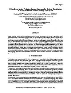
The Barcelona DWSN is currently operated by AGBAR1 . This network supplies drinking water to the Metropolitan Area of Barcelona (Catalonia, Spain). The considered part corresponds to the water supply network in charge of extracting water from the sources (rivers), transporting it towards the storage tanks, for final delivering it to users through the water distribution network. The aggregate network model considered in this paper is a simplification of the entire system, where groups of elements have been merged (Figure 1). In particular, the case study has 17 tanks (i.e., n = 17), 61 pumps and valves (i.e., m1 = 61), 25 demand sectors (i.e., q = 25), 11 nodes (splitting and merging water) and 9 water sources (rivers, aquifers and wells). See Ocampo-Martinez et al. (2013) for further details. The main control objective to be achieved in the Barcelona DWSN is to guarantee the satisfaction of consumer demands while minimizing the economic cost of water production and transport. This fact is achieved by including in the objective function of the MPC controller the following performance criteria2 for all discrete-time instants k ∈ Z+ : > `E (xk , uk ; cu,k , cx,k ) := c> u,k We uk ∆t + cx,k Wh xk , ( (xk − sk )> Ws (xk − sk ) if xk ≤ sk `S (xk ; sk ) := 0 otherwise,

`∆ (∆uk ) := ∆u> k W∆u ∆uk .

(19a) (19b) (19c)

The first goal, `E (xk , uk ; cu,k , cx,k ) ∈ R≥0 , corresponds to the economic cost of operation at time instant k, which has two parts cu,k := (c1 + c2,k ) ∈ Rm + . Those parts include both water production and electricity costs associated to water pumping. The former is included in c1 ∈ Rm + , while the latter is included in m c2,k ∈ R+ . Electrical cost varies during the day according to the tariff (usually with a daily periodicity). On the other hand, the cost cx,k ∈ Rn+ is associated to 1

Aguas de Barcelona, S.A. is the company in charge of the management of the drinking water network in Barcelona (Spain). 2 These performance criteria are quite general in the management of DWSN although from network to network some variations might be needed.

16

Figure 1: Barcelona DWSN aggregate diagram keep the water in the storage tanks. All prices are expressed in economic units per cubic meter (e.u./m3 ). The second goal, `S (xk ; sk ) ∈ R≥0 for all k, aims at maintaining the water tank volume up to a pre-established safety threshold sk ∈ Rn , expressed in m3 . This objective can be defined as `S (ξk ; xk , sk ) := ξk> Ws ξk , plus two additional convex constraints, i.e., xk ≥ sk − ξk and ξk ∈ Rn+ , for all k. The last goal, `∆ (∆uk ) ∈ R≥0 , penalizes the control signal variations ∆uk := uk − uk−1 ∈ Rm to guarantee a smooth operation of actuators, preserving their life as much as possible. The prioritization of these goals is established by means of a set of n n m weights We ∈ Sm ++ , Wx ∈ S++ , Ws ∈ S++ and W∆u ∈ S++ in their corresponding cost function. The inclusion of these goals into the MPC controller leads to state a multiobjective stage cost function for all k ∈ Z+ `(k, xk , uk , ξk ) := γ1 `E (xk , uk ; cu,k , cx,k ) + γ2 `∆ (∆uk ) + γ3 `S (ξk ; xk , sk ),

(20)

where γ1 , γ2 , γ3 ∈ R+ are weighting factors that allow to prioritize the impact of each goal over the network performance. Weight tuning is out of the scope of this paper, but the reader is referred to Barreiro-Gomez, Ocampo-Martinez, & Quijano (2015); Toro, Ocampo-Martinez, Logist, Van Impe, & Puig (2011) for systematic MPC tuning procedures. 17

4

3.8674

x 10

3.8673

V N ( k , x k , u pk )

3.8672

3.8671

3.867

3.8669

3.8668

3.8667

0

1

2

3

4

5

6

7

8

p m ax

9

10

11

12

13

14

15

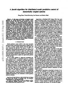
Figure 2: Open-loop cost decreasing of VN as function of the number of GaussJacobi iterations The MPC controller exploits the daily periodicity induced in the network dynamics by the daily periodic behaviour of the water demand and electricity prices. This is done by considering a prediction horizon N = 24 with a sampling time of one hour. This MPC controller represents the supervisory control layer of the water network, providing optimal flow set-points at the regulatory layer (PID and PLCs controlling the respectively valves and pump stations, which operate with a smaller sampling time).

4.2

Results Discussion

Figure 2 illustrates the convergence of Algorithm 1 at k = 0 using N = 24 hours. Note that open-loop cost is decreasing, showing a convergent behaviour as the number of iterations increases. Concerning the closed-loop performance, evaluated for a simulation horizon of 96 hours, Figure 3 presents some selected tank and pump behaviours achieved with the application of the proposed control approach summarized in Algorithm 1 for p = {1, 5, 10} and the corresponding evolution of the same elements when using the centralized standard MPC with terminal equality constraint reported in Grosso, Ocampo-Martinez, Puig, Limon, & Pereira. (2014) and the hierarchicallike decentralized MPC proposed in Ocampo-Martinez et al. (2011). These controllers are named CDMPC, CMPC and DMPC, respectively. From Figure 3, it can be seen that the approach proposed in this paper, i.e., CDMPC, achieves quite close behaviours to those obtained with the CMPC and clearly outperform18

7

#10

Tank 7

4

#10

1.8

Tank 10

4

1.6

6

#10

10

Tank 12

4

CMPC DMPC CDMPCp=1 CDMPCp=5

9

CDMPCp=10

1.4

volume [m3 ]

5

8 1.2

4

7 1

3

6 0.8

2

1

5

0.6

0

20

40

60

80

100

0.4

0

20

time [hours]

40

60

80

100

4

0

20

time [hours]

40

60

80

100

time [hours]

(a) Behaviour of water volumes in tanks Actuator 24

3

Actuator 29

0.3

Actuator 59

0.2

flow [m3 /hour]

0.18 2.5

0.25

2

0.2

1.5

0.15

0.16 0.14 0.12 0.1 0.08

1

0.1

0.5

CMPC DMPC CDMPCp=1 CDMPCp=5

0.06 0.04

0.05

0.02 0

0

20

40

60

time [hours]

80

100

0

0

20

40

60

80

100

0

CDMPCp=10

0

time [hours]

20

40

60

80

100

time [hours]

(b) Behaviour of water flows through actuators

Figure 3: Comparisons of behaviours from selected tanks and pumps ing the DMPC approach. Likewise, Table 1 presents the quantitative comparison among CDMPC (using p = {1, 5, 10}), CMPC, DMPC and, for completeness of the performed assessment, the multi-layer decentralized MPC (ML-DMPC) reported in OcampoMartinez et al. (2014) is also included into the comparisons. In this case, the closed-loop performance is compared in terms of both computational and economic costs. For each MPC approach, the average computational time (in s) needed to solve the optimization problems, as well as water, electricity and total costs (in e.u.) are presented. From these results, DMPC performs better that all other approaches in terms of average computational time but leading to a higher sub-optimality (compared to CMPC as a baseline) due to the loss of economic information inherent to the decentralization process. On the other hand, ML-DMPC presents better results than DMPC due to the use of an upper coor-

19

Table 1: Performance comparisons Controller approach CMPC DMPC ML-DMPC CDMPCp=1 CDMPCp=5 CDMPCp=10

Water Cost

Electricity Cost

Total Cost

CPU Time

96.468 171.136 110.720 106.455 106.443 106.444

86.317 63.940 86.659 82.900 82.907 82.905

182.785 235.076 197.379 189.355 189.350 189.349

17.493 5.787 5.819 19.910 100.588 201.218

dination layer, which updates (in a non-iterative manner) the cost of the shared control variables such that each local controller has an approximated global economic information. Finally, for the case of CDMPC, the overall closed-loop performance improves increasing the intermediate Gauss-Jacobi iterates but without converging to the MPC results. In particular, for the considered case study, the improvement rate is slow. The overall cost of CDMPC does not decrease considerably using p = 5 or p = 10, but without increasing the computational time remarkably. Thus, there exists a trade-off between the level of sub-optimality and the number of p-iterations. CDMPC presents a better performance than ML-DMPC considering the economic cost due to the use of a centralized model at each local CDMPC controller (no coordination layer is required). Moreover, ML-DMPC is non-iterative and its recursive feasibility is guaranteed by using adequate robustness constraints at the expense of reducing the economic performance. However, the average computational time related to ML-DMPC is considerably reduced compared to the CDMPC strategy. Thus, ML-DMPC is an appealing solution for large-scale networks because of its low complexity, its level of sub-optimality, and its computational time.

5

Conclusions

This paper presents an iterative distributed MPC formulation for its application to periodically time-varying generalized flow-based networks including convex constraints and strictly-convex economic cost functions. The distributed algorithm relies on the cooperation of local controllers. Such controllers use the centralized model and objective function of the system but optimizing only their corresponding control inputs. The communication strategy between subsystems is performed all-to-all. Thus, a reliable communication network is required. This approach has as main advantage the possibility of easily coping with the interactions related to both dynamic and static nodes of the network, without getting 20

complex the feasibility analysis. Different from other approaches reported in the literature, recursive feasibility of the cooperative algorithm does not rely on robustness constraints. Alternatively, it is based on convex combinations of the local solutions, which follow the suboptimal MPC philosophy, allowing the early termination of the distributed optimization before convergence. The scheme uses a periodically time-varying terminal penalty/region that forces the state to be within the optimal nominal periodic orbit at the end of the prediction horizon. This mechanism allows obtaining a priori bounds of the average performance of the closed-loop system. Specifically, the system performs better in average than the best periodic orbit. Moreover, the stability of the optimal periodic orbit can be guaranteed and, in case that the algorithm converges, a Nash equilibrium is achieved. As future work, the analytical reduction in the number of intermediate iterations should be developed since the rate of convergence towards the Nash equilibrium could be slow in some cases, implying higher computational times. Additionally, the extension of the proposed approach for being applied to non-linear systems and the deep study of systems with delays and robust control schemes (see, e.g., Bououden, Chadli, & Karimi (2016); Yao, Karimi, Sun, & Lu (2014)) will be also considered.

Acknowledgment This work has been partially funded by the Spanish Ministry of Science and Technology through the projects DEOCS (Ref. DPI2016-76493-C3-3-R) and HARCRICS (Ref. DPI2014-58104-R).

References Amrit, R., Rawlings, J., & Angeli, D. (2011). Economic optimization using model predictive control with a terminal cost. Annual Reviews in Control , 35 (2), 178-186. Angeli, D., Amrit, R., & Rawlings, J. (2012). On average performance and stability of economic model predictive control. IEEE Transactions on Automatic Control , 57 (7), 1615-1626. doi: 10.1109/TAC.2011.2179349 Barreiro-Gomez, J., Ocampo-Martinez, C., & Quijano, N. (2015). Evolutionary-game-based dynamical tuning for multi-objective model predictive control. In S. Olaru, A. Grancharova, & F. Lobo-Pereira (Eds.), Developments in model-based optimization and control (Vol. 464, p. 115-138). Springer Verlag. Blanchini, F., Rinaldi, F., & Ukovich, W. (1997). Least inventory control of multistorage systems with non-stochastic unknown inputs. IEEE Transactions on Robotics and Automation, 13 (5), 633-645.

21

Bououden, S., Chadli, M., & Karimi, H. (2016). A robust predictive control design for nonlinear active suspension systems. Asian Journal of Control , 18 (1), 122–132. doi: 10.1002/asjc.1180 Christofides, P., Scattolini, R., de la Peña, D. M., & Liu, J. (2013). Distributed model predictive control: A tutorial review and future research directions. Computers & Chemical Engineering, 51 , 21-41. Conejo, A., Castillo, E., Minguez, R., & Garcia-Bertrand, R. (Eds.). (2006). Decomposition techniques in mathematical programming. Berlin: Springer. Grosso, J., Ocampo-Martinez, C., Puig, V., Limon, D., & Pereira., M. (2014, June). Economic MPC for the management of drinking water networks. In Proc. european control conference (ecc) (p. 790-795). Strasbourg, France. Jilg, M., & Stursberg, O. (2013, July). Optimized distributed control and topology design for hierarchically interconnected systems. In Proc. european control conference (ecc) (p. 43404346). Kamelian, S., & Salahshoor, K. (2015). A novel graph-based partitioning algorithm for largescale dynamical systems. International Journal of Systems Science, 46 (2), 227-245. Kellett, C. (2014). A compendium of comparison function results. Mathematics of Control, Signals, and Systems, 26 (3), 339-374. Lee, J., & Angeli, D. (2014). Cooperative economic model predictive control for linear systems with convex objectives. European Journal of Control , 20 (3), 141-151. Lunze, J. (1992). Feedback control of large-scale systems. Great Britain: Prentice Hall. Motee, N., & Sayyar-Rodsari, B. (2003, June). Optimal partitioning in distributed model predictive control. In Proceedings of the American Control Conference (Vol. 6, p. 53005305). Negenborn, R., & Maestre, J. (2014, Aug). Distributed model predictive control: An overview and roadmap of future research opportunities. IEEE Control Systems Magazine, 34 (4), 87-97. Ocampo-Martinez, C., Bovo, S., & Puig, V. (2011). Partitioning approach oriented to the decentralised predictive control of large-scale systems. Journal of Process Control , 21 (5), 775-786. (Special Issue on Hierarchical and Distributed Model Predictive Control) Ocampo-Martinez, C., Puig, V., Cembrano, G., & Quevedo, J. (2013). Application of predictive control strategies to the management of complex networks in the urban water cycle. IEEE Control Systems, 33 (1), 15-41. Ocampo-Martinez, C., Puig, V., Grosso, J., & Montes-de-Oca, S. (2014). Multi-layer decentralized MPC of large-scale networked systems. In Distributed model predictive control made easy (p. 495-515). Springer. Rawlings, J., & Mayne, D. (2011). Postface to Model Predictive Control: Theory and Design. (http://jbrwww.che.wisc.edu/home/jbraw/mpc/postface.pdf)

22

Rawlings, J. B., & Stewart, B. T. (2008, October). Coordinating multiple optimization-based controllers: New opportunities and challanges. Journal of Process Control , 18 (9), 839-845. Riverso, S., Farina, M., & Ferrari-Trecate, G. (2013). Plug-and-play decentralized model predictive control for linear systems. IEEE Transactions on Automatic Control , 58 (10), 2608-2614. Šiljak, D. (1991). Decentralized control of complex systems. Academic Press. Stewart, B., Venkat, A., Rawlings, J., Wright, S., & Pannocchia, G. (2010). Cooperative distributed model predictive control. Systems & Control Letters, 59 (8), 460-469. Toro, R., Ocampo-Martinez, C., Logist, F., Van Impe, J., & Puig, V. (2011, August). Tuning of predictive controllers for drinking water networked systems. In Proceedings of the 18th IFAC World Congress (p. 14507-14512). Milano, Italy. Yao, D., Karimi, H., Sun, Y., & Lu, Q. (2014). Robust model predictive control of networked control systems under input constraints and packet dropouts. Abstract and Applied Analysis, V2014 (478567), 1-11.

A

Auxiliary developments for the proof of Theorem 1

In order to analyse the asymptotic stability of the closed-loop system, the following periodically time-varying rotated stage and terminal costs are considered: L(k, x, u) := `(k, x, u) − `(k, x¯?k , u¯?k ) + λ(k, x) − λ(k + 1, f (k, x, u)), V¯f (k, x) := Vf (k, x) − Vf (k, x¯?k ) + λ(k, x) − λ(k, x¯?k ).

(21) (22)

Theorem A.1 Consider the economic MPC formulation of problem (9) with a given period T ∈ Z≥1 . If Assumptions 3 to 7 hold, the asymptotic average performance of the closed-loop system xk+1 = f (k, xk , κN (k, xk ))

(23)

is better than the performance of the optimal periodic trajectories derived from (7), i.e., PT −1 PM `(k, x¯?k , u¯?k ) k=0 `(k, xk , uk ) ≤ k=0 . (24) lim sup M +1 T M →+∞ Proof. This result follows from the combination of preliminary results on MPC with periodic terminal equality constraint (Angeli et al., 2012) and MPC with fixed terminal region constraint (Amrit, Rawlings, & Angeli, 2011). Assume that PN (k, xk , dT , pT ) has a feasible solution for the current state xk ∈ XN (k), 23

which gives optimal input and state sequences denoted respectively as u?k = {u?k+t|k }i∈Z[0,N −1] and x?k = {x?k+t|k }i∈Z[0,N ] . Choose a candidate input sequence and its associated state sequence admissible in FN (k + 1) for the next time step, as follows: ˜ k+1 = {u?k+1|k , . . . , u?k+N −1|k , κf (k + N, x?k+N |k )}, u ˜ k+1 = {x?k+1|k , . . . , x?k+N |k , x?k+N +1|k }, x where x?k+N +1|k = f (k + N, x?k+N |k , κf (k + N, x?k+N |k )). Due to the terminal constraint (9d) and the periodic invariance property stated in Assumption 7, it holds x?k+N +1|k ∈ Xf (k + N + 1, x¯?k+N ). Moreover, the cost (9a) evaluated along these feasible candidate state/input sequences is given by ˜ k+1 ) = VN (k + 1, x?k+1|k , u

N −1 X

`(k + t, x?k+t|k , u?k+t|k ) + `(k + N, x?k+N |k , κf (k + N, x?k+N |k ))

i=1

+ Vf (k + N + 1, x?k+N +1|k ) = VN0 (k, xk ) − `(k, xk , u?k|k ) + `(k + N, x?k+N |k , κf (k + N, x?k+N |k )) − Vf (k + N, x?k+N |k ) + Vf (k + N + 1, x?k+N +1|k ).

From (11a) in Assumption 7, it follows that ˜ k+1 ) ≤ VN0 (k, xk ) + `(k, x¯?k , u¯?k ) − `(k, xk , u?k|k ). VN (k + 1, x?k+1|k , u ˜ k+1 ). Therefore, for all states By optimality, VN0 (k + 1, xk+1 ) ≤ VN (k + 1, x?k+1|k , u xk ∈ XN (k), it holds that VN0 (k + 1, xk+1 ) − VN0 (k, xk ) ≤ `(k, x¯?k , u¯?k ) − `(k, xk , u?k|k ). Taking averages on both sides of (25) gives PM V 0 (k + 1, xk+1 ) − VN0 (k, xk ) 0 = lim inf k=0 N M →+∞ M +1 PM `(k, x¯?k , u¯?k ) − `(k, xk , uk ) ≤ lim inf k=0 M →+∞ M +1 PT −1 PM ? ¯k , u¯?k ) `(k, xk , uk ) k=0 `(k, x = − lim sup k=0 . T M +1 M →+∞

(25)

(26a) (26b) (26c)

The left-hand side equality of (26) comes from Assumptions 3, 4 and 6, which imply that VN0 (k + 1, xk+1 ) − VN0 (k, xk ) is bounded. The right-hand side equality of (26) comes from the fact that the pair (¯ x?k , u¯?k ) is T -periodic for all k, then, the infinite horizon average cost is equal to the average cost of a single period (see (Angeli et al., 2012, Theorem 4)). Rearranging, one obtains the desired inequality (24), which completes the proof.  24

Lemma A.1 (Stability condition of the modified costs) Let Assumption 7 hold. The modified costs L and V¯f satisfy the following property for all k ∈ Z+ and all x ∈ Xf (k, x¯?k ): V¯f (k + 1, f (k, x, κf (k, x))) ≤ V¯f (k, x) − L(k, x, κf (k, x)). (27) Proof. Similarly to the proof of (Amrit et al., 2011, Lemma 9), the desired inequality comes from adding to both sides of (22) the term λ(k, x) + λ(k + 1, f (k, x, κf (k, x))), rearranging and considering Vf (k, xˆ?k ) = 0 and λ(k, xˆ?k ) = 0 for all k ∈ Z+ .  Lemma A.2 (MPC cost is less than terminal cost) Let Assumptions 3 to 7 hold, and denote by V¯N0 (k, xk ) the optimal solution to (9a) subject to (9b) and (9e) at time step k ∈ Z+ . Then, V¯ 0 (k, xk ) ≤ V¯f (k, xk ), ∀xk ∈ Xf (k, x¯? ), ∀k ∈ Z+ . (28) N

k

Proof. From Assumption 7, there exists a control law κf (k, xk ) ∈ Uk such that f (k, xk , κf (k, xk )) ∈ Xf (k + 1, x¯?k+1 ) for all xk ∈ Xf (k, x¯?k ) and all k ∈ Z+ . Due to the periodic positive invariance of the sequence of terminal regions, every κf (t, xt )) for time steps t > k is a suboptimal but feasible control action that keeps the state within the feasible set. Therefore, for all k ∈ Z+ and all xk ∈ Xf (k, x¯?k ) it follows by optimality that V¯N0 (k, xk ) ≤

N −1 X

L(k + t, xk+t , κf (k + t, xk+t )) + V¯f (k + N, xk+N )

i=0

= V¯f (k, xk ) +

N −1 X

(29)

(L(k + t, xk+t , κf (k + t, xk+t ))

i=0

+ V¯f (k + t + 1, xk+t+1 ) − V¯f (k + t, xk+t )). Then, applying (27) consecutively to the terms in the last summation of (29) leads to (28) and the claim is proved.  Lemma A.3 (Bounds on positive definite functions (Kellett, 2014)) Let ρ(x) : A → R≥0 be a positive definite function defined on a compact set A, i.e., zero at zero and strictly positive on x 6= 0. Then, there exist functions α1 , α2 ∈ K, such that α1 (x) ≤ ρ(x) ≤ α2 (x), ∀x ∈ A, k ∈ Z+ . (30) Lemma A.4 (Bounds on modified stage and terminal costs) Let Assumptions 3 to 7 hold, and let α1 and α ˜ 2 be K∞ functions. The rotated stage cost L and terminal cost V¯f satisfy, for all k ∈ Z+ , the following inequalities: L(k, xk , uk ) ≥ α1 (kxk − x¯?k k), ∀xk ∈ XN (k), ∀uk ∈ Uk , α1 (kxk − x¯?k k) ≤ V¯f (k, xk ) ≤ α ˜ 2 (kxk − x¯?k k), ∀xk ∈ Xf (k, x¯?k ). 25

(31) (32)

Proof 2 From (10), (21) and Assumption 5, it holds that L(k, xk , uk ) ≥ ρ(kxk − x¯?k k) for all (xk , uk ) ∈ Yk , which in addition to Lemma A.3, leads to (31). Consider now a trajectory starting in the terminal region, that is, xk ∈ Xf (k, x¯?k ), and driven by the terminal controller kf . Following the line of arguments in (Amrit et al., (31) that P2011, Lemma 11 and 12), it can be shown from (27) and ¯ V¯f (k, xk ) ≥ +∞ L(k, x , κ (k, x )). Hence, from (31) it follows that V (k, xk ) ≥ k f k f k=0 ? ¯ α1 (kxk − x¯k k) ≥ 0 for all k ∈ Z+ . In addition, from Assumption 6, Vf (k, xk ) is locally bounded and by definition V¯f (k, x¯?k ) = 0, thus, it can be upperbounded by a class K∞ function, i.e., V¯f (k, xk ) ≤ α ˜ 2 (kxk − x¯?k k) for all xk ∈ Xf (k, x¯?k ) and all k ∈ Z≥0 .

26