Mustafizur Rahman, Srikumar Venugopal and Rajkumar Buyya. Grid Computing and Distributed Systems (GRIDS) Laboratory. Department of Computer Science ...
A Dynamic Critical Path Algorithm for Scheduling Scientific Workflow Applications on Global Grids Mustafizur Rahman, Srikumar Venugopal and Rajkumar Buyya Grid Computing and Distributed Systems (GRIDS) Laboratory Department of Computer Science and Software Engineering The University of Melbourne, Australia {mmrahman, srikumar, raj}@csse.unimelb.edu.au
Abstract Effective scheduling is a key concern for the execution of performance driven Grid applications. In this paper, we propose a Dynamic Critical Path (DCP) based workflow scheduling algorithm that determines efficient mapping of tasks by calculating the critical path in the workflow task graph at every step. It assigns priority to a task in the critical path which is estimated to complete earlier. Using simulation, we have compared the performance of our proposed approach with other existing heuristic and meta-heuristic based scheduling strategies for different type and size of workflows. Our results demonstrate that DCP based approach can generate better schedule for most of the type of workflows irrespective of their size particularly when resource availability changes frequently.
1. Introduction Many of the large-scale scientific applications executed on present-day Grids are expressed as complex e-Science workflows [1][2]. A workflow is a set of ordered tasks that are linked by data dependencies [3]. A Workflow Management System (WMS) [3] is generally employed to define, manage and execute these workflow applications on Grid resources. A WMS may use a specific scheduling strategy for mapping the tasks in a workflow to suitable Grid resources in order to satisfy user requirements. Numerous workflow scheduling strategies have been proposed in literature for different objective functions [4]. However, the majority of these are static scheduling algorithms that produce a good schedule given the current state of Grid resources and do not take into account changes in resource availability. Critical path heuristics [5] have been used extensively for scheduling interdependent tasks in multi-
processor systems. These aim to determine the longest of all execution paths from the beginning to the end (or the critical path) in a task graph, and schedule them earliest so as to minimize the execution time for the entire graph. Kwok and Ahmad [6] introduced the Dynamic Critical Path (DCP) algorithm in which the critical path is dynamically determined after each task is scheduled. However, this algorithm is designed for mapping tasks on to homogeneous processors, and is static, in the sense that the schedule is only computed once for a task graph. In this paper, we extend the DCP algorithm to map and schedule tasks in a workflow on to heterogeneous resources in a dynamic Grid environment. We have extensively compared the performance of our algorithm, called DCP-G (Dynamic Critical Path for Grids), against well-known Grid workflow algorithms. The rest of the paper is organized as follows. In the next section, we describe existing heuristics and metaheuristics based workflow scheduling techniques on distributed systems such as Grid. The proposed DCP-G workflow scheduling algorithm is presented in Section 3. Experiment details and simulation results are presented in Section 4. Finally, we conclude the paper with the direction for future work in Section 5.
2. Related Work Generally, a workflow application is represented as a Directed Acyclic Graph (DAG) in which graph nodes represent tasks and graph edges represent data dependencies among the tasks with weights on the nodes representing computation and weights on the edges representing communication volume. Therefore, workflow scheduling problem is usually considered as a special case of the DAG scheduling problem. As the DAG scheduling problem is NP-complete, we rely on heuristics and meta-heuristics based scheduling strate-
gies to achieve the most efficient possible solution. In the following, we present some of the well-known heuristics and meta-heuristics for workflow scheduling on Grid systems. Myopic [7]: schedules an unmapped ready task, in arbitrary order, to a resource which is expected to complete that task earliest, until all tasks have been scheduled. It is considered as the simplest method for scheduling workflow applications. Min-Min [8]: is a list scheduling heuristic that assigns priority to the task based on its Expected Completion Time (ECT) on a resource. In every step of iteration, it discovers the task that has Minimum Expected Completion Time (MCT) among all the available tasks and assigns it to the resource that provides the MCT. This is repeated until all tasks are assigned. The intuition behind Min-Min is to consider all unmapped independent tasks during each mapping decision, whereas Myopic only considers one task at a time. Max-Min [8]: is similar to Min-Min except that in each iterative step, a task having the maximum ECT is chosen to be scheduled on the resource which is expected to complete the task at the earliest time. Intuitively, Max-Min attempts to minimize the total workflow execution time by assigning longer tasks to comparatively better resources. Both Min-Min and Max-Min have been used for scheduling workflow tasks in Pegasus [9]. Heterogeneous Earliest Finish Time (HEFT) [10]: used in the ASKALON workflow manager [7][11], is a well-established list scheduling algorithm which assigns higher priority to the workflow task having higher rank value. It calculates rank value based on the average execution time for each task and average communication time between resources of two successive tasks, where the tasks in the ‘critical path’ get comparatively higher rank values. In the resource selection phase, tasks are scheduled in the order of their priorities and each task is assigned to the resource that can complete the task at the earliest time. The advantage of using this technique over Min-Min or Max-Min is that while assigning priorities to the tasks it considers the entire workflow rather than focusing on only unmapped independent tasks at each step. Greedy Randomized Adaptive Search Procedure (GRASP) [12]: is an iterative randomized search technique. In GRASP, a number of iterations are conducted to search a possible optimal solution for mapping tasks on resources. A solution is generated at each iterative step and the best solution is kept as the final schedule. This searching procedure terminates when the specified termination criterion, such as the
completion of a certain number of iterations, is satisfied. GRASP can generate better schedules than the other scheduling techniques stated previously as it searches the whole solution space considering entire workflow and available resources. Genetic Algorithm [13]: is also meta-heuristic based scheduling technique such as GRASP. It allows a high quality solution to be derived from a large search space in polynomial time by applying the principles of evolution. Instead of creating a new solution by randomized search as in GRASP, GA generates new solutions at each step by randomly modifying the good solutions generated in previous steps which results a better schedule within less time.
3. The Proposed DCP-G Algorithm For a task graph, the lower and upper bounds of starting time for a task are denoted as the Absolute Earliest Start Time (AEST) and the Absolute Latest Start Time (ALST) respectively. In the DCP algorithm [6], the tasks on the critical path have equal AEST and ALST values as delaying these tasks affects the overall execution time for the task graph. The first task on the critical path is mapped to the processor identified for it. This process is repeated until all the tasks in the graph are mapped. However, this algorithm is designed for scheduling all the tasks in a task graph with arbitrary computation and communication times to a multiprocessor system with unlimited number of fully connected identical processors. But, Grids [14] are heterogeneous and dynamic environments consisting of computing, storage and network resources with different capabilities and availability. Therefore, to work on Grids, the DCP algorithm needs to be extended in the following manner: • For a task, the initial AEST and ALST values are calculated for the resource which provides the minimum execution time for the task. The overall objective is to reduce the length of the critical path at every pass. We follow the intuition of the Min-Min heuristic in which a task is assigned to the resource that executes it fastest. • For mapping a task on the critical path, all available resources are considered by DCP-G, as opposed to the DCP algorithm, which considers only the resources (processors) occupied by the parent and child tasks. This is because, in the latter case, the execution time is not varied for different processors, and only the communication time between the tasks could be reduced by assigning tasks to the same resource. However, in Grids, the communication and computation times are both liable to change because of resource heterogeneity.
•
When a task is mapped to a resource, its execution time and data transfer time from the parent node are updated accordingly. This changes the AEST and ALST of succeeding tasks.
3.1. Calculation of AEST and ALST in DCP-G In DCP-G, the start time of a task is not finalized until it is mapped to a resource. Here, we also introduce two more attributes: the Absolute Execution Time (AET) of a task which is the minimum execution time of the task, and Absolute Data Transfer Time (ADTT) which is the minimum time required to transfer the output of the task given its current placement. Initially, AET and ADTT are calculated as, AET(t) =
Task_size(t) max k ∈Re sourceList {PC(Rk )}
ADTT(t) =
Task_output_size(t) max k ∈Re sourceList {BW(Rk )}
Where, PC ( Rk ) and BW ( Rk ) are processing capability and transfer capacity i.e. Bandwidth of resource Rk respectively. Whenever a task t is scheduled to a resource, the values of AET (t ) and ADTT (t ) are updated accordingly. Therefore, the AEST of a task t on resource R, denoted by AEST (t , R) , is recursively defined as, AEST(t,R) = max {AEST(t k ,Rt k ) + AET(t k ) + Ct,t k (Rt ,Rt k )} 1≤ k ≤ p
where, t has p parent tasks, tk is the kth parent task and, AEST (t , R ) = 0 ; if t is an entry task. Ct,tk (Rt , Rtk ) = 0 ; if Rt = Rtk Ct ,tk ( Rt , Rtk ) = ADTT (t k ) ; if t and tk are not scheduled.
Here, the communication time between two tasks is considered to be zero if they are mapped to the same resource, and equal to the ADTT of parent task, if the child is not mapped yet. Using this definition, the AEST values can be computed by traversing the task graph in a breadth-first manner beginning from the entry tasks. Once AESTs of all the tasks are computed, it is possible to calculate Dynamic Critical Path Length (DCPL) which is the schedule length of the partially mapped workflow. DCPL can be defined as, DCPL = max{ AEST (t i , Rti ) + AET (t i )} 1≤i ≤ n
where, n is the total number of tasks in the workflow. After computing the DCPL, the values of ALST can be calculated by traversing the task graph in a breadth-first manner but in the reverse direction. Thus, the ALST of a task t in resource R, denoted as ALST (t , R ) , can be recursively defined as,
ALST(t,R) = min {ALST(tk ,Rt k ) − AET(t) − Ct,t k (Rt ,Rt k )} 1≤ k ≤ c
where, t has c child tasks, tk is the kth child task and, ALST (t , R ) = DCPL − AET (t ) ; if t is an exit task. Ct ,tk ( Rt , Rtk ) = 0 ; if Rt = Rtk Ct ,tk ( Rt , Rtk ) = ADTT (tk ) ; if t and tk are not mapped.
As in DCP, a task in DCP-G is considered to be on the critical path if its AEST and ALST values are equal. In order to reduce the value of DCPL at every step, the task selected for scheduling is the one that is on the critical path and has no unmapped parent tasks.
3.2. Resource Selection After identifying a critical task, we need to select an appropriate resource for that task. We select the resource that provides the minimum execution time for that task. This is discovered by checking all the available resources for one that minimizes the potential start time of the critical child task on the same resource, where the critical child task is the one with the least difference of AEST and ALST among all the child tasks of the critical task. Finally, the critical task is mapped to the resource that provides earliest combined start time.
3.3. DCP-G Example Figure 1 illustrates the DCP-G algorithm with a step-by-step explanation of the mapping of tasks in a sample workflow. The sample workflow consists of five tasks denoted as T0, T1, T2, T3 and T4 with different execution and data transfer requirements. The length and size of the output of each task shown in Figure 1(a) are measured in Million Instructions (MI) and GigaBytes (GB) respectively. The tasks are to be mapped to two Grid resources R1 and R2 with processing capability (PC) and transfer capacity i.e. Bandwidth (BW) as indicated at the bottom of Figure 1. First, the AET and ADTT values for each task are calculated as shown in Figure 1(a). Then using these values, AEST and ALST of all the tasks are calculated according to Section 3.1 (Figure 1(b)). Since T0, T2, T3 and T4 have equal AEST and ALST, they are on critical path with T0 as the highest task. Hence, T0 is selected as the critical task and mapped to resource R1 which gives T0 the minimum combined start time. At the end of this step, the schedule length of the workflow, i.e. DCPL is 890. Similarly, in Figure 1(c), T2 is selected as critical task and mapped to R1. As both T0 and T1 are mapped to R1 and the data transfer time of T0 is now zero, the AEST and ALST of all the tasks are changed and the schedule length becomes 850 (Figure 1(d)). In the next step, T3 is mapped to R1 as well and
150000 MI 100 \ 40
T0
T0
R1 0/0
T0
R1
T0
0/0
0/0
1 GB 300000 MI 200 \ 80
R1
T1
T2
300000 MI 200 \ 80
140 / 560
T1
T2
140 / 560
140 / 140
T1
T2
140 / 520
140 / 140
T1
T2
100 / 100
2 GB 2 GB 600000 MI 400 \ 20
T3
T3
T3
420 / 420
T3
420 / 420
380 / 380
0.5 GB 75000 MI 50 \ 0
T4
840 / 840 Task size
T
T0
0/0
140 / 440
T2
T0
100 / 100
180 / 310
0/0
R1
T2
R1
T3
800 / 800
T0
(d)
180 / 310
100 / 100
T3
Task
R1
T2
R1
300 / 300
Final Schedule
0/0
R2
T1
T4
720 / 720
DCPL = 770 T2 R2
R1
T3
300 / 300
T4
700 / 700
R2
PC = 1200 MIPS BW = 200 Mbps
T
0
T1
R2
180
430
T2
R1
100
300
T3
R1
300
700
T4
R1
700
750
300 / 300
T4
(g) Scheduled Task
0
DCPL = 750
(f)
PC = 1500 MIPS BW = 100 Mbps
End
R1
R1
DCPL = 770 T4 R1
(e)
Resource Start
T0
100 / 100
R1 720 / 720
T4
DCPL = 850 T3 R1
(c) R1
R2
T1
T4
DCPL = 890 T2 R1
(b) R1
R1
T1
840 / 840
DCPL = 890 T0 R1
AET \ ADTT
(a) R1
T4
T
Critical Task
T
(h)
AEST / ALST
T
R: Task T is assigned to Resource R
Figure 1. Example of workflow scheduling using DCP-G algorithm the DCPL is reduced to 770 as the data transfer time for T2 is zero. Now T4 is the only task remaining on the critical path (Figure 1(e)). However, one of its parent tasks, T1, is not mapped yet and therefore T1 is selected as critical task. As T2 and T3 are already mapped to R1, the start time of T1 on R1 is 700. Therefore, T1 is mapped to R2 as its start and end times on R2 are 180 and 430 respectively. Finally, when T4 is mapped to R1 (Figure 1(g)), all the tasks have been mapped and the schedule length can not be improved any further and a schedule length of 750 is obtained. The final schedule generated by DCP-G is shown in a table in Figure 1(h).
4. Performance Evaluation We evaluate DCP-G by comparing the schedules produced by it against those produced by the other algorithms described previously for a variety of workflows in a simulated Grid environment. In this section, first we describe our simulation methodology and setup, and then present the results of experiments.
4.1. Simulation methodology We use GridSim [15] to simulate the application and Grid environment for our simulation. We model different entities in GridSim in the following manner. Workflow model. We implement a workflow generator that can generate various formats of weighted
pseudo-application workflows. The following input parameters are used to create a workflow. • N, the total number of tasks in the workflow. • α, the shape parameter represents the ratio of the total number of tasks to the width (i.e. maximum number of nodes in a level). So width W =
N α
• Type of workflow: Our workflow generator can generate three types of workflow namely parallel workflow, fork-join workflow and random workflow. Parallel workflow: In parallel workflow [16], a group of tasks creates a chain of tasks with one entry and one exit task and there can be several such chains in one workflow. Here, one task is dependent on only one task, but the tasks at the head of chains are dependant on entry task and the exit task is dependant on the tasks at the tail of chains. Number of levels in a parallel workflow can be specified as, Number of levels =
N −2 W
Fork-join workflow: In fork-join workflow [2], forks of tasks are created and then joined. So, there can be only one entry task and one exit task in this kind of workflow but the number of tasks in each level depends on total number of tasks and the width in that level, W. Number of levels in fork-join workflow can be specified as, Number of levels =
N W +1
Random workflow: In random workflow, dependency and number of parent tasks of a task which equals to the indegree of a node in DAG representation of the workflow, is generated randomly. Here, task dependency and the indegree are calculated as,
Maximum Indegree (Ti) = W 2
Minimum Indegree (Ti) = 1 Parent (Ti)= {Tx| Tx ∈ [T0….Ti-1]};if Ti is not a root task; where, x is a random number and 0