A Dynamic Medial Axis Model for Sensor Networks - TAMU Computer

A Dynamic Medial Axis Model for Sensor Networks Lan Lin and Hyunyoung Lee Department of Computer Science, University of Denver {llin,hlee}@cs.du.edu

Abstract An important property in a sensor network is the monitoring of temporal changes of hazardous situations such as forest fires. Rescue groups need to be aware of dynamic changes that affect their rescue efforts. In this paper, we discuss a sensor network model that provides a good abstraction of geometric and topological features of a dynamically changing sensing environment. This model enables efficient path planning and navigation using localized algorithms. We propose a dynamic medial axis model that represents shapes and changes of shapes in a geometric space. We develop distributed algorithms to capture the dynamic network topologies. Dynamic medial axis allows rescue teams to find a short path to safety in a changing environment. We show that our dynamic medial axis algorithms provide good approximations to the true medial axis and our routing scheme generates short and safe routes. The simulation results show that the routes found by our scheme are near-optimal.

1. Introduction Sensor network is a new bridge between the physical world and the virtual world of information. Until recently, sensor network research has been primarily focused on technologies for collecting information from the physical world, such as habitat monitoring [12] or structural monitoring [13]. Some more recent work [1, 6] started to view sensor networks as reactive systems, that is, sensors can not only detect hazards such as wildfires or chemical leaks, but also guide navigation of mobile agents in the presence of dangers or obstacles. This is the problem we discuss in this paper. One important characteristic of sensor networks that has not been sufficiently explored is the temporal property of the objects being monitored, for example, the continuous change of the boundary of an untrespassable obstacle such as chemical leaks of certain density. In this paper we propose a sensor network model for ap-

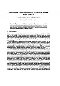
plications in motion planning and navigation guidance in changing environments using stationary sensors deployed in a two-dimensional space. The key idea of our design is based on the observation that sensor networks are good approximations of the geometric environment they are observing. Since only sensors that are in the vicinity of each other can directly communicate, the network topology is highly correlated to the geometric information that reflects the underlying structure of the physical environment. A good abstraction of the complex geometric shape and topological features is the foundation of our design. We use medial axis (a.k.a. skeleton) that has been studied in computational geometry for an efficient representation of shapes. Defined as the set of points with at least two closest neighbors on the boundaries of the shape, medial axis has been used in research areas such as robot motion planning [10] and surface reconstruction [3]. An example of medial axis for a sensor field, shown in Figure 1, is composed of the medial axis nodes, represented by the blue (thicker) dotted line, and paths from medial axis nodes to the boundary of the field, represented by the black (thinner) dotted lines. The medial axis is represented by a dynamic medial axis graph (DMAG); a dynamic graph of a size proportional to the number of geometric features. This DMAG is compact and is known to every medial axis sensor. Figure 1 shows the DMAG of two vertices, a and b, one edge, and one self-loop. To capture the dynamic change of obstacle regions, the medial axis of sensor networks are to be modified continuously as obstacles emerge or change shapes. We develop distributed algorithms for constructing and maintaining the dynamic medial axis in a sensor network. Our algorithms use only local knowledge to make adjustments to the medial axis but result in a near-optimal global solution. A good abstraction of the changing geometric and topological features, dynamic medial axis is a suitable roadmap for navigation in changing environments. The goal of our path planning scheme is to find an approximate shortest path that avoids changing obstacle regions. Our scheme supports localized routing with only the knowledge of the source and destination

b

A

a

e d

b

a

f

Figure 1. Left: An example of medial axis, medial axis nodes, and their routes to the boundary of a closed region. Right: The corresponding dynamic medial axis graph.

B

S

t

c C

Figure 2. An example of dynamic medial axis with three regions.

locations. It runs in two phases. First, an approximate as node e in Figure 2, with boundaries of A and C. The shortest safe path from source to destination is found uschords of e are the line segments connecting e to the ing DMAG, The navigation is taken place as each sensor boundaries of A and C. node guides the mobile agent on a safe and short path. We define a medial axis vertex as a medial axis point The maintenance of dynamic medial axis and the path with at least three closest points on the boundary (e.g., planning and execution are all performed in a localized node a, b, c, and d in Figure 2). A medial axis edge is manner, therefore our schemes are scalable. Experimena line segment on a medial axis with two medial axis tal results show that our scheme produces routing path vertices as endpoints, such as line segment ad, bd, and of length close to optimal path length. cd in Figure 2. A medial axis segment is composed of Our contributions. First, our dynamic medial axis those medial axis points and medial axis edges that are based model captures the continuous geometric and topothe closest to one obstacle. A medial axis region is the logical changes of a sensor field. Second, the construcarea enclosed by a medial axis segment. A medial axis tion and dynamic adjustment of the medial axis is lightweight. graph is the set of medial axis vertices and the medial Third, our medial axis based path planning algorithm is axis edges that connect them. A medial axis segment is efficient, localized, and scalable. a subgraph of medial axis graph. The rest of the paper is organized as follows. In Section 2, we discuss properties of dynamic medial axis in Lemma 2.1. No two chords intersect except at the mecontinuous Euclidean space. In Section 3, we present dial axis points. algorithms for the construction and maintenance of dyProof. See Lemma 3.2 in [5]. namic medial axis in sensor field and the routing scheme using dynamic medial axis. In Section 4, we present the In this paper we consider small continuous changes to simulation results. In the last two sections, we discuss continuous boundary curves in time. It was proved [7] related works and our conclusions. that for a bounded open set with smooth C 2 -boundary a small C 2 -perturbation of ∂M induces a small perturba2. Dynamic medial axis in continuous Eution of the medial axis of ∂M . Therefore a small conclidean space tinuous change to a continuous boundary curve results in a small change to the medial axis edge which remains continuous. 2.1 Dynamic medial axis A point p in M is identified with name ID(p) = (x(p), y(p), dx (p), dy (p)), where x(p) ∈ A, y(p) ∈ The definition of medial axis [4] for a continuous ∂M , dx (p) = |p, x(p)|, and dy (p) = |p, y(p)|, where curve in an Euclidean plane is as follows. The medial |p, q| denotes the Euclidean distance between points p axis of a curve F is a set of points in the plane, each of and q. Our naming scheme guarantees that each point in which has two or more closest points in F . Let M be M is assigned a unique name. a bounded open set in R2 , ∂M the boundary curve of M , and A the medial axis of ∂M . For each point a on 2.2 Routing infrastructure the medial axis, there exists a maximal disk inside of M with two or more tangent points on ∂M . We call a a medial axis point. A line segment that connects a meThe naming scheme provides a Cartesian coordinate dial axis point a with its tangent point on ∂M is called system for the points inside region M . The medial axis a chord of a. An example of medial axis point is shown A and the chords of medial axis vertices partition M

y y’b p p’ x x’ a

Figure 3. Illustration of proof of Theorem 2.2.

into a set of cells {Ci }, i = 1, . . . , m. Each cell C is bounded by two chords, a medial edge and a segment of the boundary ∂M . We define a k-avenue as the collection of points p in M with dx (p) = k. We define an l-street as a chord in M with medial axis point l. An m-contour is the collection of points p in M with dy (p) = m. By the definition of a chord, an l-street in M is a continuous line segment. Theorem 2.2. For a cell C bounded by two chords, c1 and c2 , a medial axis edge A, and a segment of the boundary ∂M , there exists a continuous curve between point p and point q, where p ∈ c1 and q ∈ c2 . Proof. Let the slope between dx (p) and dx (q) be k. We show that for any point p in C, there exists a point p′ on dx (p) + kε avenue within distance ε, for any |k|ε > 0. Figure 3 illustrates the proof. Suppose p is on a chord xy, where x ∈ A, y ∈ ∂M . Let dR (p, q) be the shortest distance between points p and q in domain R. Since both the medial axis A and the boundary ∂M are continuous, we can find a chord x′ y ′ , where x′ ∈ A, y ′ ∈ ∂M , such that dA (x, x′ ) ≤ δ, d∂M (y, y ′ ) ≤ δ, δ = ε/(1 + |k|). We first pick a chord ab with a ∈ A, b ∈ ∂M such that dA (x, a) ≤ δ. If d∂M (y, b) ≤ δ, we take ab as the chord x′ y ′ . Otherwise we take a point y ′ on ∂M where y ′ is between y and b and d∂M (y, y ′ ) ≤ δ. Let the chord y ′ is on be x′ y ′ . Then, x′ is between x and a on A and by Lemma 2.1, dA (x, x′ ) ≤ dA (x, a) ≤ δ. Choose the point p′ on the chord x′ y ′ where dx (p′ ) = dx (p) + kδ. Then |xp| − |k|δ ≤ |x′ p′ | ≤ |xp| + |k|δ, which gives |pp′ | ≤ |xp| − |x′ p′ | + dA (x, x′ ) ≤ (1 + |k|)δ = ε.

2.3

Routing scheme

Our routing scheme is to find a path for a point c in M moving from the source p to the destination q with no intersections with the boundary ∂M . Since ∂M changes in time, the routing scheme considers several dynamic factors: the moving speed of c, and the moving speed and direction of ∂M . Dynamic medial axis graph (DMAG). The change of the boundary in time results in a change of the medial

axis. To capture the dynamics of medial axis, we associate with each medial axis edge two weights, Wlen , the length of the line segment connecting the two end points of the edge, and Wtime , the available time, the time the edge is available before it is altered due to the topological change introduced by boundary variations. As a boundary segment moves, we calculate the Wtime of the corresponding medial axis edge by the moving speed of the boundary, Vbound , and the distance between the closest point on the boundary and the edge, Dbound . The available time of an edge is Wtime = Dbound /Vbound . The two weights are updated periodically and are stored at the two medial axis vertices. Thus the DMAG is a dynamic graph since the vertices, edges, and the weights of edges vary in time. 2.3.1 Medial axis and contour routing Given moving speed Vc of point c, routing from a source p to a destination q is performed using the medial axis A and contours. Let ID(p) = (x(p), y(p), dx (p), dy (p)) and ID(q) = (x(q), y(q), dx (q), dy (q)). First, we find the shortest path SPA (x(p), x(q)) on A, the path whose end point has the shortest Euclidean distance to x(q). This is because a safe passage to x(q) is not guaranteed due to the dynamicity of boundaries. Each medial axis edge ei is assigned a time cost, Ti , for c to travel through the edge, where Ti = Wlen,i /Vc . Using a shortest path algorithm, we can find the shortest path whose end point is closest to x(q). The algorithm is modified to add a check on the availability of an edge. An edge is available only if Wtime is not expired when c reaches the edge. The path found is only for medial axis edges. To reach the medial axis, the moving point c needs to route from p to x(p). The change of the boundary ∂M can be one of two kinds: either the boundary is moving toward the medial axis edge, or the boundary is moving away from the edge. In the first case, the boundary may reach the medial axis edge or cover part of the space inbetween the medial axis edge and the boundary. In the second case, both the medial axis edge and the space inbetween the edge and the boundary are unaffected. We propose routing scheme for both cases. Consider the cell C bounded by two chords, a medial axis edge, and a segment of the boundary ∂M . For the first case, the moving point c routes toward the medial axis vertex on the shortest continuous curve not intersecting the moving boundary. We further divide the second case into two cases. If the next medial axis vertex on the path makes a left turn, route toward the current medial axis vertex on the shortest continuous curve. If the next medial axis vertex makes a right turn, route on the shortest continuous curve toward the y(q)-contour. An example

is shown in Figure 2. As the boundaries of the three regions A, B and C change shape, indicated by the arrows, the medial axis changes accordingly. A route from source S to a destination is shown as the thick light dotted line (in green).

3. Dynamic medial axis in discrete sensor field In this section we apply to a discrete sensor field, the ideas of dynamic medial axis based naming and routing scheme discussed in the previous section. We consider the changes of obstacle shape and accordingly, the dynamic reconstruction of medial axis and the routing scheme for mobile agents in the sensor field.

3.1

Initial construction of medial axis

The initial construction of medial axis of the sensor field is as described in [5]. Nodes on the boundary of the field simultaneously broadcast messages that are subsequently propagated toward the interior of the field. A node is on the medial axis if it has equal hop counts to two closest boundary nodes. A medial axis segment is connected to the boundary by chords composed of nodes on the message path from the boundary. A node a is the downstream neighbor of another node b on a chord if the medial axis node sends message to the boundary through a to b. Node b is called the upstream neighbor of node a. The distance between two sensors is defined as the number of hops taken for message communication between them. The distance between neighboring sensors is one hop. We represent the medial axis using a weighted graph G = (V, E), where V is the set of medial axis vertices and E is the set of medial axis edges. Each edge in the graph is associated with two weights: the length Wlen and the available time Wtime . The length is defined as the number of hops between the two medial axis vertices. The available time is calculated by the moving speed of the boundary and the distance from the closest point on the boundary to the edge. The moving speed of the boundary is estimated by the sensors on the boundary of the obstacle. A copy of the graph is stored at each medial axis node. An obstacle in a sensor field is defined as a region that is untrespassable when certain conditions are met, for example, an obstacle caused by a chemical leak is a region where the sensor readings of the chemical density are above certain value. The boundary of an obstacle is composed of nodes that are inside an obstacle but have neighboring nodes whose readings are within the threshold. Each obstacle is assigned an identifier. The

identifier 0 is reserved for the boundary of a sensor field, i.e., we consider the region outside a sensor field as an obstacle. To avoid naming conflicts of emerging obstacles, the count of current obstacles is kept on on each medial axis node. To name an obstacle, one sensor on the boundary of the new obstacle is elected to request the medial axis node for an identifier bigger than the count. Assumptions We make the following assumptions in this paper. First, sensors are deployed uniformly on a physical surface. Second, boundary nodes initiate the medial axis construction at approximately the same time and messages travel at approximately the same speed. Third, every sensor has a unique ID. Fourth, sensors function correctly throughout their lifetimes. Faulty sensors and mechanisms for handling faulty sensors are beyond the concerns of this paper. Last, we assume an upper-bound on the spreading speed of a danger and that the speed of message communication is faster than the speed of any danger spreading.

3.2

Construction of dynamic medial axis

The continuous change of obstacle regions results in the dynamic adjustment of the medial axis. We consider five kinds of changes: the emergence of obstacle, two basic types of boundary change, expanding and shrinking, the disappearing of obstacle, the merging of two obstacles, and the dividing an obstacle into two. 3.2.1 New obstacle First, we consider the emergence of obstacles, such as, outbreaks of fire or leaks of harmful chemicals. Figure 4 shows an example: In (a), two obstacles are being monitored in the sensor field. The dotted lines represent the current medial axis. Suppose there emerges another obstacle, the location of which may be one of the three cases as shown in (b). Case 1 and 2 are equivalent if we view the region outside the field boundary as an obstacle. Case 3 can be treated as multiple obstacles of case 2 by dividing the obstacle region along the medial axis segments. Thus, we can design one algorithm to solve all three cases. Our algorithm is based on the observation that any location within a medial axis region is closer to the obstacle of the region than to any obstacles outside the region. Since the observation holds true for emerging regions, the new medial axis can be generated by sending out messages from the boundary of the new obstacle until the messages reach those nodes whose distances to an existing obstacle are equal to their distances to the new obstacle. Those nodes form the boundary of the new medial axis region containing the new obstacle.

000 111 111 000 000 111 000 111 000 111

1111 0000 0000 1111 0000 1111 0000 1111 0000 1111 0000 1111 0000 1111

1

000 111 111 000 000 111 000 111 000 111

2 3

0000000 1111111 0000000 1111111 1111111 0000000 0000000 1111111 0000000 1111111 0000000 1111111 0000000 1111111 0000000 1111111 000000 111111 000000 111111 000000 111111 000000 111111

111 000 000 111 000 111 000 111 000 111 000 111 000 111

B

a

(a)

1

A

b 2 3 4 c 5

(b)

Figure 4. Emergence of new obstacle.

For a sensor that is not inside an obstacle and not a neighbor of a boundary node of an obstacle, when its readings are above certain threshold for α times in the last ω time units [2], the sensor concludes that it is inside an obstacle region. It then sends messages to its neighbors requesting their decisions on a new obstacle. If the decisions are all positive, the sensor concludes that itself is inside the obstacle. If the decisions of some of its neighbors are negative, the sensor concludes that itself is on the boundary of the obstacle and uses local flooding to connect with other sensors on the boundary of the obstacle. Constructing a dynamic medial axis. Every sensor maintains two types of counters: dm , the distance from medial axis to the sensor, and do , the distance from an obstacle to the sensor, both of them are in terms of the number of hops. Messages are broadcast from the boundary of the obstacle. Each message carries a sender ID and a counter that records the distance the message has been propagated. The sensor on the boundary of the new obstacle broadcasts the message with the counter set to 1. Upon receiving the message for the first time, each sensor checks if the counter is equal to its own counter, do . If so, the sensor concludes that itself is on the new medial axis. If the counter is less than its own counter, it broadcasts the message with the counter incremented by 1. Otherwise, it drops the message. All the sensors on the new medial axis find its neighboring new medial axis nodes to form a medial axis segment. To join the new medial axis segment with the existing medial axis, the sensors on the intersections of the two send messages to its neighbors on the existing medial axis of the change. Theorem 3.1. The algorithm correctly constructs a dynamic medial axis. Figure 5 illustrates the proof of the theorem. The light dotted line indicates the existing medial axis with one obstacle A. The dark dotted line indicates the new medial axis with the new obstacle B. By the property of medial axis, we know that line 1 and line 2 are of the same length. The new medial axis edge ab that separates

Figure 5. Illustration of proof of Theorem 3.1.

A and B indicates that line 3 has the same length as line 1 by the property of medial axis. Therefore, line 3 is of the same length as line 2. The intersection points are where the message sending stops in the algorithm. The message sent along line 4 will stop at the intersection c with line 5, where the distance from c to the boundary of B is equal to that from c to the sensor field boundary, i.e., the lengths of line 4 and line 5 are equal. 3.2.2 Expanding and shrinking of obstacle A boundary node periodically inquires its upstream neighbor (a non-boundary node) of its readings. If the readings are above certain threshold for certain time periods, the boundary node concludes that an expansion of the boundary has occurred. If the boundary node’s own reading is below certain threshold for certain time periods, the node concludes that a shrinking of the boundary has occurred. In both cases, the medial axis is to be updated to reflect the change. The sensors on the boundary of the obstacle send message to the medial axis nodes around the obstacle. The message carries the boundary change in terms of the number of hops, m, from the previous boundary, where m < 0 for expanding and m > 0 for shrinking. Sensors on the message path add m to their counter do for that obstacle. Upon receiving the message, each medial axis node broadcasts a message to its neighbor on the other side of the medial axis. The message carries a counter set to be the node’s counter do for that obstacle. The messages stop at the sensors whose do for another obstacle equals the counter in the message. Those sensors become the new medial axis nodes. Note that the medial axis vertices of the existing medial axis segment around the obstacle are changed. The updated DMAG is propagated to all medial axis nodes. When two medial axis edges are within communication range of each other, they are merged into one edge. There can be only one case when the boundary is concave as shown in Figure 6(a). The medial axis nodes detect within their radio range some medial axis nodes other than their current neighbors. The nodes elect one edge to be the medial axis edge and make the two end nodes of the segment the new medial axis ver-

(a)

(b)

Figure 6. Adjustment of medial axis edges.

tices, shown in Figure 6(b). 3.2.3

Disappearing of an obstacle

When the number of boundary nodes of an obstacle is below certain threshold, the obstacle region is considered disappeared. To adjust the medial axis structure, the medial axis nodes initiate the construction of a medial axis segment by sending message to their downstream neighbors. The message contains the identifier of the other obstacle the node is closest to and a counter initially set to be the number of hops to that obstacle. The counter is incremented by one at each forwarding. The new medial axis segment is the set of nodes that are at equi-distance to two or more obstacles. 3.2.4

Merging two obstacles

The merging of two obstacles happens when the medial axis nodes detect that they are inside an obstacle region. A direct way of the detection is when their sensor readings are above certain threshold. An indirect way is when they are a few hops away from two obstacles. Our algorithm uses the second approach. Either way the medial axis nodes conclude that the medial axis edge they belong to is no longer traversable. The medial axis vertices at both ends of the edge update the DMAG. 3.2.5

Dividing an obstacle into two

When an obstacle region keeps changing its shape, it may divide into several disconnected regions. We only consider the case that one obstacle is divided into two. The division of an obstacle into multiple regions can be derived accordingly. When an obstacle region is changing into two regions, some nodes inside the region become boundary nodes. They initiate the local flooding of message to construct the medial axis segment between the new boundaries of the two regions.

3.3

Routing scheme

Given a source point p and a destination point q, dynamic medial axis based routing protocol runs as fol-

lows: 1. In the route planning phase, find the path SPA (x(p), x(q)) in the DMAG A; 2. Route toward the medial axis vertex of an edge on SPA (x(p), x(q)) if the corresponding boundary to the medial axis edge is approaching the edge; 3. Route in parallel to an edge of SPA (x(p), x(q)) if the corresponding boundary is receding from the edge and the next edge makes a left turn; 4. Route toward y(q) − contour if the corresponding boundary is receding and the next edge makes a right turn; 5. Route on y(q) − contour to reach the destination q. We first consider the route planning using the dynamic medial axis. To navigate from a location S in the sensor field to another location T , a mobile agent first communicates with a neighboring sensor requesting a route from S to T . The sensor sends the request to the medial axis node it connects to. The medial axis node calculates the shortest route on the medial axis closest to T . The calculation is done using a shortest path algorithm on the DMAG stored on the medial axis node. The route found is not a guaranteed safe path since the medial axis is subject to change. The mobile agent requests for a new route planning when reaching a medial axis vertex or a node connecting to a medial axis vertex. Suppose we are at a node v on the chord to a medial axis node in a medial axis edge xi xi+1 , 1 ≤ i ≤ m − 1, with xi and xi+1 as medial axis vertices, x1 = x(p), xm = x(q). We want to route toward xi+1 . Since the location of xi+1 is known, we can calculate the slope between v and xi+1 ; call it k. We route to the next node on dx (v) + kδ, where δ is the distance of one hop. We repeat this until xi+1 is reached. Similarly, we can route toward a contour. To route on a k-avenue, the mobile agent moves to the neighboring node who is also on the k-avenue. To route on a m-contour, the mobile agent moves to the neighboring node on the m-contour.

4. Simulation We simulated our algorithms using ns-2 network simulator. In our simulation, we deployed 400 sensors in a 4000m by 4000m two-dimensional grid. The sensors are located at grid points of 200 meters apart. Three obstacles are set up in the field by three sets of sensors periodically broadcasting a type of message which we call phenomenon. Sensors that receive the broadcasts are considered within the obstacle region. We use one mobile sensor moving across the field. We measure the distance that the sensor travels from a source to a destination and compare it with an optimal distance. Figure 7 shows a screenshot of a running simulation.

Figure 7. Simulation snapshot after the medial axis is formed.

The nodes of the leftmost and rightmost vertical lines are the boundaries of the field. The blue nodes (dark dots) at the upper-left, upper-right, and lower-middle of the screen are the phenomena. The gray nodes (majority of the light colored dots in the field) received messages from nodes on one boundary thus are not medial axis nodes. Nodes in brown color (the dark dots forming the curves) received messages from more than one boundaries and became medial axis nodes. The node in red circle (lower-middle toward right) is the mobile agent moving toward the destination. There are four parameters we vary: 1. Moving speeds of the obstacles. 2. Moving directions of the obstacles. 3. Moving speed of the mobile agent. 4. Query frequency of the mobile agent. For the moving speeds of the obstacles, we let the three obstacles move at the same speeds of 100, 300, and 500 meters per minute. The obstacles are also assigned to move in different directions. We simulate two scenarios: two obstacles moving toward each other and the third one moving at random, and three obstacles moving toward the same destination. We make the assumption that the moving speed of the mobile agent is faster than that of any of the obstacles in order to guarantee that the mobile agent will not be overrun by an obstacle when both moving in the same direction (the empty slots expressed by ‘—’ in Table 1 are due to this assumption). We vary the agent’s moving speed at 400, 500, 800, and 1000 meters per minute. The query frequency parameter is for reducing communication between the mobile agent and its surround-

ing sensors. The mobile agent spends a certain amount of time querying sensors for its next best moving direction, after which the mobile agent moves for a period of time during which the agent sends no messages and ignores messages from sensors. We experimented with various frequencies and found that, when the query time is 0.01 minutes and the moving time is 0.03 minutes, the mobile agent moves with minimum delay. The optimal path for a mobile agent in a dynamic environment is the shortest path that have no intersections with any obstacles at any point in time. We assume the moving speed of the mobile agent is constant during a simulation run. Given a source and a destination, an optimal path exists. But the complexity of finding it is exponential. We use an approximation to the optimal path which we call the best (possible) moves. We define a best (possible) move mi at time ti to be the shortest path move of the mobile agent positioned in the snapshot graph of the network topology taken at time ti+1 . To find the best moves we take the snapshots at ti and ti+1 and overlap them to produce the obstacle regions. We then use the Bellman-Ford single source shortest path algorithm [9] to find the shortest path from the current location of the mobile agent to the destination. The next location of the mobile agent is calculated by moving on the path found for a distance of the speed of the mobile agent times the time period ti+1 −ti . We repeat this process for all the snapshots until the destination is reached. The time ti is determined by the sensing frequency of a sensor. A sensor decides itself no longer in the obstacle region if it does not receive broadcast message for a certain period of time. The sensing frequency we chose is 0.1 minutes. Thus, we group all the events by their timestamps. Events within 0.1 minutes are grouped together and presented in one snapshot. Our path planning scheme is to find a short path across the sensor field without intersecting any obstacles. We compare the total length of the path produced by our algorithm with the total length by the best moves, shown in Table 1. The ratio of path lengths is defined as the ratio of the path length generated by dynamic medial axis based routing scheme to that by the Bellman-Ford single source shortest path algorithm used on the snapshots. The ratios of path lengths show that except for two scenarios the path lengths by our algorithm are within 10% range variation of the best moves. Note that in a few scenarios the total length produced by our algorithm is less than the length by the best move algorithm. This is because in our algorithm the mobile agent may stop at a medial axis node in order to find the next best move, during which the network topology changes and a shorter path becomes available. The best move algorithm, however, calculates the path at each snapshot without con-

sidering the changes to the topology while the mobile agent is moving on the path.

Table 1. Performance comparison of Dynamic Medial Axis routing (DMA) and Bellman-Ford single source shortest path routing (B-F) in a 4000x4000 grid with 400 sensors. A mobile agent moves from source s to destination d = (3000,3000). agent speed DMA 400 500 800 1000 B-F 400 500 800 1000 DMA/B-F 400 500 800 1000

obstacle speed (s=(600,1000)) 100 300 500 Path length 3643.91 3992.05 — 3400.01 3365.98 3244.00 3276.89 3125.94 3240.03 3269.79 3630.56 3460.59 Path length 3139.75 3658.09 — 3140.64 3246.96 3236.96 3147.77 3180.52 3166.10 3348.49 3434.63 3434.63 Ratio of path length 1.161 1.091 — 1.083 1.037 1.002 1.041 0.983 1.023 0.976 1.057 1.008

obstacle speed (s=(2500,1000)) 100 300 500 Path length 2268.12 2182.41 — 2235.59 2294.73 2143.99 2144.57 2210.06 2209.44 2106.54 2471.36 2097.15 Path length 2076.99 2119.50 — 2077.39 2119.50 2405.49 2083.33 2095.89 2295.07 2068.15 2071.67 2093.84 Ratio of path length 1.092 1.030 — 1.076 1.083 0.891 1.029 1.054 0.963 1.019 1.193 1.002

skeleton of a sensor field. But they make an assumption that there are no large holes in the sensor field, a condition we do not assume.

6. Conclusions We proposed a dynamic medial axis model for sensor networks that can efficiently represent dynamically changing sensing environments. We designed a set of distributed algorithms to explore the temporal properties of sensor networks. Using the dynamic medial axis model, our algorithms capture the dynamic changes of geometric and topological features of the physical environment and efficiently provide approximate optimal paths for navigation in hazardous situations. The simulation results show that the routes found by our scheme are near-optimal. Acknowledgment. This research was partly supported by NSF grant CNS-0614929.

5. Related work MAP [5] is a (static) medial axis based naming and routing protocol. In its preprocessing phase, MAP constructs the medial axis of the sensor field. There are two major differences between our work and MAP. One is that our work considers the dynamic changes of obstacle shapes whereas MAP does not. The other is that we keep the medial axis graph on only the medial axis nodes while MAP saves it on every sensor. Li et al. [11] proposed algorithms to answer the same question that we address in this paper. Their solution finds an optimal safest path, but it is based on the flooding model of every sensor exchanging information with every other sensor. It does not take the dynamic changes of obstacles into consideration, nor does it scale well in the case of multiple mobile agents. In [1], Alankus et al. proposed a set of query strategies that allow a mobile agent to periodically collect real-time information about the environment through a sensor network. Their results show that spatio-temporal queries from a sensor network result in significantly better performance than traditional approaches based on on-board sensors of a robot. Through in-network processing the border query strategy achieves the best performance at a small fraction of communication cost compared to global spatio-temporal queries. Buragohain et al. [6] proposed a skeleton graph which is a sparse subset of the sensor network communication graph. Using this graph they are able to discover safe paths with lower communication costs. Their work is close to ours in the sense that a medial axis is also a

References [1] G. Alankus, N. Atay, C. Lu, and O.B. Bayazit. Spatiotemporal Query Strategies for Navigation in Dynamic Sensor Network Environments. IEEE/RSJ Intl. Conf. on Intelligent Robots and Systems, 2005. [2] M.H. Ali, M.F. Mokbel, W.G. Aref, and I. Kamel. Detection and Tracking of Discrete Phenomena in Sensor-Network Databases. The 17th International Scientific and Statistical Database Management Conference, 2005. [3] N. Amenta, S. Choi, and R.K. Kolluri. The power crust, unions of balls, and the medial axis transform. Comput. Geom. Theory Appl., 19: pp. 127-153, 2001. [4] H. Blum. A transformation for extracting new descriptors of shape. Models for the Perception of Speech and Visual Form. W. Whaten-Dunn editor, MIT Press, Cambridge, MA, pp. 362380, 1967. [5] J. Bruck, J. Gao, and A. Jiang. MAP: Medial Axis Based Geometric Routing in Sensor Networks. MobiCom’05. [6] C. Buragohain, D. Agrawal, and S. Suri. Distributed Navigation Algorithms for Sensor Networks. InfoCom’06. [7] F. Chazal, R. Soufflet. Stability and Finiteness Properties of Medial Axis and Skeleton. Journal of Dynamical and Control Systems, Volume 10, Issue 2, p.49-170, 2004. [8] H.I. Choi, S.W. Choi, and H.P. Moon. Mathematical theory of medial axis transform. Pacific Journal of Mathematics, 181(1):57-88, 1997. [9] T.H. Cormen, C.E. Leiserson, R.L. Rivest, and C. Stein. Introduction to Algorithms, 2nd Edition. MIT Press and McGrawHill Book Company, 2001. [10] L. Guibas, C. Holleman, and L.E. Kavraki. A probabilistic roadmap planner for flexible objects with a workspace medialaxis based sampling approach. Proc. of the IEEE/RSJ Intl. Conf. on Intelligent Robots and Systems (IROS), 1999. [11] Q. Li, M. DeRosa and D. Rus. Distributed Algorithms for Guiding Navigation Across a Sensor Network. Proc. of ISPN, 2003. [12] R. Szewczyk, A. Mainwaring, J. Polastre and D. Culler. An Analysis of a Large Scale Habitat Monitoring Application. Proc. of SenSys’04, 2004. [13] N. Xu, S. Rangwala, K. Chintalapudi, D. Ganesan, A. Broad, R. Govindan and D. Estrin. A Wireless Sensor Network for Structural Monitoring. Proc. of SenSys’04, 2004.