of this word. The meaning of each token that one comes across can be interpreted by way ... The slope of the fit line in such a graph is the statistic of interest: a ..... Facebook or in person, and they also kept their habit of singing English songs.
A dynamic perspective on language processing and development 1
Introduction
In the present contribution we argue that we need a dynamic perspective on language processing and development. Some of the basic assumptions behind more traditional approaches to language become problematic in an approach that studies language as a dynamic system and language development as a dynamic process. Existing models of language processing are essentially modular and incremental and assume stable representations as building blocks. Acknowledging that language development is a dynamic process also challenges the most widely used methods of data gathering and analysis. Therefore we will argue that a dynamic, process-based approach to second language development requires alternative methods of analysis and show that dynamic modeling can supplement and partly replace existing paradigms. We will illustrate this argument with some examples from our most recent studies on variability analyses and modeling of developmental processes. Section 2 presents a brief history of how we arrived at our paradigm shift. Section 3 demonstrates how variation analyses of microgenetic developmental data at various time scales can provide insight into the developmental process. Section 4 will present a variability-based approach to reaction time measurements that shows that traditional ideas of static mental representations need to be replaced with more dynamic ones. Moreover, this section will report on an ongoing study into spectral analyses of variability found during repeated measures of the same experiment, which may indicate moments of behavioral change. Section 5 explains the principles of dynamic modeling, illustrated with vocabulary developmental data. Section 6 presents an ongoing study in which the vocabulary development of three learners is dynamically modeled. 2
Why a paradigm shift?
Theories have no geographical position, but they do emerge in specific settings and times. In this brief historical sketch, we will focus on how we were inspired by a particular theoretical approach. Paradigm shifts do not take place overnight, but are typically dynamic processes themselves with all the unpredictability entailed. Dynamic Systems Theory (DST) holds that changes result from the interaction of several variables over time; in our case these variables were on both the international level and the very local level. For us, there seemed to be three larger factors at play that made us question traditional views in applied linguistics: variables as static entities, development seen as a linear process with clear end states, and outcomes rather than processes captured by current psycholinguistic models. The accumulated dissatisfaction with these views seemed to have led to a dynamic criticality which was ready for the DST “spark”. 2.1 Variables are not static One research project that has played an important role in the growing awareness of the need of a new approach is reported in Bonnet et al. (2008). The aim of that study was to
elucidate the factors that determine the English language proficiency of 13-16 year old secondary school pupils in 7 European countries (Denmark, Finland, France, Germany, the Netherlands, Spain and Sweden). About 12.000 pupils were tested on a number of aspects of language proficiency. In addition, an extensive questionnaire on socioeconomic background, gender, age, knowledge of more than one language, contact with English in various settings (written media, music, games, TV), attitudes towards English and motivation to learn the language, characteristics of the instructional setting (number of hours a week, didactic procedures, interaction in the class, use of media) and selfassessment of English proficiency was administered. These data were complemented with a teachers’ questionnaire on their educational background, experience and teaching style. In total, 27 variables were included in the study, which should have been large enough in size to test the individual and combined impact of these variables on language proficiency. In the end, the analysis showed that the whole set of variables could not explain more than 15% of the variance in the English reading scores, 21 % for the listening scores and 19% for grammar scores for the Dutch sample of 1380 pupils in different types of secondary education. Attitudes towards English and contact with English through pop songs were the main factors explaining differences between pupils. Similar results were found for the other national groups. In the analysis of the total sample, amount of contact, which is typically assumed to explain differences between countries like Sweden and the Netherlands on the one hand, and France and Spain on the other hand had no significant effect. Given the aims of the project, the outcomes were unexpected and disappointing. Why is it not possible to explain differences between pupils with this type of research? To us, the most plausible answer seems to be that our traditional assumption of ‘static’ variables is wrong. As Dörnyei (2009) has argued convincingly, factors like attitude and motivation, but maybe to a lesser extent also working memory and learning style, are essentially dynamic rather than static in nature and that variables interact over time leading to potentially many different outcomes. A well-known example is the relation between attitude and motivation, contact with the L2 and learning success. Being motivated will lead to seeking more contact with the L2, which will lead to more success in learning, which in turn will enhance the motivation to invest in learning. Or conversely, lack of success will have an impact on motivation and interest in the L2. In one-shot designs such interactions cannot be measured and therefore all factors are treated as static, and as the Bonnet et al (2008) project on English shows, this just does not seem to work. What is needed is a more detailed study in which different variables are tested regularly over time, but this seems not feasible with hundreds of participants. Therefore, research with a dynamic approach to language development has focused on case studies that give insight into the actual process of how such variables may interact over time and then assumptions are tested by means of modeling procedures. 2.2 No end state In some subfields of research on L2 development, the assumption is that there is some sort of end point to L2 acquisition, both for adults and for children, commonly referred to in the literature as “fossilization” or “ultimate attainment”. For example, in the literature 2
on the role of Universal Grammar, the term end state has been used to refer to “L2 speakers whose interlanguage grammars can be deemed, on independent grounds, to have reached a steady state” (Goad & White, 2004, p. 120). However, research on language attrition has shown that even for the first language there is no such thing as an end state. There is a wealth of data to show that due to nonuse of a language, first language skills may decline but also recover over time when the language is used again more frequently (see Schmid 2010 for an overview). Even some basic components of one language may be sensitive to decline due to influence from another frequently used language (Dussias 2007; Burrough-Boenisch 2002). The fact that there is no steady state in the first language is also evidenced in a study on the writings of an advanced researcher in the field of applied linguistics by Thrinh (2011), who examines the variability over time of lexical complexity and grammatical complexity over a 35 year period. The data show that depending on the time window and time scale, periods of growth and decline can be found, and that in no period the two types of complexity are stable (de Bot 2012). Such findings of variability over time are in line with dynamic systems theory, which holds that complex systems (such as language) may have steady states but no end states. Systems have no inherent telos, and they are dependent on interaction with their environment and change over time. And even though some changes caused by internal reorganization may not be externally visible and appear to be stable, the underlying processes may have changed. There will always be some degree of variability within any complex system. All of this leads to a picture of language development that is quite different from the traditional view of language acquisition as a steady process towards higher levels of proficiency. Depending on language use and contact, proficiency may grow and decline and subcomponents of the language system may actually show different developments in which growth of one part may coincide with decline in another part. As Spoelman and Verspoor (2010) show in their longitudinal study of L2 writing, development of one subsystem may actually be needed for other parts to grow, for example, syntactic development may ‘need’ a certain level of lexical development to take place. To summarize, language development is not a linear process from no knowledge to advanced skills if conditions allow, but a process of development that consists of phases of growth and decline that are influenced by a combination of interaction with the environment and internal reorganization. No existing theory in the field of applied linguistics has been able to deal with this variable process of development so far. A new approach to language was needed to accommodate patterns of change over time. 2.3 The inadequacy of current psycholinguistic models The awareness that monolingualism is the deviation rather than the norm led to the implementation of theories and techniques from experimental psychology in the study of bilingualism. In the 1990s and 2000s, research on bilingual processing soared (for an overview see De Groot 2011). Many researchers with a psychonomic background turned their attention to bilingualism and multilingualism. Our understanding of how two or more languages are processed in the cognitive system has since then been enhanced significantly, with many studies looking at cross-linguistic influence, lexical access and code switching. But while many studies claim to focus on the process of language
acquisition, they actually use steady state models and the findings deal with developmental outcomes (‘acquisition’) rather than with the process of change over time (‘development’). Steady state models encourage thinking of words as discrete and static representations in the mental lexicon that are processed in discrete successive stages and neither the representations nor the stages are thought to change over time. Some of the most widely used models, like Levelt’s 1989 model or the models developed by Judy Kroll and her colleagues, do not include time as a factor at all. Attempts to apply these types of models to actual language learning and teaching have been less than successful and the initial interest in the contribution of psycholinguistic research has waned, as evidenced by the diminishing proportion of psycholinguistically based contributions at the yearly conferences of the American Association of Applied Linguistics. Some of the research on bilingual processing has become a niche in itself. An example is the work on the processing of cognates and homophones by researchers like Ton Dijkstra (2000; 2005). While this research has become increasingly sophisticated over time, the link with the larger picture of the bilingual language user has declined correspondingly. No existing theory seemed to be able to capture second language development as an embodied, embedded and situated process (de Bot 2010). There was clearly a need for a metatheory that could combine insights from different disciplines such as psycholinguistics, sociolinguistics and education and that would allow for an ecological approach. 2.4 The spark to a new approach The three factors mentioned so far made it clear that time was ripe for a new paradigm in the field of applied linguistics. The insights from dynamic systems theory (DST) and complexity theory had already been espoused by Diane Larsen-Freeman in an article in Applied Linguistics in 1997, but that had escaped the notice of the present authors at the time. It was through the work of Groningen colleague Paul van Geert that the link between DST and applied linguistics materialized, and the actual spark was the invitation to the first author to be part of Marijn van Dijk’s PhD committee. In her work, van Dijk worked with van Geert on early first language development, in particular one-word/twoword/multiword utterances and how the development of each type influenced the development of the others over time. The development of theories in science is a good example of a dynamic process, and the butterfly effect of a small change that leads to big changes over time was apparent here. The application of this approach to second language development soon became obvious and led to close cooperation with researchers working along similar lines, such as Diane Larsen-Freeman, Philip Herdina, Ulrike Jessner, Paul Meara and Nick Ellis and to several special issues of journals and books. In this contribution, we would like to focus on three of our most recent research projects conducted by Rika Plat, Tal Caspi, and Belinda Chan; the first concerned with variability over time and the latter two with modeling language development.
4
3
The role of variability in development
The role of variability in human development was first pointed out by dynamic systems theorists Thelen and Smith (1994). They argue that development should not be seen as a teleological process - a process that is predetermined and guided by design (1994: xv). Instead, they point out that development is an individual, rather erratic discovery process. The learner must discover, try out and practice each part of the acquisition process him or herself, and this is accompanied with a great deal of trial and error, referred to as “variability”. (Note: we will use the term “variability” to refer to variation in performance within one individual and “variation” to refer to differences among learners). According to dynamic systems theory, the degree of variability is not stable. There is always some degree of rather random variability, but when rapid developmental changes take place (e.g. when a child moves from a crawling to a walking stage) the degrees of variability are especially large because at that time the learner explores and tries out new strategies or modes of behaviour that are not always successful and may therefore alternate with old strategies or modes of behaviour (Thelen & Smith 1994). From a more formal perspective, systems have to become ‘unstable’ before they can change (Hosenfeld, Van der Maas & Van der Boom 1997) and high intra-individual variability implies that qualitative developmental changes may be taking place (Lee & Karmiloff-Smith 2002). The cause and effect relationship between variability and development is considered to be reciprocal. On the one hand, variability permits flexible and adaptive behaviour and is a prerequisite to development. (Just as in evolution theory, there are no new forms if there is no variation.) On the other hand, free exploration of performance generates variability. Trying out new tasks leads to instability of the system and consequently to an increase in variability. The claim is that stability and variability are indispensable aspects of human development. Therefore, if actual development or change over time is the object of study, it makes sense to examine the actual fluctuations themselves in the system. Strong fluctuations indicate that a (sub)system is changing. One convincing example of such strong fluctuations can be found in the data originally collected over a 10 month period by Cancino, Rosanski and Schumann (1978) and dealt with in Van Dijk, Verspoor and Lowie (2011). Jorge (14), whose L1 was Spanish, was living in the US and attended an English high school. Every two weeks, the researchers plotted his development of negative verb constructions to see if L2 development proceeded through the same stages as in L1 development: (1) No-V constructions, (2) Don’t V constructions, (3) Aux-neg constructions, and finally (4) Analyzed do constructions. If the focus is on the development of the “don’t” construction, which can be a non-target or target form in standard English, there is evidence of enormous fluctuations (see Figure 1) with a very clear dip at data point 4 and a very clear peak after data point 5 (the data shown here are actually the averages of two consecutive data points to soften the effect of random variability) and after around data point 9 a leveling off of the degree of variability. As Van Dijk, Verspoor and Lowie (2011) show with a Monte Carlo simulation, in which the same data values are replotted in a randomized fashion 5000 times, the chance that a similar peak would occur is less than 5%, suggesting that this is not a random peak but one that must be an indicator of a general change in the whole system and therefore developmental.
Figure 1. The use of Jorge’s don’t V strategy in the Cancino, Rosanski and Schumann study with a polynomial trend line (2nd degree). The y axis presents the percentage of use in verb phrases and the x axis represents data points, which were about every two weeks. The variability illustrated in Figure 1 shows the nonlinear development of one variable over time, but that one variable is part of a greater whole, in this particular case a complex system of negative verb constructions. Paul van Geert especially has pointed out that different subsystems, which he calls “growers”, interact with each other over time. Both in L1 and L2 development, there is evidence of subsystems taking off slowly at first, then showing a sudden jump, and leveling off at the end. Another subsystem may develop in a completely different way.
6
Figure 2: Jorge’s development of negative constructions in the Cancino, Rosanski and Schumann (1978) study. The y axis presents the percentage of use in verb phrases and the x axis represents data points, which were about every two weeks. Figure 2 shows that the development of Jorge’s negative verb construction subsystem seems to proceed in the same order as in L1 English, just as Cancino, Rosanski and Schumann had predicted. However, the figure also allows us to make several other interesting observations about the development of the connected “growers”. First of all there is variability in each sub system, some of which seems to be just normal, rather random fluctuation, but the strong fluctuations in some subsystems indicate overall change in the whole system. However, there are no clear cut stages as each of the constructions seems to wax and wane over time, finally resulting in a rather balanced mix of three target constructions at the very end. The No construction shows a clear peak, and so does the don’t construction, but the Aux-Neg construction shows an elevation around data point 15 and Analyzed don’t shows a hill around data point 12 with a decline after that and a rise again towards data point 20. Around data point 12 there also seems to be a competition between the Aux negative and analyzed don’t construction (when one is used, the other is not). To discover how these subsystems interact with each other over time, it is not possible to run a simple Monte Carlo simulation as with a single variable. One solution, however, is to translate the observations in a set of hypotheses that can be simulated in a more complex model with different parameter settings for each grower. The variability in Jorge’s data took place over 10 months in an immersion context, from the moment he started to learn English until he probably was rather fluent and used mainly target forms in negative verb constructions. However, if there had been more data and he was followed longer, other subsystems of the language would probably have developed. To show that variability and fluctuations are the norm rather than the exception at all levels, we will look at an advanced learner of English (Schmid, Verspoor & McWhinney 2011), who was followed during her four years at a Dutch university as an English major.
Figure 3. Development of sentence complexity measures. The y axis presents normalized percentages of use of the different constructions and the x axis presents writing samples collected over three years.
Figure 3 shows that the student, even after six years of high school and a great deal of out of school contact with the language, the subsystem of sentence constructions was by no means stable. At first her simple + compound constructions (containing main clauses only) seemed to compete with her complex constructions, with a peak at data point 6 before, after which the complex constructions take over. Complex constructions, here defined as sentences with finite dependent clauses, go down towards the end. Meanwhile her Words to Finite Verb ratio (which is a very general complexity measure that incorporates both longer noun phrases and non-finite constructions) rises very slowly with fluctuations, but from about data point 20 there seems to be a balanced mix that is likely to remain. Another corollary of a DST perspective is variation: differences in individual trajectories of development. Even though there are probably commonalities among learners, such as learning more frequently used words before less frequently used ones or learning simpler constructions before more complex ones, each individual will have to find his or her own way of making sense of the newly offered words and constructions and trying them out. Some learners will be careful and stay within what they know well, others may be more adventurous. Therefore, none of the individual trajectories are expected to be the same. A good example of such variation can be found again in the Cancino, Rosanski and Schumann study, where none of the learners seem to follow the “average” trajectory. See Figure 4. To summarize, a DST perspective recognizes that there are individual trajectories (variation) and that within individuals there is variability for all systems and subsystems at ever more detailed levels. Moreover, strong or irregular patterns of fluctuations are signs that “something is happening”, which may be in terms of increase or decrease, and in terms of development or attrition. As the following section will show, this is even the case at the microlevel of word processing.
8
Figure 4. The use of the don’t V strategy in the CRS study, including the average group development. The y axis presents the percentage of use in verb phrases and the x axis represents data points, which were about every two weeks.
4
Variability in reaction times
As was pointed out in section 2.3 on the inadequacy of current psycholinguistic models and methods, most psycholinguistic experiments deal with outcomes rather than processes. For example, repeated discrete reaction time measurements lead to a picture of language use in which language processing seems to consist of many discrete, static, representations. These discrete measurements are then averaged over a large number of trials, contributing to a view of language processing that corroborates a model consisting of discrete and static modules. In other words, the type of analysis is implicitly based on a static model of representation. In this section, we would like to show with data from a longitudinal experiment that it is possible to run psycholinguistic experiments such as word naming with reaction time measurements to gain insight into changes over time assuming that (1) representations are not static and (2) there is interaction and interdependency between measurements and performance across the experiment, rather than performance per item or condition. 4.1 Representations are not static In the past few decades, many attempts have been made to unravel the layout of the mental lexicon, to find out what kind of information it stores, and how we retrieve information from it. Traditionally, the mental lexicon is thought to be a passive data structure that resides in long term memory in which at the very least the meaning of a word is stored. The lexicon is often assumed to contain ‘types’, abstract representations of what is known about a certain word. All instances of the same word are then ‘tokens’
of this word. The meaning of each token that one comes across can be interpreted by way of this type stored in our mental lexicon. However, Elman (2004) argues that the meaning of a word is not a static entity, but is almost always context dependent, and therefore hardly ever means the exact same thing. Rather than having abstract representations of words stored in a mental lexicon, Elman proposes to think of words as having a similar effect as other kinds of sensory stimuli: as acting directly on mental states. Elman sums up this view by claiming that “words do not have meaning, they are cues to meaning” (2004: 306). Instead of referring to the static storage of types, Elman defines lexical knowledge more dynamically, by assuming that “lexical knowledge is implicit in the effects that words have on internal states”. In other words, the effect the word will have on a mental state is slightly different each time the word is processed as a result of the changing context in which it occurs. This poses a problem for the mental lexicon in the way it is traditionally understood; obviously, a word will not have a separate entry for its use with all separate agents and in all separate contexts. And we have not yet even touched upon the different tenses of a verb, the use of different patients with the verb, location, the filler of the instrument role, or the information given in the broader discourse context, which have all been found to contribute to expectations regarding the arguments a verb will take (see Elman 2009). 4. 2 Pink noise in reaction times The observation that lexical representations are not stable, but show variability over time (see de Bot and Lowie, 2010), can be further explored by investigating the patterns of variability during a reaction time experiment. Recent applications of cognitive dynamics have shown that the amount and characteristics of variability in response time measurements can contribute to our understanding of cognitive behaviour (for an excellent overview see Wijnants, 2012). If noise and variability are not just filtered out of the responses times, they can shed light on the influence of context as well as the amount of automaticity and control in language use. Some successful work has already been done in this area. Using spectral analyses of RT responses, this research has shown that frequency patterns of variability (“noise”) reveal information about the degree of intentional behaviour (Kloos & Van Orden, 2010) i.e. the extent to which there is control in behaviour. The focus on differential noise patterns allows for studying changes and variability in language performance in detail. Variability can give us insight into how the process is changing; if variability in an experiment is found to emphasize random variation, then it may be subject to unsystematic perturbations (all other things being equal), compared to variability that is ideally fractal or that emphasizes overly regular variation that is associated with control. The different patterns that may occur in behavioral experiments are classified as “brown noise”, “pink noise” and “white noise”. If the variability is completely random throughout the data set, changes of all amplitudes occur equally frequent. This is called white noise. Brown noise occurs in systems that are very regular with a very regular pattern of variability. Pink noise resides between brown noise and white noise in that it shows both regular and random patterns of variability. According to Van Orden, Holden and Turvey (2003), pink noise reflects both regularity and flexibility in behavior. Pink noise is interpreted as a by-product of the self-organization in a system that makes quick adaptation possible. 10
These different noise patterns are evident in spectral analysis, a type of analysis in which sine and cosine waves of different power and frequency are fitted to the fluctuations present in the trial series of reaction times. A spectral plot relates frequency to amplitude on log-log scales. The slope of the fit line in such a graph is the statistic of interest: a slope of ≈ 0 shows the structure of the signal to be random (white noise), while a steeper slope of ≈ -1 indicates a fractal structure that is associated with a balance between over-random and over-regular tendencies (pink noise). Figure 5 shows a spectral plot portraying the typical scaling relation of pink noise. The deviations from white noise are calculated by comparing the results to that of a randomized version of the same data points. Randomization breaks down the long range dependency relations between the items and always results in white noise.
Figure 5. Figure 1 from Kloos and Van Orden (2010). A Spectral Plot that shows the typical scaling of pink noise. Upper right: reaction times of one subject. Lower right: spectral plot of reaction times with an average slope of -0.94 and four marked points referring to sinusoidal components displayed on the left. 4.3 Longitudinal reaction time experiment In the following, we will report on an experiment in which we were able to show through spectral analysis of the variability in reaction times that the participant was actually adapting his behavior after a time of less exposure to his L2 (English), suggesting that change in behavior or “development” was taking place to reactivate the items. 4.3.1 Method The data collected was the same as reported on in de Bot and Lowie (2010). Here we focus on the results of two particular test days of two sessions per language. The first of these test days took place after the participant had used his L2 exclusively for one week. The second of these test days took place after the participant had used his L1 exclusively
for one week, completely refraining from reading or using the L2. One participant took part in a self-paced word naming experiment in his L1 Dutch and his L2 English. The participant was a 57 year old male professor of Linguistics at the University of Groningen. Items were 200 carefully selected frequent words in L1 and in L2, matched for frequency across languages. Words were taken from the CELEX lexical database. The experiment was run on the computer program E-prime 1.2 (Psychology Software Tools, 2001). To avoid priming effects the words in the experiment were presented in a fixed order. The words that appeared on the screen had to be pronounced into a microphone as quickly as possible. The response times were measured from the first moment of display of the word on the screen until the point where the participant would start to pronounce the word. The actual responses were recorded using a portable voice-recorder, to ensure wrong responses could be filtered out afterwards. The participant was tested 14 times in 7 days over a period of two years, with intervals ranging from a few hours to a whole year. One session would take place early in the day, the other late in the afternoon. 4.3.2 Analyses Before any of the analyses were conducted, clear measurement errors (below 200 ms. or above 2000 ms.) were removed from the data. All data points with values that were more than 3 SDs from the mean were removed from the trial series. This affected less than 1% of the data. Spectral analysis does not allow for missing values. The outliers that had been removed left some gaps in the data. In order to leave the time series as intact as possible, these were not substituted by other values but were simply closed by moving the data following this gap up one position. Table 1 shows the mean response times of two test sessions after a week of using only the L1, and two test sessions after a week of only using the L2, which is generally the same as in other sessions when we look at averages, but not when we look at the spectral analyses. Table 1. The mean RTs for the Dutch and English language versions in the L1 and L2 language condition. . Session Dutch English L1 Dutch morning 455 503 afternoon 481 498 L2 English morning 492 547 afternoon 490 528
A result that had been found many times before was replicated in this experiment: word naming in the L2 is typically slower than in L1, F(1,169) = 354, p