A Fast SAT Solver Algorithm Best Suited to Reconfigurable Hardware Romanelli Zuim
José T. de Sousa
Claudionor N. Coelho
DCC - UFMG Brasil
INESC-ID Lisboa / Coreworks Lda. Portugal
DCC - UFMG Brasil
[email protected]
[email protected]
[email protected]
Engineering, including Artificial Intelligence (AI) and Electronic Design Automation (EDA).
ABSTRACT The majority of the existing reconfigurable hardware SAT solvers employ some variation of the Davis-Putnam algorithm; we propose a new algorithm for organizing the search in SAT Solvers best suited to reconfigurable architectures due to its vector-like operations. Its essence is to view each negated clause as a cube in the n-dimensional Boolean search space, and realizing that each of these clause-cubes denotes a sub-region of the search space where no satisfying assignments can be found. Starting from the universal cube, which represents the whole space, we systematically subtract all clause-cubes until we end up with a satisfying cube or an empty cube if the SAT formula is unsatisfiable. The algorithm for cube subtraction is the D-Sharp algorithm. We implemented this strategy in the well-known zChaff SAT solver. Improvements in execution time and number of aborted instances have been observed for the new algorithm. The test suite includes several instances from IBM-CNF BMC and Microprocessor´s Formal Verification benchmarks. Given the breadth of the experimental software evaluation, we claim that DSharp subtraction search is an effective algorithm for improving the performance of SAT solvers and due to its data structure and bit-to-bit operations it is very well suited to reconfigurable hardware implementations.
The SAT formulation can efficiently solve large hardware problems, including microprocessor verification [1], bounded [2] and unbounded model checking. As a result, practical SAT solvers have received considerable attention. Many of the SAT solvers, which participated in the last SAT contest [3], aim at finding a satisfying assignment by variable splitting. Search algorithms of that kind are mainly descendants of the Davis Putnam Loveland and Logemann algorithm (DPLL) [4]. A common characteristic of some computationally intensive tasks is that they may be very well suited to parallel implementations that take advantage of the basic capabilities of reconfigurable computing. Recently, a series of attempts has been made to accelerate applications that involve rather complex control flow. In this context, special attention was given to problems in the area of combinatorial optimization. Among them, the Propositional satisfiability (SAT) problem stands out. The majority of the existing reconfigurable hardware SAT solvers employ some variation of the Davis-Putnam algorithm [4] as presented in [5]. The exceptions are the architectures proposed by Leong et al. [6], [7], Yap et al. [8], and Hamadi and Merceron [9], which implement incomplete algorithms, and the SAT satisfiers of Abramovici and Saab [10] and Rashid et al. [11], which realize PODEM-based algorithms. Various reconfigurable hardware SAT solvers differ also in the input format they support. For instance, the architectures of Suyama et al. [12], Leong et al. [7], and de Sousa et al. [13] are only able to work on Boolean expressions in 3-SAT CNF format; the SAT satisfiers of Zhong [14] and Dandalis and Prasanna [15] are limited to k-SAT CNF formulae; the implementations of Mencer and Platzner [16], Skliarova and Ferrari [17], and Boyd and Larrabee [18] accept any CNF formulae; and, finally, the architecture of Abramovici and Saab [10] is capable of processing an arbitrary Boolean expression. The decision variable selection strategy also varies among the SAT solvers analyzed. Although dynamic selection has been considered to be difficult to implement in hardware, it was realized in a number of architectures [12], [13], [17].
Categories and Subject Descriptors: J.6 [Computer_Aided Engineering]:Computer-Aided Design; I.2.8 [Artificial Inteligence]: Problem Solving, graph and tree search strategies
General Terms : Algorithms, Verification. Keywords: SAT, CNF, DPLL, formal verification 1. INTRODUCTION Propositional Satisfiability (SAT) is a well-known NP-complete problem with theoretical and practical significance, and with extensive applications in many fields of Computer Science and Permission to make digital or hard copies of all or part of this work for personal or classroom use is granted without fee provided that copies are not made or distributed for profit or commercial advantage and that copies bear this notice and the full citation on the first page. To copy otherwise, or republish, to post on servers or to redistribute to lists, requires prior specific permission and/or a fee. SBCCI'06, August 28–September 1, 2006, Minas Gerais, Brazil. Copyright 2006 ACM 1-59593-479-0/06/0008...$5.00.
In present-day software SAT solvers, a lot of advanced search techniques (such as nonchronological backtracking [19] and dynamic clause addition) are employed. However, up to now, these techniques have been largely ignored by hardware SAT
131
assignment for a formula is a set of assigned variables and their corresponding truth-values.
solvers. The only exception to this is the SAT satisfier of Zhong [14]. The main reason is that sophisticated decision and backtracking techniques require complex data structures that favor software over hardware implementations.
The goal of a complete SAT solver is to determine an assignment to the variables that turns the SAT formula true or to prove that no such assignment exists, in which case the formula is unsatisfiable.
Recent research has highlighted the importance of the analysis of clauses together with variables [20][21], which are empirically successful on real-world industrial instances. The Variable State Independent Decaying Sum (VSIDS) of zChaff [22] scores variables for locality centric decision-making. In Berkmin [23], the authors claimed that VSIDS alone is not sufficiently dynamic, and proposed organizing the conflict clauses in a list, picking the next decision variable from the top-most unsatisfied clause in the list. Looking at the SAT contest results [3] we can see the advantages of clause-based decision heuristics.
A cube is a Boolean expression containing a conjunction of literals (logical AND). A cube c may use positional notation: c = (c0 c1 …cn-1), where ci = {0,1 or X }, meaning ci is negated (0), plain (1) or unassigned (X). A cube obtained from negating a clause is called here a clause-cube. A cube ci can be subtracted from a cube cj and the result is a set of cubes that cover all the minterms in cj, which are not in ci. Cube subtraction is normally denoted by the sharp operator (#). If the subtraction operation is defined so that the result is a set of disjoint cubes we denote the operator as Disjoint Sharp or DSharp. The algorithm we use for performing the D-Sharp operation has the same basic ideas of the one proposed in [25][26] for faults in Programmable Logic Arrays (PLA´s), and which is formalized next.
Our approach also exploits decision taking based on clause analysis in a vector oriented data structure. It is based on an algorithm briefly described in [24] and deemed inefficient. However, we show here how this idea can be made practical. After backtracking, we identify a problematic clause of the decision variable in question, and we continuously insist on variables from this clause. If more conflicts are found we remain in this clause until no more conflicts are caused or we backtrack past it. We call this technique the D-Sharp Strategy as the basics of it relies on the sharp (#) operator for cube subtraction.
D-Sharp definition: Let a = (an-1 an-2 … a1 a0) and b = (bn-1 bn-2 … b1 b0 ). Then a # b is defined as follows: a # b = C , where C is a cube set given by C = {c n-1, c n-2, … , c1, c0 }, each ci = (an-1 β bn-1) (an-2 β bn-2)… (ai+1 β bi+1)(ai γ bi)(ai-1)… (a1) (a0), and operators β and γ are defined in Figure 1. If any term of ci is evaluated as ∅ then ci is evaluated as ∅ (empty cube).
One of the benefits of this approach and the intuition behind it is that it tries to identify a clause or a group of clauses that can lead to unsatisfiability, if the problem is UNSAT, or which are hard to satisfy if the problem is SAT. The presented data structure and the operations associated to the D-Sharp algorithms can be vector oriented, what is best suited to reconfigurable hardware implementation as they are computationally intensive tasks with large bit-to-bit operations.
β 0
1
0
0
∅ 0
1
∅ 1
X 0
1
X
γ
1
X
0 ∅ 0
∅
0
1
1 1
∅ ∅
X
X 1
0
∅
Fig. 1: Definition of operators β and γ
This paper is organized as follows. The next section provides basic definitions. In section 3 we introduce the D-Sharp algorithm and how it is applied to SAT. In section 4 we show how the strategy has been implemented in the zChaff-2004 version. In section 5 we report results comparing the original zChaff2004 with the D-Sharp version on industrial benchmarks from the DIMACS, IBM-CNF Bounded Model Check, Microprocessors Formal Verification and other industrial benchmarks used in SAT contests. This is followed by conclusion and future work.
10XX #(10X1)
ø
ø
ø
10X0
Fig. 2: D_Sharp tree example
The algorithm can be best understood through an example: Let a = (10XX) and b = (10X1). Applying the D-Sharp definition and the operators β and γ as defined in Fig. 1 we get: C = ( a # b )= { c3, c2, c1 , c0} c3 =(a3 γ b3) (a2) (a1) (a0)=(1γ1)0XX=Ø0XX = ∅ c2=(a3βb3)(a2γb2)(a1)(a0)=(1β1)(0γ 0)XX=1ØXX = ∅ c1 = (a3βb3)(a2βb2)(a1 γ b1) (a0)=(1β1)(0β0)(XγX)X=10ØX=∅
2. BASIC DEFINITIONS
c0=(a3 βb3)(a2 βb2)(a1 βb1)(a0 γb0)=(1β1)(0β0)(XβX)(Xγ1)=10X0
This section introduces the notational framework used in this paper. Propositional variables are denoted x1, …, xn and can be assigned truth values 0 (or F) or 1 (or T).
then C = ( a # b ) = { (10X0) }, as shown in Fig. 2.
3. D-SHARP ALGORITHM AS A SAT SOLVER
A literal l is either a variable xi or its negation ¬xi. A clause w is a disjunction of literals and a CNF formula φ is a conjunction of clauses. A clause is said to be satisfied if at least one of its literals assumes value 1, unsatisfied if all of its literals assume value 0, unit if all but one literal assumes value 0, and unresolved otherwise. Literals with no assigned truth-value are said to be free literals.
In order to understand how to construct a D-Sharp SAT solver, we start with a simple DPLL like description, without any further improvement such as non-chronological backtracking, clause learning, restarts or locality. For a formula φ= w1∧ w2∧ . . . ∧ wm, we negate both sides and apply De Morgan´s laws getting a Disjunctive Normal Form (DNF) formula ¬φ= c1∨ c2∨ . . . ∨ cm. The disjunction of clausecubes represents all the regions of the search space where no satisfying assignments can be found.
A formula is said to be satisfied if all its clauses are satisfied and is said unsatisfied if at least one clause is unsatisfied. A truth
132
search in overlapped regions, which justifies the use of the D-Sharp operator. The complete search tree for the example is illustrated in Figure 4. Each level of the tree corresponds to the D-Sharp operation between the current search subspace and the clause-cubes, in the same order in which they are given.
When we successively apply the sharp operation between the current search space and each clause-cube, we finish with the solution subspace of formula φ. Starting with the universal cube u, which denotes the whole search space, ie.: u = ( u1 u2 … un ) with each ui literal having value X, the solution cube set Sφ is given by:
Note that, unlike the DPLL algorithm, the resulting search tree is not binary. However this tree can be superimposed in a DPLL binary tree, it allows us to benefit from all techniques that have been developed for SAT solvers: BCP, decision heuristics, nonchronological backtracking (NCB) and clause learning, as explained in the next section.
Sφ = (((( u # c1 ) # c2 ) # … ) # cm ). After each D-Sharp operation we are left with disjoint search subspaces. The remaining clauses must be subtracted from each of these sub-spaces. The choice of a disjoint subtraction operation avoids repeating the search in each sub-space since they have null intersection by definition. The algorithm of a basic D-Sharp based SAT solver is explained next. The solver is defined recursively and is first called from the main routine with arguments u = (XX…X) as the current search space, and level = 0. The pseudo code is given in Figure 3.
S= ( ( ( XXXX # 10X1) # 010X ) # 0X11 )
XXXX X1
# 10
0XXX
int Solve (current_space, level){ if (level == last level) return (SAT); chosen_clause_cube = Decide (); C=Dsharp(current_solution, chosen_clause_cube) For each cube ci in C { solver_return= Solve(ci, level+1); if (solver_return = SAT) return (SAT); } return(UNSAT); } Figure 3: D-Sharp based SAT solver pseudo code The Decide( ) function is responsible for choosing the clause-cube to be subtracted.
ø
000X
011X
ø ø
000X 0010
ø
10X0
0X
0X # 01
11XX
1
11 # 0X
øø ø
0110 11XX
1 # 0X
ø
11XX
0X # 01
øøø
10X0
øø ø 11
1
1 # 0X
øø ø
# 01
# 0X
10X0
øø ø
Figure 4: Complete search tree of a basic D-Sharp based SAT solver
4. INTEGRATING D-SHARP IN A DPLL SOLVER We implemented a D-Sharp based SAT solver using the last version of the zChaff solver, downloaded from [27] as zChaff2004.11.15. This version won the SAT 2004 contest [3] in the Industrial Category. We chose this implementation platform due to its recent improvements regarding locality, short conflict clauses and aggressive clause deletion. Analyzing zChaff’s 2004 version, we detected the utilization of some Berkmin ideas on locality. This is accomplished by the insertion of a decision heuristic based on recently added conflict clauses executed before the usual VSIDS decision heuristic. Another important change is related with clause deletion. As evaluated in [22] 80% of zChaff’s time was spent on BCP, thus motivating the improvement of clause deletion. This improvement takes into account the activity of the clause, which is increased every time the clause is involved in resolving a conflict, and the length of the clause.
next
The Dsharp ( ) function executes the D-Sharp operation between the current search subspace and the clause-cube elected by Decide(). Like in a DPLL-based SAT solver, rules for reaching the final solution faster may be applied. A conflict is reached when a clause-cube covers the current search space. In this situation we backtrack. If a clause-cube has null intersection with the current search subspace there is no need to apply the D-Sharp operation, the result is the current search subspace itself. Finally, an implication (or Boolean Constraint Propagation) happens when the D-Sharp operation produces a single cube as the result. As can be seen, the set C in this pseudo code may suffer from memory blowup, however it is left this way just for better understanding. The D-Sharp based SAT solving algorithm can be better understood using a simple CNF formula example: φ =(¬x1∨ x2∨ ¬x4)∧(x1∨ ¬x2∨ x3 )∧(x1∨ ¬x3∨ ¬x4). Applying De Morgan laws to the formula we have: ¬φ =(x1∧¬x2 ∧x4)∨( ¬x1∧x2∧¬x3)∨( ¬x1∧x3∧x4). In vector cube notation we have: ¬φ = (10X1) ∨ (010X) ∨ (0X11).
To insert the D-Sharp algorithm into a DPLL-based solver, the DSharp operation defined in section 2 for a DNF formulation must be adapted to work into a CNF formulation. This is done by assigning the literals in a clause to obtain, in each tentative assignment, the cubes ci that appear in the D-Sharp definition when subtracting a cube that represents a clause yet to satisfy from the cube that corresponds to the current assignment of variables. We illustrate this with an example: Let φ be a single clause formula given by φ = (¬x1∨ ¬x2∨ ¬x3). φ is converted to DNF as showed in section 3 as ¬φ=(x1 ∧ x2 ∧ x3)= (111). Starting with u=(XXX) and performing the D-Sharp operation we get: (XXX) # (111) =(0XX)∨(10X)∨(110). The assignment x1 =1 is the same as the first disjoint search subspace (0XX), the assignment to x1=0 and x2=1 is the same as the second
Now starting with u=(XXXX), which means any assignment for (x1,x2,x3,x4), taking the first clause to subtract and applying the DSharp algorithm we get the result: (XXXX)#(10X1) = (0XXX)∨ (11XX)∨(10X0) , which has three disjoints search subspaces. Note that the search subspaces have null intersection to avoid unnecessary
133
means that all clauses satisfied by this assignment have been effectively subtracted from the current search subspace. However, shall a conflict occur we act upon the decision variable identified as responsible for the conflict, if there is one. Since this variable is now to be toggled, we check to see if it has been previously associated with a clause. If it has, then the next decision variable is another yet unassigned variable of the same clause, and the assigned value is one that satisfies the clause. If the decision variable has not yet been associated with any clause then we search all unsatisfied clauses in which this variable appears to select the next clause to be subtracted. Searching from the most recently added clauses to the original clauses, we select the most active clause and its unassigned literal with the best score as the next decision variable.
search subspace (10X), the assignment x1=0, x2=0 and x3=1 is the same as the third search subspace (110). In a formula with more than one clause we may have conflicts after variable assignments. Only at this moment we associate the variable with a clause, and the next variable to be decided must come from this clause. To reproduce the tentative assignments as given by the D-Sharp algorithm, the next assignment is obtained by toggling the current decision variable and assigning a satisfying value to another variable from the same clause. This is our main intuition, if we have a clause or a group of clauses that can lead to unsatisfiability, our algorithm tries to find it. These forced decisions, which may be many if the associated clause is long, make the D-Sharp algorithm more restricted and deterministic in choosing decision variables than the classical DPLL SAT solvers.
Notice that only here a deterministic procedure for choosing variables and values replaces the traditional heuristic procedures used to this aim: the next variable must be from the same clause associated with the current variable just toggled, and its value must satisfy the clause. The clause selection uses activity metrics, and an additional level of dynamicity is obtained by searching from the newly learned clauses towards the original clauses, including these; (3) Learned clause deletion, we do not allow deletion of any marked clauses, which causes a slight increase in the clause database. The fact that we apply our algorithm only when the search is backtracking keeps the number of marked clauses low. Furthermore we disregard backtracks which result in toggling a Unique Implication Point (UIP). We consider these as necessary assignments and not as decisions. Since most backtracks end at UIPs, we guarantee that the number of marked clauses is indeed low.
In order to integrate the D-Sharp algorithm in a state-of-the-art DPLL SAT solver we inserted changes in: (1) Clause database, we create a new field for each clause, this is useful to avoid the deletion of a clause associated to a variable when the solver runs clause deletion. In the same way we inserted on each variable’s data structure a new field, this is done to associate a variable to a clause, in order to keep the search restricted to that clause, assigning the next decision variables from free literals of that clause. We keep track of all the appearances of a variable in clauses, to be able to traverse all clauses of a given variable; (2) Conflict analysis and Variable decision, recent solvers adopted different forms of conflict analysis but the first Unique Implication Point (1UIP) has shown empirically higher speedups over other solutions [20][19]. An UIP is an assigned literal of the latest decision level dominating both literals of the conflicting variable. In this way, it is clear that the decision literal corresponding to the latest decision level is also a UIP. The 1UIP is normally UIP closer to the conflict side. zChaff2004 uses the 1UIP scheme for learning, as illustrated in the typical implication directed acyclic graphs of Figure 5, where each vertex represents a variable assignment.
Figure 5. Implication graph with 1UIP example
5. EXPERIMENTAL RESULTS All the experiments were done on a Pentium 4 machine at 2.0 GHz with 2Gbytes of memory on Linux and Zchaff2004 default settings. The examples in Table 1 are part of the IBM-CNF Bounded Model Check benchmarks. These benchmarks come from different real-life hardware formal verification problems. The complete benchmark set and a complete discussion on the IBM CNF benchmarks can be downloaded from [28]. These benchmarks were used in the SAT2004 and SAT2005 competitions. Table 1 compare zChaff2004 with our D-Sharp approach in terms of performance (CPU time) and robustness (number of aborted instances). The column inst. shows the number of instances used, the time-out was set to 5000 seconds. From these results it is clear that the D-Sharp algorithm performs better and is more robust, especially for industrial families. The results where the CPU time or number of aborted instances is lower for the D-Sharp approach are highlighted in bold font.
Figure 6. Implication graph with decision variable UIP example
The same situation repeats on Table 2, which is generated from logic circuits problems. The SAT problems are derived from formal verification of superscalar and VLIW microprocessors, buggy variants of VLIW microprocessors, aliveness of single-issue pipelined and dual-issue superscalar DLX processor. Some of these benchmarks were used in the SAT competition. The complete series of benchmarks and descriptions can be downloaded from [29]. The time-out was set to 5000 seconds.
To identify a toggling decision variable we examine the variable’s implication graph. If the UIP identified by the conflict analysis procedure has no antecedents then it is a decision variable. In this case the decision variable is recorded and used on the variable decision branching and clause association, as illustrated in Fig. 6.
In Table 3 a mix of benchmarks, DIMACS, Planning and SATencoded bounded model checking instances are shown. The complete series and descriptions can be downloaded from [30]. The time-out was set to 1000 seconds. Here the results of D-Sharp are
If the UIP has antecedents then it is not a decision variable and our algorithm is not applied. We let the original zChaff decision heuristics operate freely. When a new assignment is made, this
134
similar to those of zChaff2004. Nonetheless, it is clear that for the industrial family Bmc the D-Sharp solver has again proved superior. The time-out was set to 1000 seconds.
decisions is generally lower for D-Sharp, which is consistent with the reduction in CPU time. As mentioned, the number of clauses that D-Sharp deletes is lower because we do not allow de deletion of clauses associated with variables, which is low compared with the number of added clauses.
Table 1: Results on IBM-CNF, BMC series benchmarks,time-out=5000 sec. (models 2002 and 2004) zChaff Class of Dsharp (2004) benchmark inst (IBM-BMC) Time Time Abort Abort IBM-FV (sec.) (sec.) 2004_01 11 10204 0 0 5633 2004_1_02_1 11 249 0 0 139 2004_1_02_3 11 12.8 0 0 0.7 2004_1_13 11 47.4 0 0 33.6 2004_2_14 11 15117 1 9615 0 2004_03 11 2449 0 0 2130 2004_05 11 2286 0 0 2151 2004_06 11 9109 0 0 3693 2004_07 11 209 0 0 93 2004_09 11 22.2 0 0 3.5 2002_02_1_1 17 2064 0 0 1921 2002_02_1_2 17 1454 0 0 1336 2002_02_2 17 3.9 0 3.9 0 2002_02_3_1 17 731 0 0 274 2002_02_3_2 17 84 0 123 0 2002_02_3_3 17 420 0 0 337 2002_03_rule 17 35798 1 1 23539 2002_05_rule 17 10998 0 12205 0 2002_06_rule 17 47497 4 44293 3 2002_07_rule 17 1022 0 0 154 2002_18_rule 17 119679 11 112307 10 2002_19_rule 17 61265 4 59445 3 2002_21_rule 17 74032 7 53160 3 2002_27_rule 17 3843 0 3485 0 2002_28_rule 17 15929 0 14085 0 2002_29_rule 17 133399 12 127757 12
The 2nd visit column shows how many times the second backtrack in the same clause happens according to our algorithm. The column more visits shows the number of times more than 2 backtracks occur in the same clause. This reveals that solving (subtracting) this group of associated clauses is instrumental for getting out of areas of no solution, leading easily to a solution if it exists or to a conflict, or proving unsatisfiability if does not exist. Table 3: Results on DIMACS, Planing and Sat-BMC, time-out=1000 sec. zChaff (2004) Dsharp Class of benchmark Inst. Time Time Aborts Aborts (DIMACS) (sec.) (sec.) Aim 72 0.1 0 0.1 0 Blocksworld
7
2.14
0
3.38
0
Parity16
10
7.8
0
9.8
0
Pigeon-Hole
5
15.6
0
15.7
0
Hanoi
2
159
0
274
0
Bridge-fault
4
0.06
0
0.06
0
Ssa
4
0.16
0
0.16
0
Beijing
16
506
0
823
0
Bmc
13
135.5
0
106.2
0
Table 4a: Details on individual instances. Instance zChaff DSharp Vars. Clauses (sec.) (sec.) IBM-FV-2004-18SAT-dat-k20 IBM-FV-2004-182 SAT-dat-k30 3 9-vliw-bp-mc-bug15 4 fvp-unsat-2.0-7pipe
1
Table 2: Results on Formal Verification of Microprocessors, time-out=5000 sec.. zChaff (2004) Dsharp Class of Inst. Time Time benchmarks Aborts Aborts (sec.) (sec.) sss.1.0_cnf 48 8.9 0 0 4.4 sss.1.0a_cnf 9 4.5 0 0 4.0 sss-sat-1.0 100 121 0 0 112 vliw-sat-1.0 100 2033 0 0 1807 fvp-unsat_1.0 4 108.3 0 0 100.5 fvp_unsat2.0 22 1756 0 1780 0 Livenessat10 10 40724 6 32653 5
1 2 3 4
Table 4a and 4b are related and show details and results on individual instances extracted from Tables 1 and 2. It shows the typical size of the problems in terms of clauses and variables. On Table 4a note that even on classes where the average improvement is small, we can find instances where the speedup is more than 2x.
34845 143320
71.8
40.4
unsat
52705 217310
2913
1370
sat
20110 287971 23910 751118
34.4 612
23.5 523
sat unsat
Table 4b: Solver details on individual instances. added deleted 2nd more Solver decisions clauses clauses visit visits zChaff 101939 24335 3744 DSharp 73724 16375 1628 8281 101 zChaff 2009655 172250 97395 DSharp 1609690 126416 44413 81299 512 zChaff 295098 13876 3471 DSharp 235836 10035 1959 3993 40 zChaff 2151805 81540 56180 DSharp 1693212 71773 37260 33035 223
6. CONCLUSION AND FUTURE WORKS This paper describes an algorithm for SAT solving using cube subtraction following up a suggestion in [24]. A thorough software evaluation of the algorithm is presented, showing that it can be made efficient both in computation time and space
Table 4b shows more results for the same instances: the number of decisions, the number of added conflict clauses resulting from learning, the number of deleted conflict clauses and two D-Sharp statistics denoted 2nd visit and more visits. The number of
135
[13] J. de Sousa, J.P. Marques-Silva, and M. Abramovici. A Configware/ Software Approach to SAT Solving In Proc. Ninth IEEE Int’l Symp. Field-Programmable Custom Computing Machines, 2001.
requirements. This confirms its suitability for both software and reconfigurable hardware SAT solvers. The clauses are viewed as cubes and are subtracted from the ndimensional Boolean space formed by the variables. The algorithm ends when it finds a satisfying cube or when it proves that the result is an empty set (unsatisfiable formula). The subtraction algorithm is the D-Sharp algorithm, which produces a set of disjoint cubes as the result of subtracting one cube from another. This approach has been implemented in zChaff2004, a state-of-the-art SAT solver and showed good results on Industrial Benchmarks. This seems to be related to the ability to identify a clause or a group of clauses responsible for unsatisfiability, if the problem is UNSAT, or for problem hardness if the problem is SAT.
[14] P. Zhong. Using Configurable Computing to Accelerate Boolean Satisfiability. In PhD dissertation, Dept. of Electrical Eng., Princeton Univ., 1999. [15] A. Dandalis and V.K. Prasanna. Run-Time Performance Optimization of an FPGA-Based Deduction Engine for SAT Solvers. In ACM Trans. Design Automation of Electronic Systems, vol. 7, no. 4, pp. 547-562, Oct. 2002. [16] O. Mencer and M. Platzner. Dynamic Circuit Generation for Boolean Satisfiability in an Object-Oriented Design Environment. In Proc. 32nd - HICSS-32 , 1999.
For future work we intend to tune the clause and variable metrics to work better with the D-Sharp algorithm. We use the metrics already implemented in zChaff. For instance, the age of a clause calculated during 1UIP conflict analysis is used but recent research has shown benefits of other calculations [21]. Finally, an implementation on reconfigurable hardware is envisaged.
[17] Ioullia Skliarova and Antonio B. Ferrari. A Software /Reconfigurable Hardware SAT Solver. In IEEE Trans. Very Large Scale Integration (VLSI) Systems, vol. 12, no. 4, pp. 408-419, Apr. 2004. [18] M. Boyd and T. Larrabee. ELVIS - a Scalable, Loadable Custom Programmable Logic Device for Solving Boolean Satisfiability Problems. In Proc. Eight IEEE Int’l Symp. Field-Programmable Custom Computing Machines, 2000.
7. REFERENCES [1] Miroslav N. Velev and Randal E. Bryant. Efective use of Boolean Satisfiability. In Proc.of DAC pp.226–231, 2001.
[19] L.M.Silva and K.A. Sakallah. GRASP: A Search Algorithm for Propositional Satisfiability. In IEEE Trans. Computers, vol. 48, no. 5, pp. 506-521, May 1999.
[2] A. Biere, A. Cimatti, E. Clarke and Y. Zhu: Symbolic Model Checking without BDDs. In Proc. of TACAS pp. 193-207, 1999
[20] Beame, P., Kautz, H. , Sabharwal, A.. Towards Understanding and Harnessing the Potential of Clause Learning. In JAR, Vol. 22, pp. 319-351, Dec. 2004
[3] SAT contest. http://www.satcompetition.org/ [4] M. Davis, G. Logemann, and D. Loveland: A machine program for theorem proving. In Communications of the ACM, (5):394-397, 1962.
[21] Nachum Dershowitz, Ziyad Hanna, and Alexander Nadel, , A Clause-Based Heuristic for SAT Solvers. In Proc. SAT05 pp. 43-60, June 2005
[5] Iouliia Skliarova. and Antonio Brito Ferrari: Reconfigura-ble Hardware SAT Solvers: A Survey of Systems. In: IEEE Trans. on Computers, vol. 53, no. 11, Nov. 2004.
[22] M. Moskewicz, C. Madigan, Y. Zhao, L. Zhang, and S. Malik: Chaff: Engineering an Efficient SAT Solver. In Proc. of 38th DAC pp. 530-535, 2001.
[6] W.H. Yung, Y.W. Seung, K.H. Lee, and P.H.W. Leong, A Runtime Reconfigurable Implementation of the GSAT Algorithm, In Proc. 9th WFPLA, pp. 526-531, 1999.
[23] Y.Novikov E.Goldberg: Berkmin: a Fast and Robust SatSolver. In Proc. of DATE2002 p. 142 , 2002.
[7] P.H.W. Leong, C.W. Sham, W.C. Wong, H.Y. Wong, W.S. Yuen, and M.P. Leong, A Bitstream Reconfigurable FPGA Implementation of the WSAT Algorithm, in IEEE Trans. VLSI Systems, vol. 9, no. 1, pp. 197-201, 2001.
[24] Iouliia Skliarova. Arquiteturas Reconfiguráveis para Problemas de Optimização Combinatória. In: PHD Thesis, Universidade de Aveiro, 2003. (Portuguese Version) [25] S.J. Hong and D.L. Ostapko: Fault Analysis and Test Generation for PLAs. In IEEE Trans. on Computers, vol C28, n. 9, Sep. 1979
[8] R.H.C. Yap, S.Z.Q. Wang, and M.J. Henz. Hardware Implementations of Real-Time Reconfigurable WSAT Variants, In Proc. 13th FPLA, pp. 488-496, 2003.
[26] J. E. Smith: Detection of Faults in Programmable Logic Arrays. In IEEE Trans. on Computers, vol C-28, n.11, Nov. 1979
[9] Y. Hamadi and D. Merceron. Reconfigurable Architectures: A New Vision for Optimization Problems, In Proc. 3rd PPCP, pp. 209-215, 1997.
[27] zChaff: http://www.princeton.edu/~chaff/zChaff.html
[10] M. Abramovici and D. Saab. Satisfiability onReconfigurable Hardware, In Proc. 7th FPLA, pp. 448-456, 1997.
[28] http://www.haifa.il.ibm.com/projects/verification/RB_Home page/bmcbenchmarks.html
[11] A. Rashid, J. Leonard, and W.H. Mangione-Smith. Dynamic Circuit Generation for Solving Specific Problem Instances of Boolean Satisfiability. In Proc. Sixth IEEE Symp. FPGAs for Custom Computing Machines, pp. 196-205, 1998.
[29] http://www.ece.cmu.edu/~mvelev/sat-benchmarks.html [30] http//www.intellektik.informatik.tudarmstadt.de/SATLIB/ben chm.html
[12] T. Suyama, M. Yokoo, H. Sawada, and A. Nagoya. Solving Satisfiability Problems Using Reconfigurable Computing. In IEEE Trans. VLSI Systems, vol. 9, pp. 109-116, 2001.
136