White Patch [8], Shades of Grey [9], Grey-Edge [10] and retinex theory [8]. In contrast, methods in the second group are based on high-level image features ...
Noname manuscript No. (will be inserted by the editor)
A Fast White Balance Algorithm Based on Pixel Greyness Ba Thai · Guang Deng · Robert Ross
Received: date / Accepted: date
Abstract The goal of automatic white balance (AWB) is to maintain color constancy of an image by removing color cast caused by un-canonical illuminant. In this paper, we address two limitations associated with a class of AWB algorithms and propose a technique to estimate the illuminant which takes into consideration of internal illumination and all pixels of the image. The estimate is calculated by a weighted average of all pixels. The weight for a pixel is determined from the greyness. The greyness of a pixel is measured from its chroma Cb and Cr in the YCbCr color space. The experimental results demonstrate that performance of the proposed technique is competitive with that of state-ofthe-art AWB algorithms. The proposed algorithm can be implemented in real-time applications, such as in consumer digital cameras due to its low computational complexity. Keywords Automatic White Balance · Illuminant Estimation · YCbCr Color space · Greyness
1 Introduction The response of a digital camera with respect to an object in a scene is dependent on the lighting conditions [1]. This may lead to color inconstancy such that the same object appears to have different colors when illuminated by different light sources. Maintaining color constancy is crucially important in many image processing and computer vision applications, such as image Ba Thai, Guang Deng and Robert Ross Department of Electronic Engineering, La Trobe University, Bundoora, Victoria 3086, Australia Tel.: +61 3 9479 1410 Fax: +61 3 9471 0524 E-mail: {t.thai, d.deng, r.ross}@latrobe.edu.au
classification [2, 3], feature detections [4], object tracking [5] and color enhancement [6]. The goal of white balance is to remove color cast caused by light source in an image such that objects appear as if they were captured under a canonical light. Automatic white balance can be divided into two groups. Algorithms in the first group rely on certain assumptions about low-level features, such as Grey-World [7], White Patch [8], Shades of Grey [9], Grey-Edge [10] and retinex theory [8]. In contrast, methods in the second group are based on high-level image features obtained from image correlation, such as gamut mapping [11], color by correlation [12] and neural network based color constancy [13]. Although high-level based methods usually produce better results, they have higher computational cost than low-level feature based methods. From a practical point of view, low-level based algorithms can produce reasonable results at small computational cost which make them preferable in applications where computing capability is limited, such as in consumer digital cameras [14, 15]. In general, low-level based AWB methods use achromatic color (the neutral color) for illuminant estimation. Since a neutral color is achromatic, any chromatic components found in a neutral color can be considered to be from a light source [16]. Many published methods attempt to first find the neutral color from the scene and then to estimate the illuminant from these achromatic colors. Cheng et al. [17] obtained neutral points in an image by exploiting observations about chromatic deviation in YCrCb color space with respect to different illuminant temperature. They then employed the fuzzy theory to iteratively adjust the color gain to shift the estimated white points to the perfect white point which is considered to be at the origin in the Cb-Cr coordinate.
2
Based on Cheng’s observations, Weng et al. [18] proposed a method to detect white points by using the mean absolute deviation to reject outliers which are the pixels with high chroma in Cb and Cr. In a similar approach, Zhong et al. [19] used a threshold to eliminate outliers in Cr and Cb components. They also observed that the pixels with high lightness are easily saturated while low lightness pixels tend to be colorless. Thus these pixels need to be excluded from the illuminant estimation process. The low-level features based methods assume that the illumination does not change across the scene and use certain areas of the image to estimate illuminant. Such assumptions and methods may lead to errors as the illumination might not distribute evenly throughout the scene and neglecting some regions in the image might loose important information. The method proposed in this paper aims to overcome the two limitations of the low-level features based algorithms addressed above. The basic idea is that any pixel is assumed to be a grey pixel to some extent represented by a factor called greyness. The greyness of a pixel is obtained by analyzing its corresponding chromas in the YCbCr color space. The greyness can be used to determine how much light energy a camera sensor received from an object belong to a light source. In the case of a neutral object which has maximum greyness, all of its reflectance is considered to be from the light source. In contrast, reflectance from a pixel having low greyness is mostly resulted from luminant, not illuminant. This pixel then needs to be ignored in the process of estimating illuminant. The proposed method exploits the greyness factor to estimate the illuminant by taking weighted average of all pixels in an image. The experimental results demonstrate that the proposed algorithm is competitive with state-of-the-art low-level based AWB methods in terms of subjective and objective evaluation of the performance and computational efficiency using a large dataset. The rest of this paper is organized as follows. In Section 2, we begin by studying insights, advantages as well as limitations of several related AWB algorithms. In the Section 3, we present the proposed method in which the pixel greyness is exploited. Experimental results are presented in Section 4 to compare the performance of the proposed method against other well-known techniques. Finally Section 5 provides concluding remarks. 2 Related Work An AWB algorithm generally consists of two steps: illuminant estimation and color adjustment [20]. The illuminant estimation step determines the lighting con-
Ba Thai et al.
ditions where the image was captured, and the color adjustment step compensates the image color to a reference illuminant, usually a standard illuminant, such as CIE D65 or CIE A [21]. The color compensation step is based on certain models [22]. However, the illuminant estimation step is still a challenging task in AWB. Let i(λ), r(x, λ), c(λ) respectively denote the illuminant spectral power distribution, the surface spectral reflectance at pixel location x and camera spectral response function for a Lambertian surface corresponding to a light with wavelength λ. The image value f (x) can be defined as: Z f (x) = i(λ)r(x, λ)c(λ)dλ (1) ω
where ω is the visible spectrum. If the scene is assumed to be illuminated by one light source, then the observed illumination of the light source depends on both illuminant spectral power distribution and the camera spectral response function [10]. The illuminant I is given by: Z I= i(λ)c(λ)dλ (2) ω
Since only the image value f is known, estimating illuminant is an ill-posed problem without further assumptions. The Grey-World method proposed by Buchsbaum [7] attempted to solve the problem of illuminant estimation by a simple assumption that the average reflectance in a scene is achromatic, i.e., the average intensity of each R, G and B channel is equal. Finlayson and Trezzi [9] presented a method called Max RGB in which they assumed that maximum reflectance of all three channels is equal to the illuminant. They also generalized the average image values based on color constancy methods in the form of Minkowski norm. They called their generalized method ‘Shades of Grey‘ which is defined as: � Z � p1 1 p |f (x)| dx = hI a Ω
(3)
where a is the normalized factor in the image area Ω and h is the average reflectance of a scene: Z 1 r(x, λ)dx = h (4) a Ω It can be seen that the Shades of Grey method becomes the Grey-World method when p = 1, and maxRGB when p → ∞. They experimented with different Minkowski norm factors and concluded that the method performs best with p = 6. The main advantage of the Grey-World method is its low computational cost. It has good performance in
A Fast White Balance Algorithm Based on Pixel Greyness
an image with sufficient color variation. However it is ineffective on an image with heavy color cast or with large uniform color objects. In order to eliminate effects of heavily dominant colors in the process of averaging image values, several methods [18, 19, 23] have been proposed to refine grey regions. Instead of taking the average of the entire image, these methods aim to analyze particular pixels which are likely to be neutral colors. The idea of near white region was proposed by Cheng et al. [17]. They analyzed how the color of an image changes when temperature of the light source varies based on a number of empirical experiments. They obtained several important observations, such as the chroma Cb and Cr of grey pixels are near to the origin in Cb-Cr coordinate of YCbCr color space; and under different light sources, the ratio of Cb to Cr of a white object is approximately between −1.5 to −0.5. Based on these observations, Weng et al. [18] employed the mean absolute deviation (MAD) technique to reject outliers which have high Cb and Cr values. This technique is called MAD CbCr to indicate that it relies on mean absolute deviation in Cb and Cr component. They then computed the average reflectance based on remaining pixels, which have small Cb and Cr values, not the entire image as in the case of GreyWorld method. This technique performs well if both Cb and Cr chroma have normal distribution. The drawback of this method is the extra computation used to detect white or near white points which make the algorithm slower than the Grey-World method. In a similar approach, Huo et al. [23] proposed a method called robust AWB to constrain the Grey-World assumption to off-grey candidates based on the YUV coordinates. In their method, they first searched for pixels that are similar to grey within a threshold T : (|U | + |V |)/Y < T, where U, V and Y are chromas and lightness respectively in YUV color space. Instead of averaging all pixels in an image, the algorithm takes averages of pixels within the detected grey regions. By adjusting the threshold iteratively, different grey regions can be defined. In a recent work, Joost et al. [10] extended the GreyWorld algorithm by considering local averaging. They found that local correlation can be used to reduce the influence of noise which could lower the performance of AWB. To exploit the local correlation, they introduced a local smoothing with a Gaussian filter. Grey-Edge, the method they called, is based on the assumption that the average of the reflectance differences in a scene is achromatic. The Grey-World method and its extensions assume that each object in a scene is illuminated equally from a
3
single illuminant, neglecting the internal illuminations caused by objects in the scene. The common idea used in the algorithms discussed above was to segment the image into different regions and then apply Grey-World assumption for certain regions while ignoring the others. In this paper, we propose a method to estimate the illuminant by considering the correlation between an image value and the illumination. The detailed discussion is presented in the next section.
3 The Proposed Method The illuminant estimation is limited by pre-captured image values which are often represented in RGB color space. The chromatic components can be easily obtained by converting the image values from RGB to YCbCr color space. As discussed in [19], the chroma Cb and Cr in a neutral color is considered to be from the light source. Conversely, for a chromatic color, its value contains information about both illumination from the light source and lumination from the scene. In order to represent the level of illumination contained in a color, we introduce an illumination factor, g(x) for a pixel at location x. The average illuminant can be defined by: R g(x)f (x)dx αI = R (5) g(x)dx where α is a scaling factor. Equation 5 can be generalized by using pth Minkowski norm. However, for the sake of simplicity, we present the case when p = 1 in the following discussion. The role of g(x) is to reduce the influence of a nongrey pixel to the illuminant estimation. A grey pixel should have a high weight, while a pixel with low greyness should have a small weight. As such g(x) is a decreasing function with respect to the greyness. Since it is not necessary to have a uniform contribution of all pixels across the image, the assumption of uniform illumination across the scene can be omitted in our method. In this work, we propose a simple technique to estimate the greyness of an image pixel based on its corresponding Cb and Cr component. From a vast number of experiments, Cheng et al. [17] observed that grey pixels have small Cb and Cr values. In an extreme case, Cb = Cr = 0, the pixel is purely neutral. It was also pointed out in Cheng’s work that the ratio of Cr over Cb is approximately −1.5 to −0.5 when illuminantion varies. Based on these observations, we define g(x) as following: � � (Cr(x) + Cb(x)) 2 g(x) ∝ exp − (6) 2σ 2
4
Ba Thai et al.
where Cr(x), Cb(x) denote chroma Cr and Cb of a pixel at location x, and σ is the scaling factor which controls the influence of a pixel in the illuminant estimation process. Setting a large value for σ, a pixel has more influence on the estimation result. In an extreme case in which σ → ∞, we have g(x) = 1 for all pixels in the image and the proposed method becomes the original Grey-World algorithm. Let n denote a pixel location in the discrete domain and its corresponding values are Sk [n] where k = {1, 2, 3} representing Red, Green and Blue channel. From equations 5 and 6, the illuminant in an image denoted by S¯k can be computed as: S¯k =
N X
ρ[n]Sk [n]
(7)
n=1
where N is the number of image pixels. The averaging coefficient ρ[n] is defined as: � � 1 (Cr[n] + Cb[n]) 2 ρ[n] = exp − (8) ρ¯ 2σ 2 PN where ρ¯ is the normalized factor such that n=1 ρ[n] = 1, Cr[n] and Cb[n] denote chroma Cr and Cb of a pixel at location n in the discrete domain. The next step is to use the estimated illuminant to adjust the image color. In order to minimize the complexity, we employ the Von Kries hypothesis [24] for white balance. By assuming the frequency responses of R, G and B components of a consumer camera are in a narrow band and do not overlap with each other, the Von Kries hypothesis implies that image pixels in each channel k is scaled by a factor βk when viewed in a different illuminant. This leads to the model below: Sk∗ [n] = βk Sk [n]
(9)
where Sk∗ [n] is the corrected image value of channel k at pixel location n. In a similar way to that discussed in [18], to maintain luminance of the whole image at the same level, the channel gains are computed by normalizing the maximum luminance Ymax : βk =
Ymax S¯k
(10)
Since the color compensation step uses the same coefficient for all pixels of an image channel, and since natural images are inherently color redundant [25], we can reduce the computational complexity of calculating βk by using a down-sampled image. Our empirical experiments demonstrate that the input image can be down-sampled by a factor of 4 without obvious quality degradation in the AWB process.
Fig. 1: Performance of the AWB methods evaluated by average delta E2000. 4 Experimental Results In this section, we present a number of experimental results to demonstrate the performance of the proposed automatic white balancing method in comparison with other state-of-the-art low-level based AWB techniques including Grey-World [7], Max RGB [9], Shade of Grey [9], MAD CbCr [18] and Grey-Edge [10]. The experiments were conducted on two datasets. The first dataset was from hyperspectral images acquired by Foster et al. [26]. The second set of images was taken from the widely used images captured by Gehler et al. [27] in which each image contains a Macbeth ColorChecker chart. Using the rendering method discussed in [28] we obtained 482 images for the experiments. 4.1 Objective Evaluation Criteria We used two common metrics to quantitatively evaluate the performance of AWB methods: the CIE delta E2000 [29] and the angular error. These two measures are independent of the brightness of the illuminant and are scale-invariant. Let P [n] and Q[n] denote the pixel at location n of image P and Q respectively, the CIE delta E2000 is the measure of color difference between two pixels in CIE LAB color domain and it is defined by: s� �2 � �2 � �2 ∆L∗ ∆C∗ ∆H∗ dn = + + + ∆R(11) ML JL MC J C MH J H where ∆L∗, ∆C∗ and ∆H∗ are the CIE LAB metric lightness, chroma, and hue differences respectively calculated between the pixel P [n] and Q[n]. ∆R is an interactive term between chroma and hue differences. The
A Fast White Balance Algorithm Based on Pixel Greyness Test image Roses Color Checker Trees House Toys
5
With down-sampling Delta E2000 Time (sec) 5.5058 0.0327 5.6791 0.0129 3.4377 0.0345 4.2318 0.0189 3.9158 0.0350
Without down-sampling Delta E2000 Time (sec) 5.8524 0.1230 5.7715 0.0397 3.3968 0.1269 4.2318 0.0593 3.9270 0.1190
Table 1: Accelerate processing time of the proposed method using down-sampling whilst remaining quality. Test image Roses Color Checker Trees House Toys
Grey-World 0.0915 0.0988 0.0943 0.0740 0.0929
Shades of Grey 0.1427 0.1409 0.1487 0.1710 0.1575
Grey-Edge 0.2116 0.1997 0.2177 0.2207 0.2170
MAD CbCr 0.5120 0.1651 0.5535 0.3320 0.6968
Our method∗ 0.0327 0.0124 0.0345 0.0277 0.0350
Our method 0.1230 0.0397 0.1269 0.0593 0.1190
Table 2: Computational time (presented in unit of seconds) of the AWB methods. The superscript ∗ denote for down-sampled images. All the algorithms were implemented on Matlab using an Intel Core i7 CPU at 3.4 GHz.
(a) Uncorrected Image
(b) Reference Image
(c) Our Method without down-sampling
(d) Our Method with down-sampling
Fig. 2: Results produced by our method with and without down-sampling.
6
Ba Thai et al.
(a) Input Images
(b) Grey-World
(c) Shade of Grey
(d) Grey-Edge
(e) MAD CrCb
(f) Our Method
Fig. 3: The results of AWB methods on hyperspectral image set. From top to bottom: color checker, trees, house and toys image. From left to right: uncorrected images, Grey-World, Shade of Grey, Grey-Edge, MAD CbCr and Our method. JL , JC and JH are the weighting functions for the lightness, chroma, and hue components respectively. ML , MC and MH are the parametric factors which are normally set to 1. A comprehensive discussion on the CIE delta E2000 can be found in [29]. Using the delta E2000, we can measure the color difference between an output image (P) resulted from a AWB technique and an image (Q) with a reference illuminant. The average delta E2000 is computed by:
[Rr , Gr , Br ]T is defined by computing a normalized dot product of the two vectors: � � IeT Ir −1 E = cos (13) ||IeT || × ||Ir || where R, G, B respectively denote value of Red, Green and Blue channel, subscript e and r refer to estimated and reference illuminant, and ||IeT || and ||Ir || are the length of the two corresponding vectors.
N
1X d¯ = dn N n=1
(12)
where N is total number of pixels in image P or Q. The smaller value the d¯ is, the better the performance should be. The angular error E between the estimated illuminant Ie = [Re , Ge , Be ]T and reference illuminant Ir =
4.2 Results of the hyperspectrual images For each hypespectral image, we generated a pair of images under CIE A and CIE D65 illuminant. A CIEA illuminant images is used as the input for the AWB methods while a CIE-D65 illuminant image is used as a reference to evaluate performance of the AWB methods.
A Fast White Balance Algorithm Based on Pixel Greyness AWB Algorithm Grey-World Max RGB Grey-Edge Our Method
7 Mean E 7.3 6.5 5.5 5.14
Median E 6.3 5.4 5.0 4.0
Table 3: Mean and median angular error (E) obtained from the 482 Macbeth ColorChecker images
(a) Input image
(b) Grey-World (2.86)
(c) Max RGB (15.96)
(d) Grey-Edge (3.53)
(e) Our Method (2.79)
(f) Input Image
(g) Grey-World (0.71)
(h) Max RGB (24.67)
(i) Grey-Edge (1.79)
(j) Our Method (0.64)
Fig. 4: The results of AWB methods on indoor and outdoor Macbeth ColorChecker images (gamma of 2.2 is applied to all images for display). Value inside parenthesis denote angular error of the corresponding method. In this dataset we used the CIE delta E2000 for AWB evaluation. We first studied the parameter σ of the proposed method by setting it to different values and observe the corresponding average delta E2000 values. The empirical results show that for most images the best results are obtained when σ = 1. Therefore, we used this value for all the experiments presented in this paper. Performance of the proposed method is demonstrated in Figures 1, 2 and 3. Table 2 shows a comparison of the computational time between different algorithms. The average delta E2000 shown in the Fig. 1 quantitatively demonstrate the competitive performance of the proposed method against other well known low-level
features based method. As can be seen in Figures 2 and 3, our method can eliminate color cast to make the images appear as they if they were taken under a canonical light source. The complexity of the proposed method without down-sampling is O(2N ), where N is total pixels of an image being color corrected. To further reduce the computational time, the input images are down-sampled by a factor of 4 which make the proposed method achieve real-time performance without compromising the quality. This is quantitatively presented in the Tables 1 and 2 and is visually shown in Fig. 2. Therefore the proposed method can be implemented in consumer digital cameras.
8
4.3 Results of the Macbeth ColorChecker Images In this experiment we tested our method on 482 images rendered by [28] against the state-of-the-art lowlevel AWB methods including Grey-World, Max RGB and Grey-Edge. Since each image in the dataset contains a Macbeth ColorChecker chart, we measured illumination based on these ColorChecker charts [27]. As the ground truth illuminant is available, we evaluated the AWB methods by using Equation 13 to compute angular error between the estimated and reference illuminant. The mean and median angular errors shown in Table 3 demonstrates that our method perform better than other methods in the test. A visual evaluation on indoor and outdoor images are shown in Fig. 4.
5 Conclusion In this paper, we have presented a method to estimate illuminant for automatic white balance. In the proposed method we attempt to address two limitations commonly associated with Gray-World based AWB techniques by taking the weighted average values for the illuminant estimation. The pixel’s weight is determined by its greyness measure which is defined in the YCbCr color space. Experimental results have demonstrated that our method produce competitive results at very low computational cost. As such, it can be implemented in consumer digital cameras as a robust technique for automatic white balancing.
References 1. Jung, J., Ho, Y.: Color correction algorithm based on camera characteristics for multi-view video coding. Signal Image Video Process. 8(5), 955-966 (2012). doi:10.1007/ s11760-012-0341-1 2. Sao, A., Yegnanarayana, B.: On the use of phase of the fourier transform for face recognition under variations in illumination. Signal Image Video Process. 4(3), 353-358 (2010). doi:10.1007/s11760-009-0125-4 3. Faghih, M., Moghaddam, M.: A two-level classificationbased color constancy. Signal Image Video Process. 1-18 (2013). doi:10.1007/s11760-013-0574-7 4. Khan, A., Ullah, J., Jaffar, M., Choi, T.-S.: Color image segmentation: a novel spatial fuzzy genetic algorithm. Signal Image Video Process. 1-11 (2012). doi:10.1007/ s11760-012-0347-8 5. Allili, M., Ziou, D.: Active contours for video object tracking using region, boundary and shape information. Signal Image Video Process. 1(2), 101-117 (2007). doi:10.1007/ s11760-007-0021-8 6. Gevers, T., Smeulders, A.W.: Color-based object recognition. PATTERN. RECOGN. 32(3), 453-464 (1999) 7. Buchsbaum, G.: A spatial processor model for object colour perception. J. Franklin Inst. 310(1), 1-26 (1980)
Ba Thai et al. 8. Land, E.H., McCANN, J.J.: Lightness and retinex theory. J. Opt. Soc. Am. 61(1), 1-11 (1971) 9. Finlayson, G.D., Trezzi, E.: Shades of gray and colour constancy. Color Imaging Conference. IS&T - The Society for Imaging Science and Technology. 37-41 (2004) 10. van de Weijer, J., Gevers, T., Gijsenij, A.: Edge-based color constancy. IEEE Trans. Image Process. 16(9), 22072214 (2007) 11. Finlayson, G.D.,Hordley, S.D.: Gamut constrained illuminant estimation. Int. J. Comput. Vis. 67(1), 93-109 (2006) 12. Finlayson, G.,Hordley, S., Hubel, P.: Color by correlation: a simple, unifying framework for color constancy. IEEE Trans. Pattern Anal. Mach. Intell. 23(11), 1209-1221 (2001) 13. Cardei, V.C., Funt, B., Barnard, K.: Estimating the scene illumination chromaticity by using a neural network. J. Opt. Soc. Am. A. 19(12), 2374-2386 (2002) 14. Hordley, S.D., Finlayson, G.D.: Reevaluation of color constancy algorithm performance. J. Opt. Soc. Am. A. 23(5), 1008-1020 (2006). 15. Carr, P., Denis, P., Fernandez-Maloigne, C.: Spatial color image processing using clifford algebras: application to color active contour. Signal Image Video Process. 1-16 (2012). doi:10.1007/s11760-012-0366-5 16. Reinhard, E., Khan, E., Akyuz, A., Johnson, G.: Color Imaging Fundamentals and Applications. Wellesley, Massachusetts (2008) 17. Liu, Y.-C., Chan, W.-H., Chen, Y.-Q.: Automatic white balance for digital still camera. IEEE Trans. Consum. Electron. 41(3), 460-466 (1995) 18. Weng, C.-C., Chen, H., Fuh, C.-S.: A novel automatic white balance method for digital still cameras. In: IEEE Conference on Circuits and Systems. 3801-3804 (2005) 19. Zhong, J., Yao, S.-Y., Xu, J.-T.: Implementation of automatic white-balance based on adaptive-luminance. Optoelectron. Lett. 5, 150-153 (2009) 20. Agarwal, V., Abidi, B.R., Koschan, A., Abidi, M.A.: An overview of color constancy algorithms. Journal of Pattern Recognition Research. 1(1), 42-54 (2006) 21. Hunt, R.W., Li, C., Luo, M.R.: Chromatic adaptation transforms. Color Res. Appl. 30(1), 69-71 (2005). 22. Gevers, T., Gijsenij, A., van de Weijer, J., Geusebroek, J.: Color in Computer Vision: Fundamentals and Applications. Hoboken, New Jersey (2012) 23. Huo, J.-Y., Chang, Y.-L., Wang, J., Wei, X.-X.: Robust automatic white balance algorithm using gray color points in images. IEEE Trans. Consum. Electron. 52(2), 541-546 (2006) 24. West, G., Brill, M.H.: Necessary and sufficient conditions for von Kries chromatic adaptation to give color constancy. Journal of Mathematical Biology 15(2), 249-258 (1982) 25. Lu, C., Xu, L., Jia, J.: Contrast preserving decolorization. In: IEEE Internaltional Conference on Computational Photography (ICCP). 1-7 (2002) 26. Foster, D.H., Amano, K., Nascimento, S.M.C., Foster, M.J. (2006). Frequency of metamerism in natural scenes. J. Opt. Soc. Am. A. 23, 2359-2372. 27. Gehler, P., Rother, C., Blake, A., Minka, T., Sharp, T.: Bayesian color constancy revisited. In: IEEE Conference on Computer Vision and Pattern Recognition (CVPR). 1-8 (2008) 28. Lynch, S. E., Drew, M. S., Finlayson, G. D.: Colour Constancy from Both Sides of the Shadow Edge. In: Color and Photometry in Computer Vision Workshop at the International Conference on Computer Vision (2013) 29. Luo, M.R., Cui, G., Rigg, B.: The development of the CIE 2000 colour difference formula: CIEDE2000. Color Res. Appl. 26(5), 340-350 (2001)