A Feature Selection Algorithm for Handwritten Character Recognition L. Cordella DIS – Universit`a di Napoli Via Claudio, 21 80125 Napoli – Italy
[email protected]
C. De Stefano, F. Fontanella and C. Marrocco DAEIMI – Universit`a di Cassino Via G. Di Biasio, 43 02043 Cassino (FR) – Italy {destefano, fontanella, cristina.marrocco}@unicas.it
Abstract
process because of various reasons. If the considered feature set does not include all the information needed to discriminate samples belonging to different classes, the achievable performance may be unsatisfactory, regardless of the learning algorithm effectiveness. On the other hand, the size of the feature set used to describe the samples determines the search space to be explored during the learning phase. Therefore, irrelevant and noisy features make the search space larger, increasing the complexity of the process. Finally, the computational cost of classification depends on the number of features used to describe the patterns. When the cardinality N of the candidate feature set Y is high, the problem of finding the optimal feature subset, according to a given evaluation function, becomes computationally intractable because of the resulting exponential growth of the search space, made of all the 2N possible subsets of Y . Therefore, heuristic algorithms become necessary for finding near–optimal solutions [3]. Such algorithms require both the definition of a strategy for selecting feature subspaces and the definition of a function for evaluating the goodness of each selection performed, i.e. how well classes result separated in the selected feature subspace. As regards evaluation methods, those proposed in the literature can be divided in two wide classes: i) filter methods, which evaluate a feature subset independently of the classifier and are usually based on some statistical measures of distance between the samples belonging to different classes. ii) wrapper methods, which are based on the classification results achieved by a given classifier. Filter methods are usually faster than wrapper ones, as these latter require a new training of the used classifier at each evaluation. Moreover, filter–based evaluations are more general, as they exploit statistical information about the data, while wrapper methods are dependent on the classifier used. As for search strategies, greedy approaches appear computationally advantageous, although they may lead
We present a Genetic Algorithm based feature selection approach according to which feature subsets are represented by individuals of an evolving population. Evolution is controlled by a fitness function taking into account statistical properties of the input data in the subspace represented by each individual, and aims to select the smallest feature subset that optimizes class separability. The originality of our method lies particularly in the definition of the evaluation function. The proposed approach has been tested on a standard database of handwritten digits, showing to be effective both for reducing the number of features used and for improving classifier performance.
1
Introduction
The interest about the feature selection problem appears increasing in recent years. In fact, new applications dealing with huge amounts of data have been developed, such as data mining [8] and medical data processing [9]. In this kind of applications, a large number of features is usually available and the selection of an effective subset of them, i.e. a subset that allows to optimize the subsequent clustering or classification process, represents a very important task. The feature selection problem also plays a key role when sets of features belonging to different domains are used, as it typically happens in remote sensing [4], or when the complexity of the classification problem due the actual number of classes and to the within-class large variability, as in handwriting recognition [5], leads to attempt large feature sets. The feature selection problem implies the selection, from the whole set of available features, of the subset allowing the most discriminative power. The choice of a good feature subset is crucial in any classification 1
978-1-4244-2175-6/08/$25.00 ©2008 IEEE
2
to suboptimal solutions. They come in two flavours: forward selection and backward elimination. Forward selection strategies generate near–optimal feature subsets by a stepwise procedure which starts with an empty set and adds to the so far built subset the feature, among those not yet selected, that more increases the evaluation function. This procedure is repeated until a stop criterion is satisfied. In backward elimination, instead, the whole subset of feature is initially considered, and at each step the feature that most reduces the evaluation function is eliminated. Both procedures are optimal at each step, but they cannot discover complex interactions among several features, as in case of most of the real world feature selection problems. Heuristic search algorithms seem to be more appropriate for finding near–optimal solutions because they are able to take into account complex interactions among several features. In this framework, Genetic Algorithms (GA) have demonstrated to be effective search tools for finding near–optimal solutions in complex, non–linear and high dimensional search spaces and have been used in a wide variety of numerical and combinatorial optimization problems [2]. These properties, make GA’s suitable also to solve feature selection problems [7, 10]. Comparative studies have demonstrated the superiority of GA’s in feature selection problems involving large numbers of features [6]. Moving from the above considerations, we propose a GA–based feature selection approach according to which each individual encodes a selected feature subset. The fitness value of an individual is computed as a function of a proper separability index and of a term weighting the reduction of the number of used features with respect to the total number of available features. The originality of our method lies particularly in the definition of such evaluation function. The proposed approach belongs to the class of filter methods, and takes into account statistical properties of the input data in the subspace represented by each individual. It uses covariance matrices to estimate class separability by evaluating two aspects: (i) the spreading out degree of samples in each class around their mean vector; (ii) distances among class mean vectors. The effectiveness of the proposed approach has been tested by using the standard database of handwritten digits Multiple Features Data Set available at the UCI Machine Learning Repository [1]. The results attained by using several different classifiers have been compared with those obtained without feature selection, showing that our approach is particularly effective both in terms of number of features selected and recognition rates achieved.
The feature selection algorithm
Genetic algorithms represent a subset of evolutionary computation techniques for which solutions are binary strings. Therefore, GA’s can be easily applied to the problem of feature selection. In fact, given a set Y of N features, a subset X ⊆ Y can be represented by a binary vector b whose i-th element (i = 1, . . . , N ) is 1 if the i-th features is included in X, 0 otherwise. Operators such as selection, crossover and mutation can be applied in order to evolve a population of competing individuals made of binary strings. The system presented here has been implemented by using a generational GA, which starts randomly generating a population of P individuals. Each individual is a binary vector encoding a feature subset that represents a solution of the problem. The value of the i-th vector element in the initial population is set to 1 according to a low probability value, in order to force the early stage of the search towards solutions having a small number of features. At any successive evolution step, the fitness of the individuals in the current population is evaluated and a new population is generated, by first copying the best e individuals, in order to implement an elitist strategy. Then, (P − e)/2 couples of individuals are selected: the tournament method has been chosen to control loss of diversity and selection intensity. The one point crossover operator is then applied to each of the selected couples, according to a given probability pc . Finally, the mutation operator is applied. Although an equal mutation probability is generally chosen for 0 and 1 bits, in our case we adopted different probabilities of changing 0 into 1 and vice versa (let us say p0 and p1 ). Namely, in order to force the evolution towards individuals having a small number of features, we choose p1 larger than p0 . Eventually, these individuals are added to the new population. The process just described is repeated for Ng generations. In any EC–based algorithm the design of a suitable fitness function for the problem to be solved is a crucial task. In case of feature selection, the fitness function of an individual should be able to effectively evaluate how well samples belonging to different classes are discriminated in the subspace represented by that individual. As already said in the Introduction, the fitness is a function of two terms: a separability index J and a term W weighting the reduction of the number of used features with respect to the total number of available features. The separability index is based on a generalization of the so-called Fisher Criterion used in Multiple Discriminant Analysis. It has been defined by using covariance matrices, which measure data scattering in the considered space. Given an n−dimensional space, and a set of
2
samples belonging to different classes, the i–th covariance matrix Σi contains information about variability of samples belonging to the i–th class around their mean value µi . In particular, class information is concentrated in two scatter matrices ΣB and ΣW : X X ΣW = P (ωi )Σi ; ΣB = P (ωi )∆i ∆Ti i
that we have 6 datasets (DS1, . . . , DS6), each containing 2000 samples. The number of features considered in each dataset is shown in the second column of Table 2. We generated a further dataset (DS) obtained by merging all the descriptions included in the previous ones, in such a way to describe each sample with the whole set of 649 available features. This dataset constitutes a severe test bed because data are represented as feature vectors in a very high dimensional space. ¿From each dataset, we have randomly extracted 70 samples per class to build different training sets (TR). The remaining data of each dataset have been used to build test sets (TS) each including 130 samples per class. Summarizing, the TR extracted from each dataset contains 700 samples, while the TS extracted from each dataset contains 1300 samples. Some preliminary trials have been carried out to set the values of the basic evolutionary parameters of the GA, arriving to the following conclusions: population size = 500; tournament size = 5; elithism size = 1; crossover probability = 0.6; mutation probability p0 = 1/NT ; mutation probability p1 = 10/NT ; generation number Ng = 1500. To evaluate the performance of our
i
where P (ωi ) and Σi denote respectively the a priori probability and the covariance matrix of the i–th class. As regards ∆i , it denotes the vector (Mi − M0 ), where Mi is the mean vector of the i–th class, and M0 denotes the overall mean, computed on all the training set samples. Note that ΣW is a within-class scatter matrix, as it measures the dispersion of samples within a class, while ΣB is a between-class scatter matrix, since it measures distances between class mean vectors, i.e. centroids. Given an individual I, representing a feature subset X, the separability index J(I), has been defined as follows: J(I) = trace(Σ−1 W ΣB ) High values of the separability index J(I) indicate that the class means are well separated in the subspace represented by the feature subset X and, at the same time, samples are gathered round their mean values. The second term W , making up the fitness function, is defined as: NT − NF (I) W (I) = C (1) NT where NT is the total number of available features, NF (I) is the number of features in the considered individual, and C is a constant value heuristically determined. The role of W is fundamental in order to avoid the excessive increase of the number of features that may result from the selection process. Thanks to this term, individuals having a smaller number of features, for a given J, are favoured. In conclusion, the fitness value F of an individual I is given by: F (I) = J(I) + W (I) (2)
3
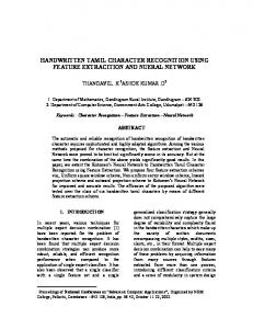
Table 1. Number of features Nbest of the best selected individual for different values of C. Mean number of selected features over 20 runs Nmean and standard deviation σN are also shown. C
Nbest
Nmean
σN
0.8 1 1.2 1.3 1.5 2
176 122 91 75 48 23
163.5 104.05 72.3 54.6 37.85 15.85
25.85 8.03 8.19 9.38 5.81 3.87
GA-based feature selection method, we have performed six experiments using different values for the constant C in equation 1. For each experiment, 20 runs of the GA have been executed with different initial populations, in order to reduce the effects of the stochastic fluctuations due to the randomness of the search. At the end of a run, the best individual found by the GA has been selected. The results are summarized in Table 1, where we have reported, for each experiment, the value of the constant C, the number of features relative to the best individual selected during the 20 runs, the mean number of features over the 20 runs and the standard deviation.
Experimental Results and Discussion
The proposed approach has been tested by using the Multiple Features Data Set available at the UCI Machine Learning Repository [1]. It contains 2000 instances of handwritten digits, 200 for each digit, extracted from a collection of Dutch utility maps. Data are described by using six different sets of features, for a total of 649 features. Each set of features has been used to describe all handwritten digits, and such descriptions have been arranged in a separate dataset. This implies 3
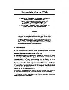
By comparing Table 3 and Table 2, it can be seen that the best recognition rates obtained with every classifier by using the feature subsets selected by our method, are always higher than those obtained by the same classifiers on each single dataset. Moreover, such results are obtained using a much smaller number of features. This highlights that our method is effective in selecting the most discriminant features among the available ones. E. g., a subset of 48 suitably selected features, among the whole set of 649, is sufficient for the MLP classifier to get 98% recognition rate, against 96.46% with 240 features. In practice, it is up to the end user to choose a compromise between feature number and achievable recognition rate, the former implying a higher computational cost. Let us note that, in case of LVQ and KNN classifiers, the best recognition rates are only slightly improved, but they are obtained by using 23 features instead of 240.
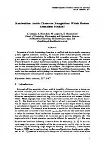
Table 2. Classification results obtained on each of the 6 datasets by using the three considered classifier architectures. The number of features included in each dataset is also shown. Best results are bold. Dataset
# Feature
MLP
LVQ
K-NN
DS1 DS2 DS3 DS4 DS5 DS6
216 76 64 6 240 47
95.85 78.69 94.38 71.46 96.46 82.15
93.92 77.23 92.31 70.77 96.23 77.46
94.85 79.31 93.69 70.77 96.69 79
References
Table 3. Number of features selected by our method among the whole set of 649 features, and corresponding recognition rates, for different values of C. C
Nbest
MLP
LVQ
KNN
0.8 1 1.2 1.3 1.5 2
176 122 91 75 48 23
98.54 98.31 98.46 98.15 98 96.69
94.92 95.62 95.92 95.08 95.46 96.54
95.77 96.00 95.77 96.08 96.23 97.15
[1] R. Duin. UCI machine learning repository. http://archive.ics.uci.edu/ml/machine-learningdatabases/mfeat/. [2] D. E. Goldberg. Genetic Algorithms in Search Optimization and Machine Learning. Addison-Wesley, 1989. [3] I. Guyon and A. Elisseeff. An introduction to variable and feature selection. J. Mach. Learn. Res., 3:1157– 1182, 2003. [4] C. Hung, A. Fahsi, W. Tadesse, and T. Coleman. A comparative study of remotely sensed data classification using principal components analysis and divergence. In Proc. IEEE IntlConf. Systems, Man, and Cybernetics, pages 2444–2449, 1997. [5] J. L. I.S. Oh and C. Suen. Analysis of class separation and combination of class-dependent features for handwriting recognition. IEEE Trans. Pattern Analysis and Machine Intelligence, 21(10):1089–1094, October 1999. [6] M. Kudo and J. Sklansky. Comparison of algorithms that select features for pattern recognition. Pattern Recognition, 33(1):25–41, 2000. [7] J.-S. Lee, I.-S. Oh, and B.-R. Moon. Hybrid genetic algorithms for feature selection. IEEE Trans. Pattern Anal. Mach. Intell., 26(11):1424–1437, 2004. [8] M. Martin-Bautista and M.-A. Vila. A survey of genetic feature selection in mining issues. In Proc. 1999 Congress on Evolutionary Computation (CEC99), pages 1314–1321, 1999. [9] S. Puuronen, A. Tsymbal, and I. Skrypnik. Advanced local feature selection in medical diagnostics. In Proc. 13th IEEE Symp. Computer-Based Medical Systems, pages 25–30, 2000. [10] J. Yang and V. Honavar. Feature subset selection using a genetic algorithm. IEEE Intelligent Systems, 13:44–49, 1998.
For the sake of comparison, we have considered three different classifier architectures: two neural networks, namely a Multi Layer Perceptron (MLP) and a Learning Vector Quantization (LVQ), and a K–Nearest Neighbor (KNN). Each architecture has been used for implementing 6 different classifiers, one for each of the 6 datasets previously introduced and each one trained by using the samples of the corresponding TR. The results obtained by each classifier on the corresponding TS are summarized in Table 2. Finally, each considered classifier architecture has also been used with the dataset DS. For every architecture, we implemented 6 classifiers, one for each of the feature sub–spaces selected by our method. Each subspace has been obtained for a different value of the constant C. Each classifier has been trained and tested by using respectively the projections of TR and TS in the corresponding feature sub–space. The results are summarized in Table 3. 4