Workflow View Definition, and Workflow Normalization based on. Petri Nets. Victor Pankratius ... 76128 Karlsruhe, Germany. Email: {pankratius, stucky}@aifb.uni-karlsruhe.de ... world which is automated by computers. Through- out the paper ...
A Formal Foundation for Workflow Composition, Workflow View Definition, and Workflow Normalization based on Petri Nets Victor Pankratius
Wolffried Stucky
AIFB Institute University of Karlsruhe 76128 Karlsruhe, Germany Email: {pankratius, stucky}@aifb.uni-karlsruhe.de
Abstract In retail information systems it is common practice to subsume the data of products into product groups, which offers organizational advantages for example when new branches are opened, because they are assigned product groups instead of single products. Inspired by this approach, this paper focuses on business processes and proposes the usage of workflow modules stored in a workflow warehouse, which represent reusable, standardized components that are used to build more complex workflow models. In particular, the paper provides a formal foundation for such compositions in form of a workflow algebra based on Petri nets, which has similar operators known from relational algebra in databases. In addition, the need for a concept of workflow normalization is presented, which arises during the composition of workflow modules. Finally, it is shown how the algebra can also be applied in the context of Web service composition. Keywords: Relational Data Model, Relational Algebra, Petri Nets, Workflow Composition, Workflow View Definition, Workflow Normalization, Petri Net Algebra, Web Services 1
Introduction
The multitude of available products that are to be managed by retail information systems (e.g., in supermarkets) has lead to the creation of so-called product groups, which represent sets of particular products (e.g., meat or dairy products). Product groups ease organizational tasks, especially when new branches are opened, because the products to be sold need not be chosen one by one. In addition, product groups represent a standardized range of products available in all branches, thus easing administrative and logistic tasks. Inspired by this approach, this paper takes a closer look at business processes and workflows in such scenarios. Similar to product groups which are a set of products, we use the term workflow modules to denote sets of interrelated activities. We regard a workflow as the part of a business process in the real world which is automated by computers. Throughout the paper Petri nets will be used to model workflows (Petri 1962, Aalst 1996). In addition, this paper draws the attention to applications where predefined, standardized workflow models need to be combined to c Copyright °2005, Australian Computer Society, Inc. This paper appeared at the Second Asia-Pacific Conference on Conceptual Modelling (APCCM2005), University of Newcastle, Newcastle, Australia. Conferences in Research and Practice in Information Technology, Vol. 43. Sven Hartmann and Markus Stumptner, Ed. Reproduction for academic, not-for profit purposes permitted provided this text is included.
create new workflow models. As a practical example, one might think of supermarkets or automotive manufacturers opening new branches which usually have very similar activities. To a large extent, workflow models for different branches may be identical, but often some minor modifications need to be done in order to account for the peculiarities of particular locations. In order to take advantage of economies of scale also on a modelling level by combining predefined workflow models, a precise notation is needed which can be used as a basis for composition languages. The focus of this paper are three related aspects of this composition problem: 1) to provide a formal notation for such compositions in form of a workflow algebra based on Petri nets, which allows to express the creation of a workflow model from other models using an algebraic notation with operators similar to those known from relational algebra in databases. 2) The paper also takes the opportunity to propose a definition of workflow views using the workflow algebra, which is more general than the definitions currently found in the literature (Avrilionis & Cunin 1995, Chiu, Cheung, Till, Karlapalem, Li & Kafeza 2004). 3) Continuing in the composition context, it is shown that the composition problem is not easily solved by a “copy & paste” approach, because a careless design of workflow models using compositions of smaller modules may introduce unwanted properties such as redundancies and other anomalies in the resulting model. To tackle this problem, the need for a notion of workflow normal forms is discussed.
N1: put_in_storage p2:processed_ goods
Handle Complaints
p4:stored_ goods
t2:store_ t1:find_ goods location p1:incoming_ p3:location_document goods N2: receipt_of_goods p2:receipt_ document
t2:quality_ control
Branch 1
N3: place_order p2:completed_form p1:order form
t1:complete_ t2:send_ form form
p4: checked_ goods p4:order_acknow t1:quantity_ p3:goods_ -ledgment p3:goods control qty_checked
p1:goods
Workflow Model 1 WFMS
Workflow Model n WFMS
Branch n
Workflow Warehouse
Workflow Designer
Business Analyst
Figure 1: Workflow Composition Scenario. Figure 1 shows a practical scenario in which a repository, which we call workflow warehouse, is used
to store predefined workflow modules. The workflow modules in such a warehouse are created and annotated with metadata by workflow designers. Business analysts verify and validate the models and make sure that they conform to business practices. The created workflow models represent general reference models for small problem domains (e.g., receipt of goods, handling of complaints, etc.). When a branch is opened, a specific workflow model has to be created that is tailored to the requirements of that branch. However, because of similar requirements of branches, some of the predefined workflow modules can be combined to form an initial model that is subsequently changed. After completion, the model is used in a local Workflow Management System (WFMS) which provides each participant with the right application, the right data, the right inputs at the right time (Georgakopoulos, Hornick & Sheth 1995). Similar to our workflow warehouse, the notion of a process warehouse or repository already exists (Nishiyama 1999, Gruhn & Schneider 1998). The focus, however, is more on a general information source for software process improvement. In the workflow literature, workflow patterns have already been developed (Aalst, Hofstede, Kiepuszewski & Barros 2000). By contrast, such patterns are more abstract than our workflow modules, because they describe elementary workflow operations in a general way (e.g., sequence, synchronization, etc.). In our approach, workflow modules are targeted at particular problem domains and represent more complex workflows that are created for straight reuse. Based on workflow patterns, it has also been shown that Petri nets have advantages over process algebras (Best, Devillers & Koutny 1998) like π-calculus (Milner 1999, Aalst 2003). For example, Petri nets are state-based instead of event-based (important for the expressive power), they have formal semantics despite their graphical nature, and many analysis techniques are available (Aalst & Hofstede 2002). Although various transformations have already been defined for Petri nets (Baumgarten 1996, Desel & Oberweis 1996), the formalizations in general do not allow to express such transformations as precise equations or do not focus on analogies to the relational model. Other approaches like Model Management (Bernstein, Halevy & Pottinger 2000), graph grammars (Rozenberg 1997), or algebraic approaches of graph transformation (Corradini, Montanari, Rossi, Ehrig, Heckel & L¨owe 1997) are too general to be used in the workflow problem domain right away. Nevertheless, our proposal is related to these approaches from a general point of view. The paper is organized as follows. We recapitulate some terms of the relational data model in Section 2. Some basic definitions for Petri nets which are used throughout the paper are introduced in Section 3. A workflow algebra based on Petri nets is presented in Section 4. The applications of the algebra to view definitions on workflows are presented in Section 5. Section 6 introduces the notion of workflow normal forms. Some applications of the algebra to Web services are shown in Section 7. Finally, we discuss the results and mention some aspects for future work. 2
The Relational Data Model
In the Relational Data Model (Codd 1970), data in a database is organized in “tables”. Each “table” has a set of attributes A = {a1 . . . an } with domains dom(ai ), and is described using the mathematical concept of a relation R which is a subset of the cartesian product of the attribute domains, i.e., R ⊆ dom(a1 ) × . . . × dom(an ). A “row” r in a rela-
tion (other than the header row which contains the attribute names) is referred to as a tuple, denoted as r ∈ R : r = (r1 , . . . , rn ). Conceptually, relational algebra is used to construct new relations that contain tuples satisfying some given properties, using other relations. This is done using a few basic operators like selection (σ, used to select a subset of tuples satisfying a given condition), projection (π, picks only specified attribute columns from a relation), join (./, used to combine related tuples from two relations into one single tuple), union (∪, includes all tuples from two compatible relations into one relation without duplicates), and set difference (\, used to include all tuples that are in one of two compatible relations, but not in the other). Furthermore, there are several types of join. For example, the theta-join is a join which allows to specify a join condition, whereas the natural join of two relations pairs only those tuples which agree in the attributes common to both relations (i.e., attributes that have the same name in both relations). Other operators, like for example, intersection, can be constructed by using the elementary operators mentioned before. Expressions of relational algebra can be applied to atomic operands (i.e., relations) or other expressions. Furthermore, all operands and results of expressions can be treated as sets. For further details and extensions we refer to (Garcia-Molina, Ullman & Widom 2002). 3
Petri nets
In analogy to database systems, we want to consider Petri nets as as a “counterpart” to relations in the relational data model. Definition 1 A Petri net N = (P, T, F ) is a directed bipartite graph consisting of a finite set of places P , a finite set of transitions T with P ∩ T = ∅, P ∪ T 6= ∅, and a flow relation F that represents a set of directed arcs F ⊆ (P × T ) ∪ (T × P ), going from places to transitions or transitions to places. ¤ Definition 2 In a Petri net with n places, each place p ∈ P may contain zero or more tokens. Let xi ≥ 0 denote the number of tokens assigned to a place pi . A marking is an n-vector of the form M0 : (x1 , . . . , xn ) which shows the number of tokens assigned to each place pi . A Petri net N with an initial marking M0 is denoted (N, M0 ). ¤ As stated above, it is not allowed to connect nodes of the same type. Furthermore, we assume each place or transition to have a name (e.g., “p1” ) and a label (e.g., “goods”). However, names and labels will be omitted from the formalism, since they would introduce unnecessary complexity for the following argumentations. The set of places with a connection to a transition t are denoted •t and called input places (or pre-set) of t, whereas the set of places which are being connected starting from t via a directed arc are called output places (or post-set) of t, denoted t•. The sets of transitions for a place p, •p and p•, are defined accordingly. In a Petri net, places are passive, and transitions are active components which may change the state of places, according to firing rules. A transition is said to be enabled, if each of the input places contains at least one token. An enabled transition may fire, i.e., it decreases the number of tokens in all input places by one and increases the number of tokens in all output places by one. Transitions can be interpreted as workflow tasks that have to be performed. On the other hand, places can be interpreted as repositories which store tokens (i.e., objects) that are manipulated by tasks. If places contain one token, they can also be interpreted as conditions which evaluate to
true or false. Finally, tokens represent artifacts that have been created by tasks using some input. Sometimes tokens are also referred to as “cases”, because they may represent real-world entities like products or work assignments which progress through the workflow process (Aalst & Hee 2002). The term workflow instance is used to denote a copy of a workflow graph (i.e., the Petri net) created for execution, together with the associated cases. Various extensions to Petri nets have been proposed, like for example higher-order Petri nets (Peterson 1977, Murata 1989, Aalst & Hee 2002), in which a place or transition can also be hierarchically refined using a subnet. We will give further details throughout the paper. Furthermore, the workflow models in our workflow repository represent reference models without associated cases, and we will only consider Petri nets without tokens in the following. Thus, the paper focuses on the analysis of the structure of workflows, not on their dynamic properties. 4
include the places and transitions that are connected by arcs in F 0 into P 0 and T 0 , respectively. Furthermore, we want to use the following shorthand notations given p ∈ P, ti ∈ T, p• = {t1 , . . . , tn } with all ti different: (p, ∗) = (p, t1 ), (p, t2 ), . . . , (p, tn ) Accordingly, we use (∗, p), (t, ∗) and (∗, t). For example, for the Petri net N in Fig. 2a), the expression N 0 = σ{(T ask2,∗),(∗,T ask2)} (N ) returns the highlighted net. Note that it is not allowed to select just one place or transition, since there is no workflow with just one element. We mention that there are other ways to extend the workflow selection operator (e.g., using path expressions, etc.). However, such extensions can be expressed using the definition presented above. Difference The workflow difference operator (\) can be used to “delete” a subnet N 0 from a given Petri net N , which results in a new net N 00 , i.e.,
A Workflow Algebra
We now investigate the possibilities to modify and construct new Petri nets from given Petri nets. We introduce an approach which is inspired by operators known from relational algebra in databases. This approach should also show possible connections between the areas. Similar to relational algebra, we define the operators selection, projection, join, union, and difference for Petri nets. The proposed algebra is closed in that each of the operators applied to one or more Petri nets results again in a Petri net. The advantages of such an algebraic notation are that a series of compositions or other transformations of workflow models can be precisely written down using a single expression. Furthermore, the algebra could represent a basis for the development of programming languages for the composition of workflow models or Web services. Throughout the paper, we will use the following general notations: Given Petri nets N = (P, T, F ), N 0 = (P 0 , T 0 , F 0 ) a) π1 (F ) := {x|∃y : (x, y) ∈ F } b) π2 (F ) := {y|∃x : (x, y) ∈ F } c) N 0 ⊆ N :⇔ N 0 is a subnet of N :⇔ P 0 ⊆ P, T 0 ⊆ T, F 0 = F ∩ ((S 0 × T 0 ) ∪ (T 0 × S 0 )) In a) and b), π1 and π2 are defined to choose the first and the second element of a tuple in F . In c), a shorthand notation for a subnet is defined. Selection We interpret the flow relation F as a database relation which contains a set of pairs representing directed arcs. The arcs start in a place (transition) given by the first element of a tuple and end in a transition (place) specified by the second element of a tuple. In principle, we want the selection operator to select a set of directed arcs from a Petri net together with the places and transitions that they connect, and thus produce a new Petri net. More precisely: Definition 3 (selection) Given a Petri net N = (P, T, F ) and a set of pairs S representing the arcs to be selected from N , we define the workflow selection operator σS (N ) as a transformation that produces from N a net N 0 = (P 0 , T 0 , F 0 ) with F 0 := F ∩ S P 0 := P ∩ (π1 (F 0 ) ∪ π2 (F 0 )) T 0 := T ∩ (π1 (F 0 ) ∪ π2 (F 0 )) ¤ In F 0 , all directed arcs from F are included that are specified in the selection set S. π1 and π2 are used to
Definition 4 (difference) Given a Petri net N = (P, T, F ) and a subnet N 0 ⊆ N with N 0 = (P 0 , T 0 , F 0 ). The difference N \ N 0 is a transformation that produces from N, N 0 a net N 00 = (P 00 , T 00 , F 00 ) with P 00 T 00 F 00
:= P \ P 0 := T \ T 0 := F ∩ ((P 00 × T 00 ) ∪ (T 00 × P 00 )) ¤
In the definition above, the arcs going from the given net N to the subnet N’ are also deleted. Figure 2b) shows an example for N 00 = N \ N 0 with N and N 0 taken from Fig. 2a). Projection The idea behind projection in context of a workflow is to find a subnet of a Petri net which has only places or transitions on its “border” to the rest of the net, and substitute it by a single place or transition, respectively. Although similar maps are known in the Petri net literature (Reisig 1992, Baumgarten 1996), we want to keep the database perspective and the term “projection” for this operator. Thus, we introduce two projection operators which project a subnet either on a place or on a transition. More precisely, we look at a Petri net N = (P, T, F ) and a subnet N 0 ⊆ N , with N 0 = (P 0 , T 0 , F 0 ). Furthermore, the set B (standing for “border”) will denote the set of places and transitions of the subnet N 0 , which are connected with the rest of the net N , i.e., B(N 0 , N ) = {x ∈ P 0 ∪ T 0 |(x • ∪ • x) \ (P 0 ∪ T 0 ) 6= ∅} with x• and •x applied with regard to N . Furthermore, we will use the terms place-bordered subnet and transition-bordered subnet to denote a subnet whose set B contains only places or transitions, respectively. Definition 5 (place projection) Given a Petri net N , a place-bordered subnet N 0 ⊆ N , and a place pnew ∈ / P (used to substitute the subnet). We define the place projection operator πP (B→pnew ) (N ) as a transformation that produces from N, N 0 a net N 00 = (P 00 , T 00 , F 00 ) with P 00 := (P \ P 0 ) ∪ {pnew } T 00 := T \ T 0 F 00 := Φ(F \ F 0 ),
N:
N'':
N:
Result 1a
Result 3
Result 1a Task3 Task1
Input 1
Result 1b
Task3
Result 1a
Result 2a
Task2
Task1
Input 1
a) Selection: N'=
Task 2
Task 2
(N)
b) Difference: N''= N \ N'
{(Task2,*), (*,Task2)}
N:
N'':
Input 1
Result 1
Result 1b
N'
N:
N'
Task 1b
Result 3
Result 2b Input 2
N'': Task 1
Task 1
N'':
Task 1
Input 1
N''=
P ({Result1a, Result1b}
N:
Task 1
Result 1a
Task 1
Task 1b Result
N' Task 1
Result 1
Task 4
Task 4
e) Place Join: N'' = N
d) Transition Projection: N''= T ({Task1a, Task1b} Task1) (N) N'':
P (Result1, Result2)
(N')
Task 1
Task 2 Result 1
Result 1
Task 3
Result
Input 2
Input 2
Task 2
Result 2
Task 3
(N)
N'':
N' Result 1
Result1)
Input 1
Input 1
Task 2
Task 1a
c) Place Projection:
Result 2
Result 2
f) Transition Join: N'' = N
T (Task1, Task2)
(N')
N'':
N Input 1
Result 3
Task3
Result 1a
N
Task1
Result 1a Task3
Result 3
Result 1b
Result 2a
Input 1 Task1 Result_1b
Result 2a
Task2
Task2
Result 2b Input 2
g) Theta Join: N" = N
Result 2b
N'
N'
Input 2
{(PN.Task1, PN'.Result_1b)}
(N')
h) Union: N" = N
N'
Figure 2: Operations from relational algebra defined for workflows which are represented as Petri nets. Φ(F ) = {ϕ(x, y)|(x, y) ∈ F } ϕ(x, y) =
(
(x, y) if (x, pnew ) if (pnew , y) if
0
0
x, y ∈ (P ∪ T ) \ (P ∪ T ) y ∈ B(N 0 , N ) x ∈ B(N 0 , N ) ¤
In the definition above, the function ϕ is used to relocate arcs (which are coming from “outside” into the subnet or which go from the subnet to the “outside”) to the new place. Similarly, for a transition-bordered subnet N 0 ⊆ N , we define the transition projection operator πT (B→tnew ) (N ). For example, Fig. 2c) and 2d) show the results for the expressions: N 00 = πP ({Result1a,Result1b}→Result1) (N ) N 00 = πT ({T ask1a,T ask1b}→T ask1) (N ) The inverse operation of a projection – the substitution of a place or transition by a subnet with either only places or transitions on the border – is also a useful operation to hierarchically design workflow models. Such an operation is known as refinement in the Petri net literature (Reisig 1992). In our algebra, we can express the semantics of such an operator by using the difference and the join operator presented next.
Join In analogy to databases, we introduce two types of join to combine Petri nets: natural join (referred to as join in the following) and theta join. Natural Join. Similar to the natural join operator in databases, the natural join operator for Petri nets can be used to create a new Petri net from two given Petri nets, which have both a place-bordered or transition-bordered subnet regarded as “common”. Because we have shown that the projection operator can be used to replace such subnets by places or transitions, we define the join operator for common places or transitions, and not for subnets (see Fig. 2). Again, two natural join operators are needed: one for joining on places (that will be called place join, denoted as ./P ) and one for joining on transitions (called transition join, denoted as ./T ). Definition 6 (place join) Given two Petri nets N = (P, T, F ), N 0 = (P 0 , T 0 , F 0 ) with P ∩ P 0 = ∅, T ∩ T 0 = ∅, a set of pairs J = {(p1 , p01 ) . . . (pn , p0n )} with pi ∈ N and p0i ∈ N 0 , which represent the places on which N and N 0 will be ”glued” together. The place join N ./P J (N 0 ) is a transformation that produces from N, N 0 a new Petri net N 00 = (P 00 , T 00 , F 00 ) with
The result of the union operator can express for example that N and N 0 are workflows which are executed concurrently. In contrast to relations in databases, the Petri nets do not have to be “compatible”. Figure 2h) shows an example for the expression:
τ2 (J) := {y|∃x : (x, y) ∈ J} P 00 := (P ∪ P 0 ) \ τ2 (J) T 00 := T ∪ T 0 F 00 := Φ(F ∪ F 0 ) (x, y) (x, y) ϕ(x, y) = (x, pi ) (pi , y)
if if if if
N 00 = N ∪ N 0 .
x, y ∈ P ∪ T x, y ∈ (P 0 \ τ2 (J)) ∪ T 0 y = p0i ∈ τ2 (J) x = p0i ∈ τ2 (J) ¤
The two nets are joined together on the places specified in J. Then, the function ϕ is used to “relocate” arcs. The definition for the transition join operator N ./T J (N 0 ) is similar and we omit it here. Figure 2e) and 2f) depict examples for the expressions:
Example As an example for the usage of the algebra, we assemble a custom workflow X using the modules shown in Fig. 1 inside the workflow warehouse. The result of the following expression is shown in Fig. 3: X = N 1 ./P {(N 1.p1,N 2.p3)} (N 3 ./P {(N 3.p4,N 2.p2),(N 3.p3,N 2.p1)} (σ{(p1,t1),(p2,t1),(t1,p3))} (N 2)))
N 00 = N ./P {(Result1,Result2)} (N 0 ) and N 00 = N ./T {(T ask1,T ask2)} (N 0 ). The semantics behind a place join is that places of different nets are merged to more centralized repository of results. This type of join can be used to model mutual exclusion in workflows. In the Petri net community, such a composition is called fusion (Desel & Oberweis 1996). The semantics of a transition join operation is that tasks of different nets are merged together to a new task, which can only be performed if all inputs are available. Therefore, the transition join introduces synchronization. This is why the Petri net community refers to such transformations as synchronization (Desel & Oberweis 1996). Theta Join. The theta join allows to combine Petri nets N and N 0 and add additional arcs between them, specified in a connection set. This way, other “branches of execution” described in N 0 can be added, which were previously not included in N . Definition 7 (theta join) Given two Petri nets N = (P, T, F ) and N 0 = (P 0 , T 0 , F 0 ) with P ∩ P 0 = ∅, T ∩T 0 = ∅. The theta join N ./connection set (N 0 ) with connection set 6= ∅ is a transformation that produces from N, N 0 a new net N 00 = (P 00 , T 00 , F 00 ) with connection set ⊆ {(P × T 0 ) ∪ (T × P 0 )∪ ∪(P 0 × T ) ∪ (T 0 × P )} 00 P := P ∪ P 0 T 00 := T ∪ T 0 F 00 := F ∪ F 0 ∪ connection set
X:
order_acknowledgment
completed_ form
order complete_ form form
send_ form
stored_goods
incoming_goods find_ location
goods quantity_ control processed_ goods store_goods
location_ document
Figure 3: Example for a workflow composition using the workflow algebra. First, a selection is made from the receipt of goods workflow (N2) without the quality control. Then, the place order workflow (N3) is joined, and the places for goods (N 3.p3 and N 2.p1) and order acknowledgement (N 3.p4 and N 2.p2) are joined together, and the arcs are relocated. Finally, the put in storage workflow N 1 is joined, and the places N 1.p1 and N 2.p3 are glued together. Given Petri nets: N = (P, T, F ), N 0 = (P 0 , T 0 , F 0 ), N 00 = (P 00 , T 00 , F 00 ) Properties:
¤ The theta join operator is able to connect transitions (places) from one net with places (transitions) of the other net and vice versa. An example for N 00 = N ./{(N.T ask1,N 0 .Result1b)} (N 0 ) is depicted in Fig. 2g).
1)
N ∪ N0 = N0 ∪ N
2)
For S1 ⊆ F, S2 ⊆ F, S1 ⊆ S2 : σS1 (σS2 (N )) = σS1 (N )
3)
For S ⊆ (F ∪ F 0 ): σS (N ∪ N 0 ) = σS (N ) ∪ σS (N 0 )
4)
For S1 , S2 ⊆ F : σS1∪S2 (N ) = σS1 (N ) ∪ σS2 (N )
5)
For N 00 ⊆ N 0 ⊆ N : B 00 = B(N 00 , N 0 ), B 0 = B(N 0 , N ), and N 00 , N 0 place-bordered subnets:
Union In the context of workflows and Petri nets we regard a union of two Petri nets N and N 0 as the union of their places, transitions, and flow relations. Definition 8 (union) Given two Petri nets N = (P, T, F ) and N 0 = (P 0 , T 0 , F 0 ). The union N ∪ N 0 is a transformation that produces from N, N 0 a new net N 00 = (P 00 , T 00 , F 00 ) with P 00 := P ∪ P 0 T 00 := T ∪ T 0 F 00 := F ∪ F 0 ¤
πP
(N )) (B 0 →p0new ) (πP (B 00 →p00 new ) πP
6)
=
(B 0 →p0new ) (N )
For p2 ∈ P 0 , {t1 . . . tn} = •p2, {t10 . . . tn0 } = p2•: N ./P {(p1,p2)} (N 0 ) = N ./{(t1,p1)...(tn,p1),(p1,t10 )...(p1,tn0 )} ( (N 0 \ σ{(p2,∗)} (N 0 ))∪ (N 0 \ σ{(∗,p2)} (N 0 )) )
Table 1: Properties of the workflow algebra.
We finally point at some properties of the workflow algebra, presented in table 1, and give some brief ideas of the proofs. The commutativity of the union operator which follows from Def. 8 is expressed in (1). Equation (2) states that if a more special selection is made from a selection, the more special selection can be made right away, following from Def. 3. Equation (3) expresses that the selection from a union of two Petri nets can be split up, a result obtained from Def. 3 and 8. In (4) a selection with two unified selection sets can be replaced by two independent selections with one of the selection sets, followed by union of the results. This can also be obtained from Def. 3 and 8. In (5) it is stated that in a situation with two nested, place-bordered subnets, one projection can be omitted. Equation (6) shows that a (natural) place join between two nets N and N 0 on p1 and p2 can be expressed using the theta join, selection, difference, and union operators. The idea is to first select all parts of N 0 except the place p2 and except the arcs to and from that place, using the expression (N 0 \ σ{(p2,∗)} (N 0 )) ∪ (N 0 \ σ{(∗,p2)} (N 0 )). Then, using the theta join, the arcs from the transitions of N 0 pointing to p2 are relocated to p1; the same is done for the arcs going to the post-set of p2. Despite this realization we do not remove the place or transition join operators from the algebra, because they are used frequently. The properties (5) and (6) are similar for transition projection and transition join. Interestingly, we want to mention that if the notation was adapted to the relational data model and relational algebra (e.g., N and N 0 as relations; S, S1 , S2 as conditions), the properties (1), (3), (4), (5) would be similar for relations. The natural join in the relational model can also be expressed using theta join and an additional projection (Elmasri & Navathe 2004). Of course, for a more thorough comparison, further adaptations are needed with respect to the exact notation and the peculiarities of the relational model (e.g., “compatible” relations for union, etc.), which we do not discuss here in more detail. In addition, there are also significant differences to the relational case, as other properties known from relational algebra do not hold in our case. For example, the selection operator has other properties (2). Thus, although the models have many commonalities, it cannot be said that there is an analogy in all respects. Nevertheless, such a close relationship between the models provides new ground for investigations if other concepts from the relational model (e.g., views, normalization) can be applied to workflows and Petri nets. 5
Workflow Views
Originating in the area of databases, views are virtual relations which are derived from existing relations or other views, for example by using relational algebra operators (Elmasri & Navathe 2004). Views are not materialized, and they are typically computed every time a user accesses them. A database user cannot distinguish between a relation or a view. However, data manipulation and update operations on views are restricted, because there may be ambiguities when such operations are mapped back to the original relations. A view definition is useful when the result of several joins of relations is used frequently, or when access to data has to be restricted, so that certain employees should see only some parts of the data. Starting from database views, the need for a view concept on workflows has already been recognized in the literature (Avrilionis & Cunin 1995, Chiu et al. 2004). However, a workflow view is often regarded only as a sub-model of the original workflow
model, thus not directly corresponding to the definition of database views which allow the combination of several relations or views for the definition of a new view, using relational algebra. We therefore propose the usage of our workflow algebra for a more general definition of workflow views. We propose the usage of any expression of our algebra for the definition of a view on workflow models. Such a workflow view is not materialized and will be recomputed every time it is accessed. S: s1: shipping_ centre t1: product_ delivery
t2: put_stock_1
t3: put_stock_2 t5: get_stock_2
t6: sell
View1:
s4: PointOf Sale
s3: stock2
t4: get_stock1
s1: shipping_ centre t1: product_ delivery
s2: stock1
s5: stock
t7: put_stock
Figure 4: Example for a workflow view. As a simple example, let us consider a practical scenario where a manager wants to streamline business processes to make them more efficient. For a discussion with the board of directors, he needs to know the main activities and their interconnections without too many details, based on the workflow model used in the company (e.g., S in Fig. 4), starting from product delivery to storage (he will unexpectedly ask the employees to do this quickly, like all managers do). To solve this problem, View1 can be defined using the expression: V iew1 = σ{(t1,∗),(s1,∗),(∗,s5)} ( π({t2,t3}→t7) (π({s2,s3)→s5} (S))) The view aggregates the places labelled stock1, stock2 and the transitions labelled put stock1, put stock2 from S, and selects only the desired part of the workflow. It should be noted that the “*” in the selection set has a dynamic aspect; if the underlying model was changed in the meantime, e.g., a new place was added in the post-set of t1, it would appear in the view. Thus, if the workflow models are changed frequently due to the adaptation to new requirements, the view always provides up-to-date, customized information. In addition, business analysts often differentiate between core processes which contribute to the core competencies of a company and its competitive advantage, and support processes which provide support for the core business processes. Using views, the current core processes and support processes can be extracted from the company-wide workflow model. Other operations also make sense when applied on workflow views. A union may combine different pieces of workflows or other views to one big overview for the manager. This is very useful to supervise the activities of several projects that run in parallel. Difference may be used to cut execution paths which are not in the focus of the analysis. Joins can be used to present a simplified model of interorganizational workflows. For example, a view for company A shows a simplified model of a manufacturing process in which products are output to a place AO . Another view for company B in the same supply chain uses the products of company A as input to its production process, modelled by a place BI . The general “big
picture” would be obtained by joining the two views on AO and BI . Such an approach can be very useful in Supply Chain Management (SCM) to analyze and streamline processes which are crossing several companies. Furthermore, during mergers & acquisitions of companies, a workflow analysis based on views can also help to find interfaces and integrate the business processes of an acquired company more efficiently. Just like in the database area where operations on views need to be restricted, in workflow views not all combinations of workflows may make sense with respect to the underlying workflow. Since this depends on the specific situation and workflow, such constraints need to be verified by a runtime system. In addition, we mention that workflow views also need to restrict the way tokens are shown in a view, because the firing rules in a view may not conform to the underlying workflows. For example, this may occur in situations where several places are projected onto one single place. However, a solution to this problem is out of scope here, since the focus is on the structure of the workflows (Petri nets without tokens), not the dynamic aspects. Nevertheless, it would be advantageous to show tokens in a view as progress and status indicators. 6
Workflow Normalization
Continuing with the composition scenario shown in Fig. 1 we argue in this section that a notion of normal forms for workflows is needed. As with database relations, a careless design of workflow models using Petri nets can lead to problems. For example, a workflow designer may be tempted to use “copy & paste” functionality of an editing tool (based on our workflow algebra) to copy a module from the workflow warehouse (cf. Fig. 1) and paste it multiple times at different locations in the workflow model he or she is designing for a branch. This introduces anomalies, some of which are similar to those found in relational databases (Elmasri & Navathe 2004): 1. Redundancy. The information contained in the workflow modules is repeated unnecessarily in the workflow model. 2. Update Anomalies. Suppose that a workflow module named “place order” was inserted multiple times at different locations in the workflow model. If suddenly an extension has to be made (e.g., a transition has to be added), the same insertion has to be made in multiple locations (we assume that this change is only needed in that particular workflow model, so that it is not appropriate to modify the global module in the workflow warehouse). If possible, it would be much better to have just one copy of the module in the whole workflow model and thus, only one insertion. 3. Inconsistent Behaviour. In the example above, the workflow designer may forget to make the changes to all copies of the “place order” module in the model. Such inconsistent changes lead to different, unintended workflow behaviour which does not conform to the specifications. The anomalies presented above are definitely undesirable and should be prevented by using a systematic conceptual approach. Although the methodology and the properties may slightly differ in the following from databases, we chose to stick to the term “normalization”, because in our view, the same goal is pursued: a better design that avoids anomalies. In databases, so-called functional dependencies
are analyzed to eliminate some anomalies (Elmasri & Navathe 2004). In our workflow context, we analyze the flow dependencies along with the structure of a Petri net. As in the rest of the paper, we stick to Petri nets without tokens. In analogy to databases, we propose the notion of workflow normal forms for Petri-net-based workflow models. The main intention is to specify criteria for a “good” structure of workflows. Such criteria are also especially useful in business process reengineering projects, in which existing workflow models need to be analyzed and restructured. We point out that our notion of workflow normal forms should not be confused with normalized Petri nets found in the Petri net literature (Tiplea & Tiplea 1998), which denote Petri nets whose weight function and initial and final markings take only values in {0, 1}. Definition 9 (1NF) We define a workflow represented as a Petri net to be in First Normal Form (1NF), if all places or transitions are atomic, i.e. if no place or transition is hierarchically decomposable into sub-workflows. ¤ The 1NF is intended to flatten out hidden subworkflow specifications of a workflow. This is necessary for the identification of redundant flow specifications, and to reveal the real structure of the net. Based on a workflow model in 1NF, further analysis can be done. For this, we first need to introduce some other definitions: Definition 10 (Petri net morphism) Given Petri nets N = (P, T, F ) and N 0 = (P 0 , T 0 , F 0 ). A structure-respecting Petri net morphism is a map ϕ : P × T → P 0 × T 0 in which for every (x, y) ∈ F holds: 1) If (x, y) ∈ F ∩ (P × T ) then either (ϕ(x), ϕ(y)) ∈ F 0 ∩ (P 0 × T 0 ) or ϕ(x) = ϕ(y) and 2) If (x, y) ∈ F ∩ (T × P ) then either (ϕ(x), ϕ(y)) ∈ F 0 ∩ (T 0 × P 0 ) or ϕ(x) = ϕ(y). Definition 11 (isomorphism) A bijective map ρ : P ∪ T → P 0 ∪ T 0 that preserves the structure of places and transitions is called an isomorphism, i.e., the map of the net N = (P, T, F ) onto N 0 = (P 0 , T 0 , F 0 ), is an isomorphism if ∀x, y ∈ P ∪ T : (x, y) ∈ F ⇔ (ρ(x), ρ(y)) ∈ F 0 . Two nets are called isomorphic if there is an isomorphism from one net onto the other. ¤ In general, Def. 10 provides a mapping from a source net to a target net in which some structural properties of the source net are preserved. The term “morphism” is generally used for the mapping as well as for the resulting net. Definition 11 (which is also a morphism) can be used to find identically structured subnets inside a workflow model. Definition 12 (2NF) A workflow represented as a Petri net in 1NF is in second normal form (2NF) if there are no multiple occurrences of isomorphic subnets with identically labelled places or transitions. ¤ In Sect. 3 we assumed that a place or transition can have a name (e.g., “p1”) and a label (e.g., “order form”). Definition 12 demands that there should be no subnets with identical structure and identical labels (even though the names of labels or transitions may be different, e.g. fill out
fill out p1
t1
order form
p2
completed form
vs.
p5
t7
order form
p9
completed form
). If a workflow model N is not in 2NF, there must be multiple copies (e.g., N10 , N20 ) of a subnet N 0 at different
N: N'
A a)
B
N1'
C
N2'
D
t1
pi
pO
t2
pi1 pO1
t3
pi2
pO2
t4
p1
ti
tO
p2
ti1 tO1
p3
ti2
tO2
p4
Y:
y.N'
b)
y.t1 y.p1
pi
pO
ti
tO
E
y.t2 y.t3 y.t4
E
Figure 5: Example for normalization. locations in the model N . This situation is suspect, since it points to conceptual errors which can be of two types: 1) N10 , N20 are actually meant to be the same as N 0 . In this case, the workflow model has to be restructured to contain N 0 only once. 2) N10 , N20 may occur in another context, and therefore be different, which justifies their existence. However, in this case the labels have to be renamed properly to reflect this different context (e.g., place labels “completed form” to “completed order form” and “completed goods receipt form”, respectively – reflecting different forms). Both actions lead to a workflow in 2NF. Let us consider the case 1) where a workflow N needs to be restructured, depicted in general in Fig. 5a). In the figure, multiple copies (N10 , N20 ) of the subnet N 0 occur multiple times in the workflow model (we assume that places and transitions have different names, but identical labels). Since the exact structure of N 0 is not of interest, no arcs are shown inside. The borders (see Sect. 4) connecting the copies of N 0 with other parts of the net consist of input and output places and transitions {pi , po , ti , to }. Each of these places and transitions represent a projection of a more complex subnet. The copies of N 0 are connected to other nets A, B, C, D, whose representations are also simplified assuming their border contains places as well as transitions, which are projected on one place and transition only. To avoid anomalies (e.g., when N 0 is updated) the structure of the workflow model has to be changed to contain N 0 only once. In principle, this can be accomplished using structurerespecting morphisms. An example for such a morphism is the folding operation: Definition 13 (folding) Given two Petri nets N = (P, T, F ) and N 0 = (P 0 , T 0 , F 0 ). The folding operation is a surjective map ψ : P ∪ T → P 0 ∪ T 0 , where ψ(P ) ⊆ P 0 , ψ(T ) ⊆ T 0 , and (x, y) ∈ F ⇒ (ψ(x), ψ(y)) ∈ F 0 ¤ The folding operation maps places from a net N to places of N 0 and transitions from N to transitions of N 0 and preserves the flow dependencies. The operation is useful to “fold” identically structured parts of a workflow model on top of each other and thus reduce their multiple occurrence (redundancy). In the Petri net literature (Baumgarten 1996), folding is compared to the creation of procedures and procedure calls in programming languages. As an example, Fig. 5b) shows how the folding operation can be applied to obtain a new workflow model with N 0
occurring only once. Each place and transition of the net N 0 is mapped to those of y.N 0 ; the places p1 . . . p4 are mapped onto y.p1 that now represents an input/output repository for y.N 0 . The mapping of the transitions t1 . . . t4 has to be done with care. They cannot be mapped altogether on y.t1, since they may represent different tasks outside N 0 . In addition, after mapping t2 . . . t4 onto y.t2 . . . y.t4, the firing order t2 < t3 < t4, which represents a sequential processing, is lost. The firing order can be preserved by adding constraints, for example by using predicates or other constructs like inhibitor arcs (Peterson 1977). In practice, several isomorphic subnets with identically labelled places or transitions may occur at different levels of aggregation. In such cases, the largest isomorphic subnets occurring multiple times should be identified first (e.g., using clustering (Keller 2003) or other algorithms (Kuramochi & Karypis 2004)) and the discussed procedure should be applied. The same can be done recursively with the subnet, until the 2NF of the workflow model is reached. We point out that a “good” structure of a workflow model may also depend on the semantics related to labels of places and transitions, which cannot be inferred only by analyzing the structure. Places or transitions with different labels may mean the same. For example, two transitions performing the same task may be labelled “process request” and “work on customer inquiry”. Definition 14 (3NF) A workflow represented as a Petri net in 2NF is in third normal form (3NF) if there are no multiple occurrences of isomorphic subnets with semantically identical labels for places or transitions. ¤ In our view, a workflow designer can be provided with some semi-automatic assistance for detecting such redundancies of places or transitions with different labels meaning the same, for example by using synonym dictionaries and concepts developed for the Semantic Web (Berners-Lee, Hendler & Lassila 2001). This implies additional effort during the design of a workflow module, in which places and transitions may be associated with concepts contained in an ontology (Staab & Studer 2003) that is valid for the whole warehouse. The ontology represents a taxonomy of classes of objects and relations among them – an information that can be used by an inference mechanism to automatically draw conclusions and make propositions to the workflow designer. Finally, we mention that there are also other types of Petri net morphisms, each of which preserve different properties of a Petri net (see (Mikolajczak & Wang 2003) for a comparison), and which also take
tokens and the behaviour of nets into account. Based on different types of morphisms and the dynamic behaviour of Petri nets, further workflow normal forms can be developed. This may be especially beneficial for avoiding situations with deadlocks which may result from the composition process. Behaviour-based workflow normal forms may therefore represent further milestones for quality criteria during workflow composition. Since we concentrate on Petri nets without marking at this time, such an examination is beyond the scope of this paper. 7
Application to Web Services
In this section, we show how the developed concepts of the workflow algebra and workflow views can also be applied in the context of Web services. Web services play an important role in the workflow area, since they are used to implement activities of business processes (Leymann, Roller & Schmidt 2002). Web services are independent software components that use the Internet as a communication and composition infrastructure. Building on a standardized stack of protocols, Web services provide a serviceoriented view and abstract from specific computers (see (Casati & Dayal 2002) for details). Web service composition is used to create higher-level services based on other Web services, e.g., a travel agent may compose a hotel reservation and airline ticket service to offer a new service. In this context, the concept of orchestration is targeted at the interaction between Web services at message level and focuses for example on the execution order of interactions. Choreography refers to the overall message exchange between all Web services that participate in a collaborative exchange, and is for example directed towards exception handling or transactions. The strict separation between orchestration and choreography is blurring as various languages and standards have been developed: Business Process Execution Language for Web Services (BPEL4WS), Web Services Choreography Interface (WSCI), Business Process Management Language (BPML), XLANG, Web Services Flow Language (WSFL). A detailed comparison is given in (Peltz 2003, Aalst, Dumas & Hofstede 2003). Using the workflow algebra introduced in Sec. 4, we can describe the creation and composition of services on a conceptual level. We assume that the behaviour of a Web service is described by an associated Petri net, which has one input and one output place. Unlike other Petri-net-based composition approaches (Hamadi & Benatallah 2003), we use the algebra not only to join input and output places of available services, but also to construct services from modules in the workflow warehouse (cf. Fig. 1). In this context, we assume that the warehouse contains predefined modules for business processes as well as modules needed for the technical realization of Web services, described as Petri nets. A current problem in the area of Web service composition is that often the exact mode of operation and the “inside” of a Web service used for composition is not known. In many cases, the providers don’t want to reveal such details because of competitive advantages. Such information, however, could be important if a certain quality of service level has to be ensured in a composite service, or to avoid deadlocks with services from other providers. We propose the application of workflow views (cf. Sec. 5) as a compromise, which are derived from the Petri net associated with the service. When a developer requests the Petri net description associated with a service, a view on that Petri net is returned. Using the selection, projection, or difference operators (cf. Sec. 4), the parts that
the provider does not want to reveal to the public may be eliminated. In a more sophisticated scenario, different views with different levels of detail may be computed for different types of (paying) customers. The advantage is that the underlying functionality of the service and the Petri net model are not changed at all, since the view is computed dynamically upon request. 8
Conclusion
This paper addresses problems encountered during the composition of workflow modules. The need for theoretical constructs is motivated by the descriptions of practical scenarios from supermarket chains or automotive manufacturers which use a workflow warehouse to build new workflow models from existing ones. A formal notation (workflow algebra) for the composition of Petri nets is proposed which is inspired by operators known from relational algebra. To a certain extent, the properties of the workflow algebra are similar to those of relational algebra, and interesting relationships are revealed. We expect that users will adapt quickly to languages based on the proposed workflow algebra, due to the popularity of database concepts. Furthermore, using the workflow algebra, the concept of workflow views is extended in such a way that dynamically computed views on workflows may aggregate, eliminate, or combine parts of workflows. In addition, it is shown that a careless modelling and composition of workflow models may lead to unwanted anomalies – some of them similar to databases. Therefore, the need for a notion of workflow normal forms is discussed to tackle this problem. Finally, it is shown that the presented concepts can also be used to describe the creation and composition of Web services which are often used to implement activities of business processes. In this context, workflow views seem to be a promising solution for the delivery of the the internal processing model of a Web service, since they may aggregate or eliminate parts that should not be revealed to the public. This paper also tries to identify potential future directions for workflow and business process management research, in particular with respect to workflow normalization algorithms. In the future, further investigations are needed to connect the results from Petri nets without tokens with Petri nets which contain tokens. In addition, the resulting implications for workflow views and workflow normal forms with respect to dynamic net behaviour have to be analyzed in more detail. Acknowledgements. The first author would like to thank Phil Bernstein for the fruitful discussion at SIGMOD/PODS 2004 in Paris, France. References Aalst, W. (1996), Three good reasons for using a petri-net-based workflow management system, in ‘Proceedings of the International Working Conference on Information and Process Integration in Enterprises (IPIC’96)’, pp. 179–201. Aalst, W. (2003), ‘Pi calculus versus petri nets: Let us eat humble pie rather than further inflate the pi hype’, http://tmitwww.tm.tue.nl/research/patterns/ download/pi-hype.pdf (unpublished discussion paper) . Aalst, W., Dumas, M. & Hofstede, A. (2003), Web service composition languages: Old wine in
new bottles?, in ‘29th EUROMICRO Conference 2003, New Waves in System Architecture, 3-5 September 2003, Belek-Antalya, Turkey’, IEEE Computer Society, pp. 298–307. Aalst, W. & Hee, K. (2002), Workflow Management. Models, Methods, and Systems, MIT Press. Aalst, W. & Hofstede, A. (2002), Workflow patterns: On the expressive power of (petri-net-based) workflow languages., in K. Jensen, ed., ‘Proceedings of the Fourth Workshop on the Practical Use of Coloured Petri Nets and CPN Tools (CPN 2002)’, Vol. 560 of DAIMI, University of Aarhus, Aarhus, Denmark, pp. 1–20. Aalst, W., Hofstede, A., Kiepuszewski, B. & Barros, A. (2000), Advanced workflow patterns, in O. Etzion & P. Scheuermann, eds, ‘Proc. 7th International Conference on Cooperative Information Systems (CoopIS)’, Vol. 1901 of Lecture Notes in Computer Science, Springer-Verlag, Berlin, pp. 18–29. Avrilionis, D. & Cunin, P. (1995), Using views to maintain petri-net-based process models, in ‘Proc. International Conference on Software Maintenance’, pp. 318–326. Baumgarten, B. (1996), Petri-Netze. Grundlagen und Anwendungen (in German), 4th edn, Spektrum Akademischer Verlag. Berners-Lee, T., Hendler, J. & Lassila, O. (2001), ‘The semantic web’, Scientific American . Bernstein, P. A., Halevy, A. Y. & Pottinger, R. (2000), ‘A vision of management of complex models.’, SIGMOD Record 29(4), 55–63. Best, E., Devillers, R. & Koutny, M. (1998), Petri nets, process algebras and concurrent programming languages, Vol. 1492 of Lecture Notes in Computer Science (LNCS), Springer, Berlin. Casati, F. & Dayal, U., eds (2002), Special Issue on Web Services, Vol. 25, IEEE Bulletin of the Technical Committee on Data Engineering. Chiu, D. K., Cheung, S., Till, S., Karlapalem, K., Li, Q. & Kafeza, E. (2004), ‘Workflow view driven cross-organizational interoperability in a web service environment’, Information Technology and Management 5(3-4), 221–250. Codd, E. F. (1970), ‘A relational model of data for large shared data banks’, Commun. ACM 13(6), 377–387. Corradini, A., Montanari, U., Rossi, F., Ehrig, H., Heckel, R. & L¨owe, M. (1997), Algebraic Approaches to Graph Transformation, Vol. 1 of Rozenberg (1997), chapter 3, pp. 163–245. Desel, J. & Oberweis, A. (1996), ‘Petri nets in applied computer science (in German)’, Wirtschaftsinformatik 38(4), 359–367. Elmasri, R. & Navathe, S. B. (2004), Fundamentals of Database Systems, 4th edition edn, Pearson Addison Wesley. Garcia-Molina, H., Ullman, J. D. & Widom, J. (2002), Database Systems. The Complete Book., Prentice Hall, Inc. Georgakopoulos, D., Hornick, M. & Sheth, A. (1995), An overview of workflow management - from process modeling to workflow automation infrastructure, in ‘Distributed and Parallel Databases’, Vol. 3, pp. 119–153.
Gruhn, V. & Schneider, M. (1998), Workflow management based on process model repositories, in ‘Proceedings of the 20th international conference on Software engineering’, IEEE Computer Society, pp. 379–388. Hamadi, R. & Benatallah, B. (2003), A petri netbased model for web service composition, in ‘Proceedings of the Fourteenth Australasian database conference on Database technologies 2003’, Australian Computer Society, Inc., pp. 191–200. Keller, W. (2003), ‘Clustering for petri nets’, Theor. Comput. Sci. 308(1-3), 145–197. Kuramochi, M. & Karypis, G. (2004), ‘An efficient algorithm for discovering frequent subgraphs’, IEEE Transactions on Knowledge and Data Engineering 16(9), 1038–1051. Leymann, F., Roller, D. & Schmidt, M.-T. (2002), ‘Web services and business process management.’, IBM Systems Journal 41(2), 198–211. Mikolajczak, B. & Wang, Z. (2003), Conceptual modeling of concurrent systems through stepwise abstraction and refinement using petri net morphisms., in I.-Y. Song, S. W. Liddle, T. W. Ling & P. Scheuermann, eds, ‘Proc. 22nd International Conference on Conceptual Modeling’, Springer, Chicago, IL, USA, pp. 433–445. Milner, R. (1999), Communicating and Mobile Systems: The π-Calculus, Cambridge University Press, Cambridge, UK. Murata, T. (1989), Petri nets: Properties, analysis and applications, in ‘Proc. IEEE’, Vol. 77, pp. 541–580. Nishiyama, T. (1999), Using a “process warehouse“ concept. a practical method for successful technology transfer., in ‘2nd International Symposium on Object-Oriented Real-Time Distributed Computing (ISORC ’99), May 2-5, 1999, Saint Malo, France’, IEEE Computer Society, pp. 117– 120. Peltz, C. (2003), Web services orchestration. a review of emerging technologies, tools, and standards., Technical report, Hewlett-Packard Company. Peterson, J. L. (1977), ‘Petri nets’, ACM Comput. Surv. 9(3), 223–252. Petri, C. A. (1962), ‘Kommunikation mit Automaten (in German)’, Schriften des Instituts f¨ ur instrumentelle Mathematik, University of Bonn, Germany . Reisig, W. (1992), A Primer in Petri Net Design, Springer Verlag. Rozenberg, G., ed. (1997), Handbook of Graph Grammars and Computing by Graph Transformation, Vol. 1, World Scientific. Staab, S. & Studer, R., eds (2003), Handbook on Ontologies, Springer, Berlin. Tiplea, F. & Tiplea, A. (1998), On normalization of petri nets, in ‘Proc. of the 11th Romanian Symposium on Computer Science ROSYCS’98’, Iasi, Romania.