RC23373 (W0410-079) October 13, 2004 Computer Science
IBM Research Report A Framework for Applying Inventory Control to Capacity Management for Utility Computing Joseph L. Hellerstein, Kaan Katircioglu, Maheswaran Surendra IBM Research Division Thomas J. Watson Research Center P.O. Box 704 Yorktown Heights, NY 10598
Research Division Almaden - Austin - Beijing - Haifa - India - T. J. Watson - Tokyo - Zurich LIMITED DISTRIBUTION NOTICE: This report has been submitted for publication outside of IBM and will probably be copyrighted if accepted for publication. Ithas been issued as a Research Report for early dissemination of its contents. In view of the transfer of copyright to the outside publisher, its distribution outside of IBM prior to publication should be limited to peer communications and specific requests. After outside publication, requests should be filled only by reprints or legally obtained copies of the article (e.g., payment of royalties). Copies may be requested from IBM T. J. Watson Research Center , P. O. Box 218, Yorktown Heights, NY 10598 USA (email:
[email protected]). Some reports are available on the internet at http://domino.watson.ibm.com/library/CyberDig.nsf/home.
A FRAMEWORK FOR INVENTORY CONTROL TO MANAGEMENT FOR COMPUTING
APPLYING CAPACITY UTILITY
Joseph L. Hellerstein, Kaan Katircioglu, Maheswaran Surendra IBM T.J. Watson Research Center, P.O. Box 704, Yorktown Heights, NY 10598, USA Abstract:
1.
A key concern in utility computing is managing capacity so that Application Service Providers (ASPs) and Computing Utilities (CUs) address their service level agreements. We observe that many of the capacity management problems faced by ASPs and CUs are similar to inventory problems addressed by retailers and warehouses, an area where inventory control is widely used. Applying inventory control to capacity management has appeal since inventory control has a rich set of analysis techniques and is widely used in practice. This paper proposes a framework for applying inventory control to capacity management for utility computing. The framework consists of: conceptual foundations (e.g., establishing connections between concepts in utility computing and those in inventory control); problem formulations (e.g., what factors should be considered and how they affect computational complexity); and QoS forecasting, which is predicting the future effect on QoS of ASP and CU actions taken in the current period (a critical consideration in searching the space of possible solutions).
Introduction
Utility computing provides a pay-as-you-go approach to information systems in which hosted applications or Application Service Providers (ASPs) deliver services to their customers using hardware and software provided by a Computing Utility (CU) that charges based on the resources consumed. This has appeal to ASPs since capacity can be added in response to increased demands so as to avoid penalties for violating service level agreements, and capacity can be shed when it is no longer needed so as to reduce costs. Thus, ASPs must have a way to determine when it is beneficial to them to add or remove resources. Similarly, the CU must be able to determine how to allocate resources among ASPs. This paper develops a framework for making these decisions using well-established concepts and techniques from inventory control. Figure 1 depicts our architecture for utility computing. A CU may support several ASPs. Each ASP receives requests (e.g., “browse a catalogue”, “verify a credit card”) from its customers and employs resources provided by the CU (e.g., servers, networks, software licenses, databases) to process these requests. Resources may have different characteristics, which are indicated by the cir1
Application Service Provider 1 Application 1 Requests
Application Execution System 1 Application Controller 1
CU Controller
Application Controller K Application K Requests
CU Resource Pool
Application Execution System K Application Service Provider K
Computing Utility (CU) = flow for resource requests
Figure 1. Architecture of a Computing Utility. ASPs request and release resources (the solid circles) based on resource characteristics so as to minimize total cost. The CU Controller handles the request/release protocol and arbitrates between competing requests.
cles of different size and shading in the figure. Each ASP has an Application Execution System that uses resources to process customer requests, and it has an Application Controller that determines the number and type of resources to request from the CU. The CU Controller receives requests for and accepts releases of resources from ASPs and other utilities. The CU Resource Pool manages the resources owned by the CU. Our focus is on the resource actions taken by the ASP and CU. The ASP requests and releases resources. The CU may allocate one or more resource in response to ASP requests. The CU may also reclaim allocated resources before they are released by an ASP. Resources actions are taken to achieve a desired quality of service (QoS). QoS goals are described in Service Level Agreements (SLAs) that consists of constraints placed on service related metrics (e.g., “Average response time for a browse request should be less than 2 seconds.”) (e.g., [14], [24]). A variety of metrics may be used in SLAs, including response time and customer-seconds in system [9]. We use the term ASP SLA to refer to an agreement between an ASP and an ASP customer. There may also be CU SLAs, which are agreements between an ASP and a CU. An example of this is having the CU guarantee that the ASP will have a minimum number of servers of a specified type, if the ASP requests them. Failure to meet this condition may result in a penalty paid by the CU. On the other hand, there may be fees paid by the ASP (and hence revenue to the CU) for servers it acquires beyond its guaranteed minimum. 2
SLA Cost in %
100 80 60 40 20
_ _ Expo approx
0
__ SLA contract
−20 0
20
40
60
Hours of Downtime
Figure 2.
Staircase function of costs in a service level agreement as reported in [24]. The staircase is approximated by b(1 − e−0.1x ) − C, where b + C is the maximum QoS penalty and x is downtime.
The ASP tries to minimize the CU resources consumed while still satisfying the QoS requirements of its customers. This is done by reducing two types of costs. The first is the cost of consuming CU resources. Such holding costs depend on the type and quality of the resource (e.g., a faster server costs more). The second type of cost is the penalty paid by the ASP if poor quality of service is delivered to its customers (e.g., long response times). We refer to these as QoS costs. Typically, QoS costs have a staircase kind of appearance with a decreasing marginal effect. This is illustrated in Figure 2, which is an example that is cited in [24], in which there is a penalty for excessive downtime (with a reward, or negative cost, for greatly reducing downtime) that is expressed in terms of the percent of the customer’s monthly service charge (e.g., 20 hours of down time results in a rebate to the customer of 40% of their monthly service charge). In general, there is a trade-off between ASP holding costs and QoS costs. Specifically, having more or better resources allows the ASP to decrease QoS costs, but this increases holding costs. ASPs want to minimize total cost, the sum of QoS and holding costs. A related trade-off exists for the CU. The CU can receive more revenue by allocating idle resources to ASPs that request capacity in excess of that specified in the CU SLA. However, such a strategy can result in the CU “over booking” its resources in that some CU SLAs may not be satisfied and hence the CU may incur penalties. Thus, the CU seeks to make resource allocation decisions that maximize its profit, which is revenue received from allocating its resources minus the cost of penalties incurred from SLA violations. Products and services for utility computing are being marketed by IBM [16], HP [8], Sun Microsystems [25], and others. Technical articles are available on many aspects of utility computing. The Oceano System provides a scalable infrastructure for multi-customer utility computing [1]. The HotRod project demonstrates rapid provisioning and de-provisioning in response to “flash events” that cause abrupt changes in workloads [17]. [18] describe a utility that handles both transactional and streaming workloads. [6] details how to create and manage services for computing utilities. [7] addresses monitoring of utility computing. Unfortunately, none of these studies address what resource actions ASPs and 3
CUs should take at what time in order to minimize costs or maximize profits. [5] and [2] describe approaches to constructing and managing SLAs for computing utilities, with the latter addressing penalties for SLA violations. But neither addresses ASP and CU resource actions that minimize costs or maximize profits. Most similar to our work is [20] who address the dynamic allocation of resources in hosted environments. While the results provide much insight, the work does not take into account several considerations that we think are critical to successful capacity management for utility computing, such as: (a) the inclusion of SLA penalties, (b) allowing for both centralized and distributed decision making, and (c) inaccuracies in demand forecasts. All of these considerations create substantial changes in the structure of the problem being solved. The problem of capacity management for utility computing is quite similar to the management of physical goods in networks of retailers and warehouses, an area where inventory control has developed a rich set of analysis techniques over the last two to three decades. (e.g., [22], [21], [23]). There is considerable appeal in applying inventory control to utility computing. Foremost, inventory control is a well-established area in which software exists for solving many commonly encountered problems. Second, using inventory control to manage utility computing may provide a more effective means of communication with business-oriented owners of ASPs and CUs. The contribution of this paper is to establish a framework in which capacity management for utility computing can be addressed by inventory control. The framework has three parts: conceptual foundations that link concepts in inventory control with those in capacity management; problem formulations that describe how to translate capacity management for utility computing into inventory control problems (e.g., the CU problem of allocating resources to ASPs is a One-Warehouse-N-Retailer problem in inventory control); and QoS forecasting that predicts the effect of resource actions on QoS over multiple periods. While the use of inventory control has appeal, there are challenges as well. For example, inventory in the retail world differs from resources in computing utilities in that inventory is sold whereas resources are rented; optimizing rentals is a complex problem because of the possibility of different lease periods. The remainder of this paper is structured along the lines of the framework we propose. Section 2 introduces the conceptual foundations; Section 3 describes some problem formulations; and Section 4 addresses QoS forecasting. Our conclusions are contained in Section 5.
2.
Conceptual Foundations
This sections provides a brief introduction to inventory control and shows how it can be applied to the capacity management for utility computing. Figure 3(a) depicts the relationship between key concepts in inventory control. Customers purchase products at retailers. The products may be acquired by the retailers or may be assembled by them, in which case they have an assembly plan for how this is done. Some retailers hold inventory. In addition, inventory may be held in a warehouse. The warehouse manager determines how much inventory for each product is held at the warehouse. 4
Inventory knows Assembly Plan
Resource knows
has
has
Application Topology
Warehouse
has
Computing Utility
has Application Service Provider
Retailer
purchases from
Customer
manages
Issues requests to
Warehouse Manager
Customer
(a) inventory control
manages
Utility Administrator
(b) utility computing
Figure 3. Conceptual models of inventory control and computing utilities. Note the correspondence between resources and inventory, application topology and assembly plan, application service provider and retailer, and computing utility and warehouse.
Retailers seek to maximize their profits by balancing two actions. On the one hand, they want to maximize their inventory to gain revenue from customers wishing to make purchases. On the other hand, they do not want to buy inventory that will not be sold quickly. Inventory control provides a set of analysis techniques by which retailers determine the point at which their inventory must be replenished. These techniques minimize total cost, the sum of the cost of holding inventory and the cost due to lost opportunities as a result of inventory shortages. Figure 3 provides a way to relate key concepts in inventory control to those in utility computing. Figure 3(b) addresses utility computing. Customers issue requests to ASPs who have an application topology that consists of one or more resources; the CU provides these resources, and can allocate more if the appropriate SLA is in place with the ASP. Comparing this with Figure 3(a), we see that the ASP corresponds to the retailer, the application topology to the assembly plan, resources relate to inventory, and the CU to the warehouse. Also, ASP SLAs correspond to delivery contracts between retailers and their customers; CU SLAs correspond to agreements between warehouses and retailers. There is potentially an even deeper connection between inventory control and capacity management for utility computing. Commercial distribution networks often have multiple warehouses, with goods shipped between them to serve different retailers. This corresponds to having multiple computing utilities that may rent resources to one another in case of spot shortages. Going further, we can incorporate the concept of supply chains, such as considerations for how a computing utility answers questions such as “How much of each server type should be purchased to satisfy the expected demands of the ASPs?” 5
The foregoing not withstanding, there are challenges in applying inventory control to capacity management for utility computing. Foremost is the fact that inventory is sold whereas in utility computing, resources are rented. This turns out to be a fundamental distinction that significantly impacts how to optimize ASP and CU actions. For example, an ASP might request an additional server, but the CU may decide not to grant the request because another ASP that will rent the server for a longer time is expected to make a request soon. A second subtlety occurs if there are compatible resources with multiple performance levels, such as faster and slower servers with the same hardware architecture. Thus, ASPs must decide what resource mix is most cost effective for its distribution of customer requests.
3.
Problem Formulations
This section discusses how to formulate capacity management for utility computing as a set of inventory control problems. We describe some dimensions of problem formulation and then consider two cases: centralized and distributed decision making.
3.1
Problem Characteristics
This section discusses the characteristics to consider in formulating capacity management for utility computing as an inventory control problem. We begin by focusing on the costs (e.g., holding costs, QoS costs), the revenues (e.g., revenues the CU receives from ASP rentals), and the objective (e.g., maximize profits). For example, the CU problem is to maximize its profits, which is the difference between revenues (e.g., rental income from the ASPs) and costs (e.g., due to CU SLA penalties). To simplify, we consider a single resource type. We formulate this as a single period inventory control problem where the CU allocates its total inventory of I units to K different ASPs so as to maximize its profit. Let sk be the amount allocated to ASP k. The CU receives revenue of r from a unit rented. An idle resource costs CU h (e.g., floor space) whereas a resource allocated to an ASP costs an additional h k (e.g., higher consumption of electricity). Let Dk denote the demand of ASP k. For this problem formulation, Dk has units of servers. If the CU cannot satisfy the Dk , it pays a penalty of pk per unit of demand not met. If the CU chooses to allocate s1 , · · · , sK to ASPs 1, · · · , K, the CU’s profit is f (s1 , s2 , ..., sK )
=
K X
[(r − hk )sk − pk max{0, Dk − sk }] + h(I − s∗ )
k=1
s.t.
0 ≤ sk ≤ Dk ∀k = 1, 2, ...K,
s∗ ≤ I.
PK where s∗ = k=1 sk is the total number of resources allocated. The sk that maximize profits is easy to see when we rewrite the profit as follows: f (s1 , s2 , ..., sK )
=
K X
[(r − hk + pk )sk − pk max{sk , Dk }] + h(I − s∗ )
k=1
6
=
K X
(r − h − hk + pk )sk −
k=1
K X
pk Dk + hI.
k=1
A greedy allocation that allocates resources to ASPs in the order of decreasing values of (r − h − hk + pk ) is the optimal allocation. When we consider multiple periods in which the allocation decision has to be repeated, the solution to the problem becomes complicated by the fact that ASPs return some resources (or they are reclaimed by the CU). In this case, the allocation in a period affects the returns in future periods and hence the available resource inventory that can be allocated. Therefore, CU will have to make much more clever decisions than merely maximizing its profit for the current period. For example the CU may not want to rent to ASP k at period t if it knows that this will only be a short term rental and ASP k 0 is very likely to request the resource at period t + 1 and hold it for a long time. We address these situations by having a recursive formulation that considers the effect of future periods. Problem Characteristics and Complexity Level of Complexity Factors Low Medium High Decision making Centralized Distributed Objective Min Cost Max Profit Min Cost s.t. QoS Number of ASPs Single Multiple Resource Types Single Multiple QoS Cost Linear Non-linear Resource Activation Instantaneous Finite Finite Lead Time Deterministic Stochastic Resource Inventory Instantaneous Finite Finite Replenishment Lead Time Deterministic Stochastic Demand Structure Stationary Non-Stationary Demand Forecast High Accuracy Low Accuracy Lease duration One period Fixed for each ASP Random
Figure 4.
Factors affecting the complexity of optimizing capacity management for utility
computing
Figure 4 shows various factors that play an important role in the formulation of the capacity management problem for utility computing. A few of the factors require some explanation. Decision making refers to whether the CU makes decisions on ASPs behalf (centralized) or the ASPs operate separately from the CU (distributed). Objective refers to the specific function being optimized (e.g., profit, cost, constrained cost). Resource activation time is the delay between starting a resource (e.g., a server) and its being fully enabled to process customer requests. Resource inventory replenishment lead time refers to delays between an ASP requesting a resource and having that resource be available to the ASP (although not necessarily active). Demand structure indicates if customer (or ASP) requests vary over time. Demand forecast indicates how predictable these demands are. Lease duration reflects how long an ASP may hold a resource. 7
Figure 4 also shows the levels of complexity in relation to the assumptions about the factors. For example, a problem where we have a single utility, single ASP, linear cost with deterministic lead times and stationary demand is relatively easy to solve. However, when we have multiple ASPs with non-linear cost structure, random lead times and non-stationary demand, the problem becomes complex. Some factors are more important than others in terms of their impact on CU cost and/or profit. Perhaps one of the most important factors is the demand. If one faces a non-stationary demand with poor forecast accuracy, this has a strong negative impact on the CU’s performance since the CU will be forced to maintain high levels of resource inventory to be able to accommodate large demand fluctuations. Resource activation lead times and resource replenishment lead times can also impact performance significantly. Below, we formulate two basic versions of the problem of managing capacity in utility computing. In the first, decision making is distributed, which means that the CU and ASPs operate independently. In the second, decision making is centralized in the CU.
3.2
Distributed Decision Making
In distributed decision making, the CU and ASPs operate independently. In terms of inventory control, they operate as separate firms. Assume that the CU serves K ASP’s, there is one type of resource, and the lease duration is one period for all ASPs. Let Dtk denote the demand from ASP k for resources in period t. Here, this demand is in units of resources. We use Rtk to denote the resources returned by ASP k in period t. Both Dtk and Rtk are nonnegative random variables. In each period the CU receives the demands and takes resource actions that with the imposed constraints (e.g., limited inventory). We use It to denote the inventory available for allocation at period t. There are some more details that further describe this problem. The CU receives revenue rt for each resource rented to an ASP during period t. Also, there is a carrying cost that the CU pays for having a resource in its inventory (e.g., floor space, depreciation), which is denoted by ht , and there is a further cost htk if the resource is rented to ASP k (e.g., cost of electricity consumed due to operation and cooling). We assume that the CU SLA requires the CU to pay a penalty of ptk per unit demand unfilled if the CU has insufficient resources or decides not to satisfy an ASP resource request in period t. Last, we assume that the CU has a fixed amount of resource inventory I of the resource. The CU’s objective is to maximize its expected profit during a planning horizon of T periods. This problem can be formulated as a Markov Decision Process (MDP) (e.g., [19]). Critical elements of the MDP are as follows: The resource actions in each period t, which is the allocation vector (st1 , st2 , ..., stK ) The reward (profit) function in period t is 8
PK ft (st1 , st2 , ..., stK ) = k=1 [(rt −htk )(mtk +stk )−ptk (Dtk −stk )+ ]+ht (It + Rt∗ − st∗ ) PK where Rt∗ = k=1 Rtk is the total returns, and x+ = max(x, 0). The state in period t is (It , mt1 , ..., mtK ) which is the level of available inventory at the CU and ASPs. The state transition from period t to period t + 1 is (It+1 , mt+1,1 , ..., mt+1,K ) = (It + Rt∗ − st∗ , mt1 + st1 , ..., mtK + stK ), and the initial state is given by (I0 , m01 , ..., m0K ) = (I, 0, ..., 0) without any loss of generality. Based on the foregoing, let Vt (.) denote the expected total profit of following optimal allocation policies in periods t through T . The MDP will be as follows: Vt (It , mt1 , ..., mtK )
= + s.t.
max
st1 ,st2 ,...,stK
{ft (st1 , st2 , ..., stK )
αEVt+1 (It + Rt∗ − st∗ , mt1 + st1 , ..., mtK + stK )} for t = 1, ..., T 0 ≤ stk ≤ Dtk , ∀k = 1, ..., K st∗ ≤ It + Rt∗
where Vt = 0 when t = T + 1, and α is the discount factor for time value adjustment. Here both Rtk and Dtk are discrete random variables. This problem is a finite horizon periodic review inventory management problem. However, standard inventory models do not fit well. This is because in the utility computing problem, inventory is leased; in contrast, in traditional inventory control, inventory is sold. Leased inventory returns to the CU in later periods, which increases It for this later state. Thus, the solution to the MDP is difficult to decompose into separate problems, which greatly increases computational complexity. In addition, because demand comes from multiple sources (i.e., the K ASPs), there is a very large search space.
3.3
Centralized Decision Making
In centralized decision making, all decisions are made by the CU. In inventory control, this is a case where retailers and the warehouse are part of the same firm. Thus, ASPs and the CU make coordinated decisions to optimize total profit even though individual ASPs or the CU may have suboptimal profits. Before proceeding, we address a few technical details. Profit is optimized over a finite horizon T . We again consider only a single resource. We assume that the CU reallocates all the inventory in the system, including the inventory held by ASPs, in each period. We use the same definitions as before for It , stk , mtk , ht and htk . Holding costs mtk is handled as before with cH (mtk ) being proportional to the number of resources held. Thus, cH (mtk ) = htk mtk
9
(1)
To be more realistic about QoS costs, we change the problem formulation of Section 3.2 so that demand Dtk is in units of customer requests per second, not resources. Dtk affects QoS costs through its impact on the QoS metric, which we denote by x (e.g., average number-in-system). Clearly, x depends on Dtk and mtk , which we make explicit by writing x(Dtk , mtk ). The QoS cost for ASP k at period t is cQ (mtk ). Its functional form is based on Figure 2. We use cQ (mtk ) = bk (1 − e−ak x(Dtk ,mtk ) )
(2)
to approximate this curve. Here, bk is a scaling factor for the QoS costs of the k-th ASP. ak is a constant that changes the shape of the staircase function, with a smaller ak causing the staircase to rise more slowly. By assuming that periods are long enough and/or demand (customer request rate) is sufficiently low so that x(Dtk , mtk ) can be approximated by a steady state distribution within each period, we can use standard closed form queueing results to obtain x(Dtk , mtk ) (e.g., [15]). Hence, the total cost ASP k will incur in period t is c(mtk ) = cQ (mtk ) + cH (mtk )
(3)
In every period, the CU has to decide how many of the available resources to allocate to each ASP. The only cost incurred at the CU is the holding cost of resources in stock at a rate of ht per unit in period t. Similar to the previous MDP, we define the state of the system as (It , mt1 , ..., mtK ) where It is number of resources of unallocated resources (in inventory) at the CU and mtk is the number of resources at stock with ASP k. Let Vt (.) denote the expected total cost of following optimal allocation policies in periods t through T . Because this is an integrated system with only one firm trying to minimize the total cost of the CU and ASPs together, the MDP formulation will be as follows:
Vt (It , mt1 , ..., mtK )
=
s.t.
min
st1 ,st2 ,...,stK
{
K X
c(mtk + stk ) + ht (It − st∗ )
k=1
+ αEVt+1 (It − st∗ , mt1 + st1 , ..., mtK + stK )} stk ≥ −mt1 , ∀k = 1, ..., K st∗ ≤ It
PK where t = 1, ..., T ; st∗ = k=1 stk ; Vt = 0 when t = T + 1; and α is the discount factor for time value adjustment. Note here that stk , the number of resources allocated to ASP k in period t, can be negative which indicates resources returned from ASP k to the CU. The solution to this problem is much easier than the previous one. Because the CU is the only decision maker and has the flexibility to reallocate the entire resource inventory across the ASPs in each period, a greedy allocation that minimizes the total cost of the current period is optimal. 10
4.
QoS Forecasting
The successful application of inventory control depends in part on the accuracy of the QoS forecast, which is the predicted future effect on QoS of resource actions taken in the current period. For example, if the forecast corresponds exactly to the true impact, the CU can obtain an optimal resource allocation by computing the total cost of each permitted resource action (although it might be necessary to model the ASPs behavior as well in the case of distributed decision making). However, in practice, there are two types of inaccuracies that arise in QoS forecasts. The first is forecast bias. By this, we mean that expected true demand differs from expected predicted demand. The second inaccuracy is forecast variance. This refers to how predicted demand varies around true demand (even though the expected values may be the same). This section examines the effects of forecast bias and variance on the ability of ASPs to minimize their costs. We note in passing that this analysis can be applied to CUs as well, although it requires changing some of the cost functions employed. We begin by describing the components of a QoS forecast. The first is the forecast of future customer demand, such as the rate of buy requests for a particular product. Demand forecasts are typically done using regression or time series models. The second component is the prediction of the QoS impact of a given demand (e.g., “What are queue lengths if the rate of buy requests doubles?”). Here, queueing models are commonly used. In the sequel, we consider inaccuracies in the demand forecast. However, the same analysis applies to QoS prediction. Total QoS Holding
1
3000
0.9 0.8
2500
0.7 0.6 Cost
Hits/sec
2000 1500
0.5 0.4
1000
0.3 0.2
500 0
0.1 0
5
10
15
20
0
25
Hour
0
5
10
15
20
25
Hour
(a) Time varying demand
(b) Optimal sever allocations
Figure 5. Scaled time-varying demand from a production web server and optimal server allocations estimated from the M/M/m/140/140 model with µ = 33 and the cost parameters a = 0.001 = h.
To make the following discussion more concrete, we focus on the HotRod system [17], a product level eCommerce testbed that uses multiple HTTP servers, 11
application servers, and a database server to process transactions similar to those in the SPECJAppServer2002 benchmark [4]. In essence, HotRod is a utility computing system that employs centralized decision making for a homogeneous set of resources and a single ASP. Our studies of HotRod revealed that the QoS metric customer-seconds (i.e., number in system) is well modelled by an M/M/m/K/M queueing system in that over 90% of the variability in observed response times is explained by the queueing model [10]. M/M/m/K/M is a closed queueing network in which inter-arrival times λ1 and service times µ1 are exponentially distributed, there are m servers, a queue that holds K − m customers, and a total of M customers making requests to the system [15]. In our case, µ = 33/ sec and K = 140 = M (so no request is discarded). In the studies that follow, we use the time varying demands described in [11] and scale them to the level of a modern web server [3], which means multiplying by a factor of 90. Figure 5(a) displays the resulting demand Dt by time of day in units of page hits per second. As before, time is divided into equal length periods and indexed by t. Since there is only one ASP, we drop the subscript k in Equation (2) and Equation (1). As in Section 3, the QoS metric is user-seconds, which is equivalent to number of customers waiting for or receiving service. We use h = ht so that per server holding costs do not change with time. In addition, we simplify Equation (2) by dividing by b, which means that holding costs are scaled with respect to QoS costs. These manipulations give us cH (mt ) = hmt
(4)
cQ (mt ) = 1 − e−ax(Dt ,mt )
(5)
c(mt ) = cH (mt ) + cQ (mt )
(6)
Also, summed total holding cost, and summed P QoS cost are, P cost, summedP respectively, c = t cQ (mt ). In the t cH (mt ), and cQ = t c(mt ) cH = following, a = 0.001 = h, which is consistent with the studies in [10]. We begin by studying total cost for time varying demands applied to the M/M/m/140/140 model of the HotRod system. In these studies, Dt is a subset of the time varying demand in Figure 5(a), and the optimal number of servers m∗t is computed by a straight-forward search using Equation (6) as the objective function. Figure 5(b) plots Dt as vertical bars scaled to a second y-axis that is not shown. Also plotted are c(m∗t ) (solid line), cQ (m∗t ) (dashed line), and cH (m∗t ) (dotted line). Not surprisingly, holding costs increase with demand since more servers are required to contain QoS costs. QoS costs also increase with demand because with a larger demand we obtain a lower total cost if we allow QoS costs to rise slightly. Were this not done, then holding costs would be much larger, making total costs larger than the optimal values plotted in Figure 5(b). ˆ t be the estimated demand Next, we consider the effect of forecast bias. Let D during period t, and let Dt be the actual demand. Then, the forecast bias is ˆ t −Dt D Dt . Note that a negative bias means that demand is underestimated, and 12
7.5 6
7
5.5
6.5 Summed Costs
Summed Costs
5 Total QoS Holding
4.5
5
4.5
3.5
4
3
3.5
2.5
3 −0.1
0
0.1
2.5
0.2
0
0.2
0.4
0.6
0.8
1
Coeficient of Variation of Demand Forecast
Bias of Demand Forecast
(a) Effect of forecast bias
Figure 6.
Total QoS Holding
5.5
4
2 −0.2
6
(b) Effect of forecast variability
Effect on normalized allocation cost of bias and variability of the demand
forecast.
a positive bias means that demand is over-estimated. The effect of forecast bias is computed by first calculating the optimal number of servers for the forecasted demand, and then computing the cost of using this number of servers for the true demand. In the sequel, we use summed cost for the same subset of demands analyzed in Figure 5(b). Figure 6(a) plots summed cost versus bias. Note that both negative and positive bias result in a larger total cost. However, the reasons differ. A negative bias results in a larger QoS cost and a smaller holding cost since demand is under-estimated and so fewer servers are used than are actually needed. Conversely, a positive bias results in a smaller QoS cost and a larger holding cost since demand is over-estimated and so more servers are used than is needed. ˆ t is a random variable Last, we explore the effect of forecast variance. That is, D with a mean of Dt and different standard deviations (the square root of variance). We divide standard deviation by Dt to obtain the coefficient of variation. Figure 6(b) plots summed cost for the demands in Figure 5(b) versus coefficient of variation. Observe that summed cost rises rapidly as the coefficient of variation increases, resulting in a 50% increase over the range of the plot. We see that much of this is a result of QoS costs because of the exponential effect on cQ (mt ) of changes in Dt . We conclude by noting that several authors have described approaches to predicting demands in computing system (e.g., [12] and [13]). The analysis in this section suggests that these algorithms should be evaluated in the context of a cost function that considers holding costs and QoS costs in order to properly assess the impact of the forecast bias and variance of these algorithms. 13
5.
Conclusions
The pay-as-you-go approach of utility computing has considerable appeal. However, realizing this in practice requires an ability for Application Service Providers (ASPs) and Computing Utilities (CUs) to manage their service level agreements. This paper proposes that these problems be addressed by using inventory control, a well established field of operations research for managing the distribution of physical goods in networks of retailers and warehouses. The contribution of this paper is providing a framework in which to apply inventory control to capacity management for utility computing. There are three parts to our framework: conceptual foundations, problem formulations, and QoS forecasting. The conceptual foundations establish a linkage between the concepts of inventory control and those in capacity management for utility computing. Examples of these linkages are the correspondence between retailers and ASPs as well as between warehouses and CUs. With this connection, we can relate the theory developed by inventory control with the problems posed by capacity management for utility computing. In particular, inventory control addresses the trade-off between the cost of holding goods and the lost opportunity if customer demand is not met. An analogous trade-off in capacity management for utility computing is that ASPs must manage the trade-off between holding costs for servers and the cost of violating service level agreements (SLAs) with their customers if too few servers are employed to process customer requests. Problem formulations address how to translate capacity management for utility computing into technical solutions for inventory control. There are many problem characteristics that affect how this translation is done (e.g., centralized vs. distributed decision making, type of cost function, lead time for resource activation). We consider in detail two cases–distributed and centralized decision making. Both are formulated as a Markov Decision Process, but the latter has a more tractable solution because having a single decision maker greatly reduces the size of the search space. The third part of the framework is the quality of service (QoS) forecast, which is the predicted future effect on QoS of resource actions taken in the current period. Included in the QoS forecast are the demand forecast (e.g., using time series models) and QoS prediction (e.g., using queueing models). Studying a simple computing utility, we show that having a biased forecast results in suboptimal costs, with under-estimates resulting in high costs for SLA penalties and over-estimates resulting in high costs for holding excessive resources. Forecast variance can impair the profitability of ASPs even more dramatically, increasing costs by over 50% in our studies. Since all forecasting algorithms have inaccuracies, the foregoing analysis provides a context in which to evaluate forecasting techniques in terms of their impact on the costs of utility computing. Our future work will consider specific applications within the framework herein presented. Addressed first will be centralized decision making with a single ASP in which demand is stochastic. This problem has appeal since it most closely matches the environment faced by early adopters of utility computing. Our technical focus will be the development of good forecasting algorithms, 14
where “good” is assessed in terms of minimizing the sum of holding costs and QoS costs.
References [1] K. Appleby, S. Fakhouri, L. Fong, G. Goldszmidt, M. Kalantar, S. Krishnakumar, D. P. Pazel, J. Pershing, and B. Rochwerger. Oceano – SLA based management of a computing utility. In IEEE/IFIP Integrated Network Management, pages 855–868, May 2001. [2] M. J. Buco, R. N. Chang, L. Z. Luan, C. Ward, J. L. Wolf, and P.S. Yu. Utility computing sla management based upon business objectives. IBM Systems Journal, 43(1), 2004. [3] Ge Chen, Cho-Li Wang, and Francs C M Lau. Building a scalable web server with global object space support on heterogeneous clusters. In IEEE Cluster, 2001. [4] Standard Performance Evaluation Corporation. Specjappserver2002. In Java Application Server, http://www.spec.org/jAppServer2002/, 2004. [5] A. Dan, D. Davis, R. Kearney, A. Keller, R. King, D. Kuebler, H. Ludwig, M. Polan, M. Spreitzer, and A. Youssef. Web services on demand: Wsla-driven automated management. IBM Systems Journal, 43(1), 2004. [6] T. Eilam and et al. Using a utility computing framework to develop utility systems. IBM Systems Journal, 43(1), 2004. [7] Andrew D H Farrell, Marek J Sergot, David Trastour, and Athena Christodoulou. Performance monitoring of Service Level Agreements for utility computing using the event calculus. In First IEEE International Workshop on Electronic Contracting, July 2004. [8] GridToday. HP UDC to pave the way for commodity computing. In Grid Today, volume 3, April 2004. [9] Joseph L. Hellerstein. Rules of thumb for selecting metrics for detecting performance problems. In Proceedings of the Computer Measurement Group, 1996. [10] Joseph L. Hellerstein. Challenges in control engineering of computing systems. In American Control Conference, June 2004. [11] Joseph L. Hellerstein, Fan Zhang, and Perwez Shahabuddin. Characterizing normal operation of a web server: Application to workload forecasting and capacity planning. In Proceedings of the Computer Measurement Group, 1998. [12] Joseph L. Hellerstein, Fan Zhang, and Perwez Shahabuddin. A statistical approach to predictive detection. Computer Networks, January 2000. [13] C.S. Hood and C. Ji. Proactive network fault detection. In Proceedings of INFOCOM, 1997. [14] Alexander Keller and Heiko Ludwig. The WSLA framework: Specifying and monitoring service level agreements for web services. Journal of Network and Systems Management, 11(1), March 2003. [15] Leonard Kleinrock. Queueing Systems. Wiley-Interscience, 2nd edition, 1975. [16] Martin LaMonica. IBM wagers on utility computing. In ZDNET, March 2004. [17] Ed Lassettre, David W. Coleman, Yixin Diao, Steven Froehlich, Joseph L. Hellerstein, Lawrence S. Hsiung, Todd W. Mummert, Mukund Raghavachari, Geoffrey Parker, Lance Russell, Maheswaran Surendra, Veronica Tseng, Noshir Wadia, and Peng Ye. Dynamic surge protection: An approach to handling unexpected workload surges with resource actions that have lead times. In Distributed Systems Operations and Management, 2003. [18] Sai Rajesh Mahabhashyam and Natarajan Gautam. Dynamic resource allocation of shared data centers supporting multiclass requests. In Proceedings of First IEEE International Conference on Autonomic Computing, May 2004. [19] Martin L. Puterman. Markov Decision Processes: Discrete Stochastic Dynamic Programming. Wiley, 1994. [20] S. Ranjan, J. Rolia, E. Knightly, and H. Fu. Qos-driven server migration for internet data centers. In Proceedings of the Tenth International Workshop on Quality of Service (IWQoS), 2002. [21] L B Schwartz. Multi-Level Production / Inventory Control Systems: Theory and Pratice. North-Holland, 1981. [22] J S Song and D Yao. Supply Chain Structures, Coordination, Information and Optimization. Kluwer, 2002.
15
[23] S Tayur, R Ganeshan, and M Magazine. Quantitative models for Supply Chain Management. Kluwer, 1999. [24] Christopher Ward, Melissa J. Buco, Rong N. Chang, and Laura Z. Luan. A generic SLA semantic model for the execution management of e-business. In Third International Conference on E-Commerce and Web Technologies, September 2002. [25] Tom Yager. Sun N1: Pioneering the dynamic enterprise. In InfoWorld, April 2003.
16