ports and N output ports, all running at the same cell rate. The switching fabric .... at the beginning of a generic frame; thus, we do not explicitly indicate the frame ...
A Framework for Differential Frame-Based Matching Algorithms in Input-Queued Switches Andrea Bianco, Paolo Giaccone, Emilio Leonardi, Fabio Neri Dipartimento di Elettronica, Politecnico di Torino, Italy e-mail: {bianco,giaccone,leonardi,neri}@mail.tlc.polito.it
Abstract— We propose a novel framework to solve the problem of scheduling packets in high-speed input-queued switches with frame-based control. Our approach is based on the application of game theory concepts. We define a flexible scheduling policy, named SSB (Slot Sell and Buy): the existence of a unique Nash equilibrium for the policy is proved, together with properties of convergence of these equilibria. These findings allows us to state that our SSB scheduling policy achieves 100% throughput both in isolated input-queued switches and in networks of input-queued switches. Simulation results are used to further validate the approach and to show its flexibility in dealing with differentiated QoS guarantees.
I. I NTRODUCTION In the last years a lot of attention has been devoted to scalability issues in switching architectures, the main reason being the continuously increasing speed of transmission lines, and the current trend towards convergence and consolidation of networking technologies. IQ (Input Queued) and CIOQ (Combined Input-Output Queued) switches have better intrinsic scalability properties with respect to output queued and shared memory architectures, since they do not require an internal increase in speed, named speedup, with respect to input line speed, in both the switching fabric and in the buffer used to store packets waiting to be forwarded. However, in IQ and CIOQ switches two problems arise: first, a rather complex queue architecture (named VOQ, Virtual Output Queueing) is required to obtain good performance and, second, the access to the switching fabric must be controlled by some form of scheduling algorithm which operates on the state of input queues. The scheduling algorithm is often called matching algorithm due to the equivalence with matching in bipartite graphs. This means that control information must be exchanged among line cards, either through an additional data path or through the switching fabric itself, and that intelligence must be devoted to the scheduling algorithm, either at a centralized scheduler, or at line cards in a distributed manner. The scheduling algorithm complexity is usually the main performance limitation, since the time available to run the scheduling algorithm decreases linearly with the line speed (at 10Gbit/s a 64-bytes packet lasts about 50ns). Thus, to achieve good scalability in terms of switch size and port data rate, it is essential to reduce the computational complexity of the scheduling algorithm, as already pointed out by other researchers (e.g., see [1]). This work was supported by the Italian Ministry for Education, University and Research, within the TANGO project.
0-7803-8356-7/04/$20.00 (C) 2004 IEEE
As most researchers, we refer in this paper (i) to the case of switches operating on fixed-size cells, (ii) to a synchronous switch operation according to the cell time named slot, and (iii) to a bufferless switching fabric. Several slot-by-slot matching algorithms have been proposed in the last years [2], [3], [4], [5], [6], [7], [8]. In all those schemes, the switching configuration is selected at each slot with independent decisions based upon the instantaneous state of input queues. This means that during one time slot the information about the queue state must be communicated from the input cards to the scheduler, which runs the algorithm to compute the matching. This approach does not scale well when slot times keep reducing due to the increasing data rates. Two possible approaches can be pursued to control and reduce the matching complexity. First, cells transmissions can be organized in a frame, and matching algorithms can be run once in a time frame [1], [9], [10]. Second, given the correlation in time of queue occupancies, memory of the previous frame can be exploited in a differential scheme to reduce matching complexity [6], [8]. In a frame-based matching scheme, a frame length is defined in terms of a number of slots, and the scheduler acts on snapshots of queues taken at frame boundaries. A matching algorithm is run once in a time frame to obtain the switch configuration in each time slot inside a frame. Thus, the matching algorithm can be run on a time-scale largely independent from the line speed, since the frame length can be tailored by the designer on the basis of the running time of the algorithm, and of the required performance figures (delays tend to increase in frame-based schemes). In other words, this approach permits a conceptually important decoupling of the time scale upon which the switch is controlled from the time scale upon which individual data unit are transmitted, i.e., a decoupling of the time constraints of the control plane and the data plane. Differential matching exploits the queues state correlation to ease the task of the matching algorithm. This approach was pursued in [6], [8], where the new matching is obtained by comparing simple perturbations of the matching selected in previous slot. It has been recently shown that schedulers based on MWM fail to guarantee 100% throughput in networks of interconnected IQ switches. Hence, new policies suited for networks of interconnected switches were proposed and proved to achieve 100% throughput (see [11], [12], [13]). The significance of those results, however, is mainly theoretical since the proposed IEEE INFOCOM 2004
policies appear too complex for a practical implementation in high-speed routers. Moreover, most of the policies defined in [11], [12], [13] require some form of active coordination and cooperation among different switches, thus either the definition of a new signalling protocol among switches, or the introduction of new fields in the packet format, are required to support them in real networks. As a consequence, the definition of an optimal scheduling policy that guarantees 100% throughput for networks of IQ switches and can be efficiently implemented is an interesting research problem. In this paper we propose a novel approach based on a differential frame-based matching scheme, trying to exploit both the frame-based advantages, and the features of differential schemes. To achieve good performance, both in terms of throughput and delay, we design an adaptive scheduling scheme in which the switch configuration sequence is kept dynamically matched to the traffic traversing the switch. A simple closed-loop scheme that is in charge of adapting the scheduling sequence to traffic dynamics is proposed. We were able to model our scheme in the game theory framework. If we see all the possible switch configurations as possible resource allocations, we will be able to model the frame-based matching problem as a resource allocation problem, where each virtual output queue plays the role of an agent who is trying to buy the switching resources. According to this model, input cards play a competitive game to decide their share of the switching fabric bandwidth. We apply the game theory framework to prove the properties of our scheduling algorithm. A unique Nash Equilibrium Point (NEP) [14] can be proved to exist for the game that models the scheduling algorithm evolution. We further prove the efficiency of the unique NEP, and the convergence of the algorithm to the NEP. Using these intermediate results, we are able to prove that our scheduling policy achieves 100% throughput under a large class of input traffic patterns, and that this result holds also in a network of switches. Moreover, we examine the proposed framework in realistic scenarios by simulation, proving the system flexibility and good performance. The contribution of the paper, beyond the particular proposed frame-based scheduler, lies in the general framework in which such scheduler is presented. Although the stability properties and the performance of the proposed scheme can probably be obtained with simpler heuristics, our framework bears significant flexibility, and enables generalizations to other interesting performance metrics (i.e., to other cost functions), while preserving the provability of optimality. II. F RAME -BASED S CHEDULING Our system is based on a differential frame-based matching technique. Before providing an overview of the proposed algorithm, described in detail in Sect. IV, we better motivate our approach and describe more precisely the frame based matching environment. In a frame-based matching scheme, a frame is defined as a sequence of F consecutive time slots, and the selection of a set of non conflicting cells is performed at the end of each frame, typically on the basis of snapshots of queues state taken 0-7803-8356-7/04/$20.00 (C) 2004 IEEE
at frame boundaries. Thus, the first advantage of frame-based algorithms is that they do not run at the time slot scale since they are executed at frame boundaries. Note that, whereas the maximum number of non conflicting cells set is equal to N in an N × N switch for slot by slot algorithms, in the case of frame-based matching the maximum number is N × F . Thus, in frame-based matching, a second step, often named scheduling, is required after the matching procedure, to determine the order in which the set of non conflicting data are transferred in the sequence of time slots within the frame. It is known that the asymptotic sequential complexity of slot-by-slot matching and framebased matching are comparable, and varies depending on the considered algorithm (between O(N 3 ) and O(N 2 )); however, the complexity of frame-based matching may depend also on the frame size F . For what regards complexity, the best compromise between complexity and performance has been an open and questionable issue in the design of schedulers. It is however important to note that heuristic matching schemes with acceptable complexities were shown to be more robust to traffic scenarios and provide better performance for frame-based schedulers with respect to slot-by-slot schedulers (see, e.g., [10]). The frame length is an important system parameter that must be chosen with care, jointly with the slot size. Discussing this issue is beyond the scope of this paper, but typical slot sizes are around one hundred bytes, and the frame lengths are around hundreds/thousands of slots. Fixed-size frames are preferred to variable-size frames since they are best suited to be implemented (their running time is fixed) and to provide bandwidth guarantees to flows: indeed, bandwidth requests can be easily translated in slots per frame. We consider only fixedsize frames in this paper. Frame-based matching may entail an increase in cell transfer delay through the switch with respect to slot-by-slot matching; the delay is tied to the frame length, and this effect is evident at low loads. However, given the higher efficiency of framebased scheduling with respect to slot-by-slot scheduling (when the algorithms have similar asymptotic sequential complexity), it can be shown that they may provide higher throughput, and thus also lower delays at high loads [10]. Although the continuously increasing line speed makes the slot time shorter when measured in seconds, end-to-end delay guarantees must be satisfied on an absolute basis (e.g., milliseconds), making easier the task of satisfying delay guarantees within faster switches. A final advantage of frame-based matching is the reduction in the amount of information that must be exchanged through the switch to run the algorithm. Even if the difference heavily depends on the considered algorithm, the need to exchange less information depends directly from the fact that framebased matching algorithms need to know the system state less frequently than slot-by-slot algorithms. Differential approaches, where successive matchings are computed by small perturbations of previous matchings, help in further reducing the amount of information that must be exchanged among line cards to run matching algorithms. For all the above reasons, we base our proposal on a IEEE INFOCOM 2004
differential fixed-size frame-based matching algorithm. We assume that traffic rate estimates are obtained on-line (i.e. in real time) by using a proper measurement algorithm; the details of this estimate process are beyond the scope of this paper, but a standard numeric filter based on an exponential weighted average can be used. Note that the estimation may derived relying on a much simpler use of the queue length information only; this choice, which is very attractive for implementation, does not permit a theoretical analysis to be performed, but proves to perform very well in simulation. We take a differential approach: rather than using the latest traffic estimates to determine a new matching, we use this information to modify the matchings determined in the previous frame, thereby reducing the algorithmic complexity due to traffic correlation among frames. The algorithm used to modify the matchings is based on a negotiation process run among input cards, with the goal of “purchasing” the right amount of bandwidth. Each input/output pair minimizes a cost function; this process may increase, decrease or keep constant the amount of slots assigned to each input/output pair within the frame. Note that the algorithm uses traffic rate estimates only to adapt the previous frame to the modified traffic scenario; thus, it is more suited to a scenario where traffic rates do not vary dramatically within a frame time, which however is a reasonable assumption especially for core routers aggregating thousands of flows. This choice allows us to control algorithmic complexity at the price of a reduced system reactivity. However, the system proves to provide good performance also when loaded with time-variant traffic, as shown using simulation results. III. S YSTEM M ODEL AND N OTATION We consider IQ or CIOQ cell-based switches with N input ports and N output ports, all running at the same cell rate. The switching fabric is assumed to be non-blocking and memoryless, i.e., cells are only stored at switch inputs and outputs. The average cell arrival rate at input i and directed to output j (with i, j = 0, 1, 2, . . . , N − 1) is denoted by λij ; the average traffic matrix is Λ = [λij ]. At each input, cells are stored according to the VOQ policy: one separate queue is maintained at each input for each output. Thus, the total number of input queues in each switch is N 2 . We do not model possible output queues since in this paper we are mainly interested in studying the transfer of cells from inputs card to output cards through the switching fabric. Neither we consider multiple traffic classes. Let qij be the queue at input i storing cells directed to output j. Lij denotes the number of cells stored in queue qij . We consider a synchronous operation, in which the switch configuration can be changed only at slot boundaries. We call internal time slot the time necessary to transmit a cell from an input toward an output. We call instead external time slot the duration of a cell on input and output lines. The difference between external and internal time slots is due to the switch speed-up, and to possibly different cell formats (e.g., due to additional internal header fields). We consider crossbar-like switching fabrics, i.e., at each internal time slot the switching fabric supports up to N parallel 0-7803-8356-7/04/$20.00 (C) 2004 IEEE
connections among inputs and outputs on which cells are simultaneously transferred. Let S = [sij ] be an N × N binary matrix which represents the switching configuration: sij = 1 if the switching fabric connects input i with output j; otherwise, S represent an input/output sij = 0. We typically � assume that � permutation, i.e. k sik = 1 and k skj = 1 for all i and j. To avoid overloading any input and output port, the total average arrival rates in cells per external slot must be less than 1 for all input and output ports; in this case we say that�the traffic � loading the switch is admissible, that is maxk { k λik , k λkj } < 1. Note that any admissible traffic pattern can be transferred without losses in an OQ switch with large enough queues. IV. S CHEDULING P OLICY D ESCRIPTION The scheduling policy we propose is called SSB (Slot-Selland-Buy) and operates on a fixed-frame horizon; let F denote the frame length in slots. At the beginning of each frame, the scheduling algorithm is in charge of computing the scheduling plan, i.e., the set S of switching matrices S(k), with 0 ≤ k < F , for all the F slots within the frame. The scheduling algorithm works in two phases: 1) Bandwidth-Computation. At the beginning of each frame, matrix B = [bij ] is evaluated; the element bij denotes the effective bandwidth allocated in the current frame to input/output pair (i, j), normalized to the external line rate. 2) Plan-Scheduling. Given B from the previous phase, the F switching matrices S(k) of the scheduling plan S are for the current frame, in such a way that �Fcomputed −1 k=0 sij (k) = bij × F . We now describe the two phases in more detail. A. Bandwidth-Computation Phase We consider a simple algorithm for the evaluation of bandwidths bij assigned to each input/output pair; this algorithm is conceptually inspired by game theory concepts. In our game, a different agent corresponds to each input/output pair. A central scheduler interacts with the agents. The algorithm is run once per frame, e.g., at the beginning of the frame. Each agent eventually buys a given amount of bandwidth xij ; we name X = [xij ] the negotiated bandwidth matrix. The central scheduler determines matrix B, which is dependent on X through a bandwidth allocation function. The agent decision is taken on the basis of bandwidth needs (possibly determined via some type of measurement in the previous frame) and bandwidth costs (issued by the central scheduler). Agents are constrained to limit their bandwidth increase/decrease requests per frame to increment/decrement with respect to the bandwidth assigned to each agent in the previous frame; thus, the scheduler may run a differential algorithm in the plan-scheduling phase, limiting the scheduling complexity. The central scheduler, on the basis of the knowledge of the negotiated bandwidth matrix X assigns a cost per slot per frame to each agent. The cost per slot is communicated to each agent, who will base its next negotiation evaluation on IEEE INFOCOM 2004
the basis of the new costs and of its needs. Note that the agent has no knowledge of the bandwidth purchased by other agents; the system is such that an increment (decrement) of the purchased bandwidth xij will result in a corresponding increment (decrement) of the bandwidth bij obtained by the scheduler if the system is not in overload. We now describe in more detail how the operation of slot negotiation works for the agent aij associated with input/output pair (i, j) and with queue qij . We describe the agent behavior at the beginning of a generic frame; thus, we do not explicitly indicate the frame index in the notation. In the sequel, when needed, we will use the notation [n] to indicate that frame with index n is considered. Each agent bases its decision on a cost function, which is minimized by each agent to determine which is the optimal amount of bandwidth to negotiate. The cost function Cij for agent aij is composed by adding a performance cost function Q and a bandwidth cost function P : �
Cij = Q(bij ) + P (xij , Ii , Oj )
(1)
where Ii = j xij is the total� amount of bandwidth purchased from input i, and Oj = i xij is the total amount of bandwidth purchased towards output j. The term Q(bij ) of Eq. (1) corresponds to a performance cost (penalty), which is a function of the assigned bandwidth bij . If the performance penalty increases, the agent will be induced to buy bandwidth, in order to improve his performance. Otherwise, if Q(bij ) decreases, the agent interests will be to sell bandwidth, in order to decrease his final cost. The term P (xij , Ii , Oj ) of Eq. (1) represents the bandwidth cost, that is, the cost of the purchased bandwidth xij . It is computed based upon information sent by the scheduler to the agents (Ii and Oj can be not locally known). This term has the goal of indirectly inducing the agents to play in a coordinated fashion: to obtain this goal, the function is set growing to infinity when the total purchased bandwidth for an input or an output is close to the saturation. In other words, this function is infinity when max(Ii , Oj ) → 1. We will discuss in Sect. V-A all the exact conditions that functions Q(·) and P (·) must satisfy to end up with an efficient and stable SSB game. Let us clarify the relation between the cost function and xij . Let zij [n] be the number of slots negotiated by, and assigned to agent aij in frame n; clearly, xij [n] = zij [n]/F . During the operation of slot purchase, zij [n] is computed according to the following simple “differential” algorithm: zij [n] = min{F, max{0, zij [n − 1] + ∆ij [n]}} where ∆ij [n] can assume two values {−1, +1} (corresponding to actions of slot “selling” and “buying”), according to the following algorithm: +1 if λij ≥ bij AND λij > 0 +1 if λ < b AND ∂Cij < 0 ij ij ∂xij ∆ij [n] = = 0 −1 if λ ij −1 if λ < b AND ∂Cij ≥ 0 ij ij ∂xij We choose to permit only one-slot variations per frame for simplicity. If we allow ∆ to assume values up to ±h, the 0-7803-8356-7/04/$20.00 (C) 2004 IEEE
allocated bandwidth may change up to h/F during each frame, for each input/output pair. This influences the reactivity of the system to traffic changes: h should be tailored on the basis of the maximum allowed traffic changes. However, the important system parameter is the ratio h/F ; fixing h = 1 imposes some constraint on the choice of F , but does not prevent the selection of a correct time constant for the system in operation. We do not tackle this issue deeply in this paper, whose aim is to describe a flexible framework for dealing with frame based scheduling, rather than optimizing system parameters. Note that the above scheme, being based on independent choices made by each agent, may create an overload in overall slot requests; this is a transient phenomenon, given the assumption that the system is not in overload. A simple ceiling scheme to make slot requests feasible is used in slot allocation. Fairness is ensured by a round robin selection among agents. For the computation of the bandwidth allocation matrix in the bandwidth computation phase, we consider the following rule: 1 (2) bij (X) = xij + (1 − max(Ii , Oj )) N In other words, the excess bandwidth is evenly shared among competing flows. With this scheme, the maximum bandwidth variation per frame for each input (or output) is N slots. This constrains the worst case complexity of the plan-scheduling phase, which is differential in nature. We consider now some realistic cost functions that could be reasonably implemented in real switches. Performance cost: • Average queue length: Q(bij ) = λij /(bij − λij ) (derived from the average length of an M/D/1 queue) for bij > λij , and Q[bij ] = +∞ when bij ≤ λij . Q(bij ) depends on the average arrival rate λij : if λij is not known a priori, an on-line estimator of λij is required. This function satisfies the conditions of Sect. V-A for the existence and uniqueness of a NEP. • Average delay: Q(bij ) = 1/(bij − λij ) (derived from the average delay of an M/D/1 queue) for bij > λij , and Q(bij ) = ∞ when bij ≤ λij . Also in this case, if λij is not a priori known, an on-line estimator of λij is required. This function satisfies the conditions of Sect. V-A for the existence and uniqueness of a NEP. • Queue length: ∂Qij /∂bij = −Lij [n]; in this case, the variation of the performance cost function is evaluated by just looking at the instantaneous queue length at time n; the main advantage of this metric is that it does not require any knowledge or estimation for λij ; thus, it is an appealing choice for practical implementations. The intuitive explanation is that, as the queue grows, the incentive for the agent to buy more bandwidth increases, since the decrease in the cost function is more sensible to the bandwidth. More formally, consider the following performance cost, after setting small > 0: � bij � 1 E[Lij (θ)]dθ + E[Lij (θ)]dθ Qij (bij ) = − λij +
λij +
where E[Lij (bij )] is the generic relation between the average queue length and the service rate. Since bij ≤ IEEE INFOCOM 2004
1, then Qij is always finite and positive. Hence, ∂Qij /∂bij = −E[Lij (bij )], that is Qij is a decreasing function of bij . Now we can check the convexity of the function: ∂ 2 Qij /∂b2ij = −∂E[Lij ]/∂bij > 0, since for any M/G/1 queuing system the average queue length is decreasing with the service rate. We then approximate ∂Qij /∂bij = −E[Lij (bij )] with the current −Lij [n]. The main disadvantage of this rough approximation is that with this cost function we cannot prove the same stability properties of the other performance cost functions, as done in Sect. V-D. Nevertheless, in Sect. VI we show by simulation that the system using this function performs very similarly to the system based on other, theoretically stable, functions.
Bandwidth cost: • Proportional bandwidth cost: P (·) = xij /(1 − max(Ii , Oj )), being 1/(1 − max(Ii , Oj )) the “cost per unit of bandwidth”. • Fixed bandwidth cost: P (·) = 1/(1 − max(Ii , Oj )). Several combinations of performance and bandwidth cost functions can be envisioned. For example, if we set the cost function Cij to the sum of the two following terms: Q(bij ) =
λij xij , P (xij , Ii , Oj ) = (bij − λij ) 1 − max{Ii , Oj }
when bij > λij , ∆[n] is computed on the basis of: ∂Cij ∂Q ∂bij ∂P = + = ∂xij ∂bij ∂xij ∂x � ij � −λij 1 1 + xij − max{Ii , Oj } = 1− + 2 N (bij − λij ) (1 − max{Ii , Oj })2 When the arrival rates {λij } are unknown, some estimators ˆ ij } have to be employed, tailored to the traffic character{λ istics. For example, if the traffic is stationary, then a simple integrator can be used: ˆ ij [n] = 1 aij [t] λ n t=1
circuit switching three-stage Clos interconnection networks. The equivalence between frame scheduling and the configuration of Clos networks has been deeply discussed in [15]. Paull algorithm, as described in [16], may be simply adapted to frame scheduling by looking at the identifier of a middle-stage switching module in a Clos network as time slot position inside the frame, and at each first/third stage switching module as an input/output port of an IQ switch. The most interesting feature of the Paull algorithm is that it can increase and decrease the bandwidth allocated in a frame with the granularity of a single slot. Using the efficient data structure (called “Paull-matrix”) proposed in [16], the computational complexity can be estimated as O(N ) for each slot addition, and O(1) for each slot removal. Paper [15] discusses the implementation details of the algorithm. Note that the complexity is independent from the frame size F . Paull algorithm can be parallelized and be implemented very efficiently in hardware, following the design ideas of controllers for traditional Clos networks. V. T HE GAME THEORETICAL MODEL OF THE S CHEDULING P OLICY In this section we will apply basic concepts from game theory in order to prove properties of our SSB policy. A. Existence of Nash equilibria In the following, we neglect the quantization effect of the bandwidth that each agent can purchase, due to the finiteness of the frame size F . Here we briefly summarize the main properties of above described functions, Cij (xij , Ii , Oj ), Q(bij ), P (xij , Ii , Oj ), bij (xij , Ii , Oj ), which we will exploit in the following proofs1. • •
n
•
being aij [t] equal to 1 when an arrival is experienced at queue qij . Otherwise, if the traffic is time-variant, then a first order filter can be used: ˆ ij [n] = αλ ˆ ij [n − 1] + (1 − α)aij [n] λ
(3)
where α, 0 < α < 1, determines the filter reactivity: 1/(1−α) is the approximate number of frames necessary to correctly estimate a new arrival rate. B. Plan-Scheduling Phase The classic Paull algorithm is used to update the scheduling plan, on the basis of B[n]−B[n−1], i.e. to increase or decrease the number of slots given in the frame for each input/output pair. Paull algorithm was defined to configure rearrangeable 0-7803-8356-7/04/$20.00 (C) 2004 IEEE
•
Total cost: Cij (xij , Ii , Oj ) = Q(bij ) + P (xij , Ii , Oj ). Performance cost: 1) Q(bij ) = +∞ for bij ≤ λij . 2) Q(bij ) is continuous and double derivable, strictly decreasing and strictly convex2 function with respect to bij , where it is finite. Bandwidth cost: 1) P (xij , Ii , Oj ) is continuous and doubly derivable, increasing and strictly convex function with respect to xij . 2) P (xij , Ii , Oj ) is weakly increasing and weakly convex with respect to Ii and Oj . 3) limxij →1 P (xij , Ii , Oj ) = limIi →1 P (xij , Ii , Oj ) = limOj →1 P (xij , Ii , Oj ) = +∞. Bandwidth allocation: 1) bij (xij , Ii , Oj ) = xij + (1 − max(Ii , Oj ))/N is a strictly-increasing function, weakly-concave with respect to xij , satisfying the constraint bij ≥ xij ;
1 In the sake of readability, we will omit some variables inside the (·) when they are clear from the context. 2 f (x) is weakly convex if ∂ 2 f /∂x2 ≥ 0; f (x) is strictly convex if ∂ 2 f /∂x2 > 0.
IEEE INFOCOM 2004
in addition3 , ∂bij /∂xij = 1 and dbij /dxij = (1 − 1/N ). 2) bij (xij , Ii , Oj ) is decreasing and weakly-concave with respect to max(Ii , Oj ); ∂bij /∂ max(Ii , Oj ) = −1/N . All of the previous properties are of immediate verification in our scheme. Theorem 1: For the basic SSB game, in which the strategy space is: AX = {X : Ii ≤ 1, Oj ≤ 1, bij (X) ≥ λij , ∀i, ∀j} at least a finite Nash Equilibrium Point (NEP) exists. Proof: Q(bij (xij , Ii , Oj )) can be immediately verified to be weakly-convex with respect to xij , since Q(bij ) is convex, strictly-decreasing and bij (xij , Ii , Oj ) is concave. Since also P (xij , Ii , Oj ) is convex with respect to xij , then Cij (xij , Ii , Oj ) is convex with respect to xij . Now, if we prove that AX is compact and convex, the existence of a NEP is guaranteed by the Kakutani fixed point theorem [17]. The compactness of AX derives immediately from the fact 2 that it is a closed and bounded subset of IRN . To apply the Kakutani theorem, it is only necessary to show that AX is convex, i.e., for any couple of matrices X (1) and X (2) both belonging to AX , all matrices X (α) = αX (1) + (1 − α)X (2) for α ∈ [0, 1] lie in AX too. Let B(X) be the instantaneous bandwidth matrix corresponding to X. For any agent aij , it holds: (α)
(α)
bij (xij , max(Ii
(1)
(1)
(2)
= αbij (xij , max(Ii , Oj )) + (1 − α)bij (xij , (2)
Cij = Q(bij ) + P (xij , Ii , Oj )
for bij > λij
However, for values bij ≤ λij to which an infinite cost function corresponds, we postulate that greater values of xij are strictly preferred by agent aij , since they correspond to larger values of throughput bij . Theorem 2: All the possible NEPs for the basic SSB game are also NEPs for the extended SSB game. Proof: Consider a point X ∗ which is a (finite) NEP for the basic game. Say that agent aij of the extended game has bought x∗ and x ˜∗ is the vector of all the other elements of X ∗ . Consider now the strategy space Ax on agent aij conditioned on the other agents’ purchased bandwidths x ˜∗ , i.e. Ax is the restriction of AX on a segment; note that the minimum ˜∗ ) = λij . Because of value of Ax is the x� such that b(x� , x ∗ Corollary 1, x is an internal point of Ax and Cij (x, x ˜∗ ) is ∗ convex with respect to x where it is finite. Hence, x is a local minimum of Cij (x, x˜∗ ). Now consider A�x defined as the restriction of A�X on the strategy space of agent aij . Note that ˜∗ ), Ax ⊆ A�x and x = x∗ is still a local minimum of Cij (x, x that is a global minimum, because Cij is still convex on A�x where it is finite. Then, the NEP will still remain in X ∗ . By following the same reasoning of the proof of Corollary 1, it can be shown: Corollary 2: For the extended SSB game, all the possible NEPs are finite.
(α)
, Oj )) =
(1)
switching game, the agent should deal with infinite values of the cost function. We say that
(2)
max(Ii , Oj )) ≥ αλij + (1 − α)λij = λij Thus it results X (α) ∈ AX . Corollary 1: For the basic SSB game, all the possible NEPs are finite. In other words, if X ∗ is a NEP with corresponding B ∗ , then: b∗ij > λij and max(Ii∗ , Oj∗ ) < 1. Proof: Assume by contradiction that an infinite NEP X ∗ exists and the corresponding bandwidth is B ∗ ; then two cases are possible: (i) max(Ii∗ , Oj∗ ) = 1, or (ii) b∗ij = λij , for some agent aij . In case (i), say that Ii∗ = 1; then all agents aik experience an infinite bandwidth cost; among them there is at least an agent ail whose performance cost Q(x∗il ) is not infinite since the traffic is admissible. Thus agent ail would decrease his own cost by selling bandwidth, and X ∗ cannot be a NEP. The same argument holds in the case Oj∗ = 1. In case (ii), agent aij experiences an infinite performance cost Q(x∗ij ), then it would reduce his own cost by buying some extra bandwidth (whose cost is finite since max(Ii∗ , Oj∗ ) < 1), and X ∗ cannot be a NEP. In the extended SSB game, the strategy space A�X include also vectors X for which the constraint bij ≥ λij is violated: A�X = {X : Ii ≤ 1, Oj ≤ 1, ∀i, ∀j}, i.e. some players can experience an infinite cost function. For this extended 3 In the notation, we distinguish between partial and total derivatives, i.e. df (x, y(x))/dx = ∂f (x, y)/∂x + ∂f (x, y)/∂y × ∂y/∂x.
0-7803-8356-7/04/$20.00 (C) 2004 IEEE
B. NEP uniqueness Theorem 3: The extended SSB game admits a unique NEP. Proof: By contradiction, assume that two different NEPs X (1) and X (2) exists. Consider an agent aij . We can have four different cases. (1) (1) (2) (2) (1) Case (a). If max(Ii , Oj ) ≤ max(Ii , Oj ) then bij ≥ (2) bij . To show this case, we will prove that either the cases (1) (2) (1) (2) (1) (2) (a.1) bij < bij and xij ≥ xij , or (a.2) bij < bij and (1) (2) xij < xij , are impossible. (1) (2) (1) (2) Case (a.1). Suppose bij < bij and xij ≥ xij . bij is increasing with respect to xij and decreasing with respect (1) (1) (1) (1) to max(Ii , Oj ). Thus bij = b(xij , max(Ii , Oj )) ≥ (2) (1) (1) (2) (2) (2) (2) b(xij , max(Ii , Oj )) ≥ b(xij , max(Ii , Oj )) = bij which is in contrast with the assumptions. (1) (2) (1) (2) Case (a.2). Suppose bij < bij and xij < xij . At both NEPs the Kuhn-Tucker conditions must be satisfied:
∂Cij (X)
∂Cij (X)
= =0 ∀i, j (4) ∂xij (1) ∂xij (2) X
X
with ∂Q(bij ) ∂b(xij , max(Ii , Oj )) ∂Cij (X) = + ∂xij ∂bij ∂xij ∂P (xij , Ii , Oj ) + ∂xij IEEE INFOCOM 2004
Due to the definition of bij (X), ∂bij /∂xij is a positive constant and Qij (bij ) is strictly convex and decreasing:
∂bij
∂Qij
∂Qij
= < ∂xij X (1) ∂bij B (1) ∂xij X (1)
∂Qij
∂bij
∂Qij
< = ∂bij B (2) ∂xij X (2) ∂xij X (2) To satisfy the Kuhn-Tucker conditions (4), it must be:
∂Pij
∂Pij
> ∂xij (1) ∂xij (2) X
(5)
X
But the last relation is impossible since P (xij , Ii , Oj ) is convex in both xij and max(Ii , Oj ). As a conclusion of previous arguments, we proved that: (a) (1) (1) (2) (2) (1) max(Ii , Oj ) ≤ max(Ii , Oj ) necessarily entails bij ≥ (2) bij . (1) (1) (2) (2) (1) Case (b). If max(Ii , Oj ) ≥ max(Ii , Oj ), then bij ≤ (2) bij . Indeed, this case can be shown by exchanging the roles between X (1) and X (2) in case (a). (1) (1) (2) (2) (1) Case (c). If max(Ii , Oj ) < max(Ii , Oj ) and bij = (2) (1) (2) bij then xij < xij . Indeed, since bij (xij , max(Ii , Oj )) is strictly increasing in the first argument, and strictly decreasing in the second argument. (1) (1) (2) (2) (1) Case (d). If max(Ii , Oj ) = max(Ii , Oj ) then xij = (2) (1) (2) (1) (2) xij . Indeed, if we assume xij < xij , then bij < bij , which is in contradiction with case (a). If we instead assume (1) (2) (1) (2) xij > xij then would result bij > bij , thus in contradiction with case (b). Now we show that if, X (1) and X (2) are different, then there exists at least an agent aij for which (a), (b), (c) or (d) are necessarily violated. (1) (1) �= Consider now when maxi max(Ii , Oi ) (2) (2) maxi max(Ii , Oi ); without loss of generality, assume: (1) (1) (2) (2) maxi max(Ii , Oi ) < maxi max(Ii , Oi ) = α and (2) I0 = α. Then consider the elements on the first row of � (2) X (1) and X (2) ; from bij ≥ xij , it results j b0j = 1, since � (1) (2) (2) (2) I0 = max(I0 , Oj ), while in general j b0j ≤ 1, since (1) (1) (1) we are not sure that I0 = max(I0 , Oj ). Then there are two cases: (1) (2) (1) (2) Case (i). b0j = b0j for all j; then by (c) x0j < x0j for any j. At the same time,
∂Q0j
∂Q0j
= ∀j ∂b0j (1) ∂b0j (2) B
B
Being ∂b0j /∂x0j a constant, to satisfy the Kuhn-Tucker conditions, it should be:
∂P0j
∂P0j
= ∀j ∂x0j (1) ∂x0j (2) X
X
But P (·) is strictly convex with respect to xij and (1) (2) (1) (1) max(Ii , Oj ); since, x0j < x0j and max(I0 , Oj ) < (2) (2) max(I0 , Oj ) for all j, then the final result is a contradiction:
∂P0j
∂P0j
< ∀j ∂x0j X (1) ∂x0j X (2) 0-7803-8356-7/04/$20.00 (C) 2004 IEEE
(1)
(2)
Case (ii). There exist some agents a0j such that b0j �= b0j , (1) (2) but in this case at least for one j it must hold b0j < b0j � (2) � (1) (otherwise it cannot be 1 = j b0j ≥ j b0j ). Thus (a) is violated. (1) (1) Now consider the case in which maxi max(Ii , Oi ) = (2) (2) maxi max(Ii , Oi ) = α, if there exists an input i (or an (2) (1) (2) output j) such that Ii = α and Ii < α (or Oj = α (1) and Oj < α), we can apply the same reasoning as for the previous case to show that a contradiction necessarily arises. Otherwise for any maximal row i (or maximal column j), (1) (2) (1) (2) (1) (2) it must be xik = xik , bik = bik , and ∀k, (xkj = xkj , and (1) (2) bkj = bkj ∀k), from (d). In this case we can neglect maximal rows (columns) and repeat the previous arguments to the sub(1) (2) matrices X∗ and X∗ containing the elements of X (1) and (2) X respectively, which are not on maximal rows (columns). Iterating the reasoning, it results that the contradictions are avoided only if X (1) = X (2) . C. Convergence to the NEP In this section we discuss the convergence properties of the iterative algorithms to the unique NEP. We consider the scenario in which periodically all agents at the same time update the purchased bandwidth, according to the following the Jacobi iterative scheme: xij [n + 1] = � max(Ii [n], Oj [n]) < 1 ∂Cij x [n] − α [n] if ij ∂xij AND bij [n] > λij max(0, xij [n] − δ) if � max(Ii [n], Oj [n]) = 1 = max(Ii [n], Oj [n]) < 1 min(1, xij [n] + δ) if AND bij [n] ≤ λij where α > 0 and 0 < δ < 1 are two parameters of the algorithm. Theorem 4: The extended SSB game, adopting Jacobi iterative scheme, converges to the unique NEP for a small enough α. Proof: We only sketch the proof. Let X ∗ be the only NEP to which the matrix B ∗ of instantaneous bandwidth corresponds. Let us consider X[n], the algorithm operational point at time-instant n. We suppose � that there exists an > 0 xij [n] < 1 − . In this such that both bij [n] > λij + and case we can suppose that ∂Cij /∂xij is bounded, i.e., there ∂C exists a finite M such that | xijij | < M . This assumption can be relaxed by observing that in all operational points that do not satisfy the previous assumptions the cost function is unbounded. As a consequence, if the system starts from a point that does not satisfy the previous assumptions, it will move toward the region that satisfies the previous assumptions, from which it will never escape if α is sufficiently small. Under previous assumptions it is immediate to prove that: (a) if bij [n] ≥ b∗ij along with max(Ii [n], Oj [n]) ≥ max(Ii∗ , Oj∗ ), then xij [n] ≥ x∗ij (as already shown in the ∂C proof of Theorem 3) and ∂xijij ≥ 0; in a similar way, (b) if bij [n] ≤ b∗ij along with max(Ii [n], Oj [n]) ≤ max(Ii∗ , Oj∗ ), ∂C then xij [n] ≤ x∗ij and ∂xijij ≤ 0. Note that, if X[n] �= X ∗ , at least one agent aij exists such that at the same time xij [n]−x∗ij > 0 and max(Ii [n], Oj [n])− IEEE INFOCOM 2004
max(Ii∗ , Oj∗ ) ≥ 0 (or xij [n]−x∗ij < 0 and max(Ii [n], Oj [n])− max(Ii∗ , Oj∗ ) ≤ 0). Thus let us define the following functional of X[n]: V (X[n]) = max{max(xij [n] − x∗ij ) × ij
× 1I[max(Ii [n], Oj [n]) − max(Ii∗ , Oj∗ )], max(x∗ij − xij [n]) × ij
× 1I[max(Ii∗ , Oj∗ ) − max(Ii [n], Oj [n])]} where 1I[x] = 1 if x ≥ 0, and 1I[x] = 0 if x < 0. Since V (X[n]) ≥ 0 and V (X[n]) = 0 only if X[n] = X ∗ , V (X[n]) can be interpreted as a Lyapunov function for the system. Moreover it can be proved that, for each element (i� , j � ) that maximizes xij [n] − x∗ij > 0 on the matrix rows and columns (or minimizes xij [n] − x∗ij < 0), then it results bi� j � [n] − b∗i� j � ≥ 0 (or bi� j � [n] − b∗i� j � ) ≤ 0). Thus, for all the elements belonging to arg maxij (xij [n] − x∗ij ) × 1I[max(Ii [n], Oj [n]) − max(Ii∗ , Oj∗ )], either (a) or (b) must hold. As a consequence, for small values of α, the functional V (X[n]) defined below is non increasing with respect to n, which implies the equilibrium point X ∗ to be stable (i.e., the algorithm converges to the NEP).
ˆ ij [n] as proved before, to an efficient NEP at which b∗ij > λ ˆij [n] + δ, for there exists a time instant n1 such that bij [n] > λ some δ > 0 and any n > n1 . Being arbitrary, we can always set < δ thus resulting: bij [n] > λij [n], for any n > n1 , i.e. the bandwidth provided to agent aij is greater than the traffic arrival rate, which implies the rate stability of the switch as formally proved in ([13], Theorem 1). Theorem 7: Under any admissible traffic pattern that satisfies the strong law of large numbers, a network of inputqueued switches all implementing the SSB policy asymptotically achieves 100% throughput if the frame dimension F is sufficiently large and the rate estimation referred to entering flows converges to the true arrival rate. Proof: The proof immediately comes from the observation that, if we are able to prove that the traffic estimations ˆ ij [n] → λij w.p.1 as n → ∞, then repeating the same λ argument of the previous proof, we can show that the bandwidth provided at each switch to every input-output port traffic relation is greater than the corresponding average arrival rate, which implies the rate stability of switch networks, as formally ˆ ij [n] tends w.p.1 proved in ([13], Theorem 1). To prove that λ to λij for n → ∞, we can exploit the same arguments of ([13], Theorem 2).
D. Maximum achievable throughput We now prove the stability properties of the SSB game. Definition 1: A switching architecture achieves 100% throughput, or it is rate stable, if Lij [n] = 0 w.p.1 ∀i, j n→∞ n where Lij [n] is the queue length at the beginning of frame n. Consider now the case of performance costs given by the average queue length or the average delay (as defined in Sec. IV-A). We start to assume an ideal knowledge of the average traffic matrix Λ, which is admissible. Theorem 5: Under any admissible traffic pattern that satisfies the strong law of large numbers, an input-queued switch implementing the extended SSB policy asymptotically achieves 100% throughput if the frame dimension F is sufficiently large. Proof: Since bij ≥ λij at the NEP, the switching system is rate stable, as formally proved in ([13], Theorem 1). The general assumption that the arrival rates are known is not practical. When the rates are unknown, a practical scheme ˆij instead of λij . can consider in Q(bij ) some rate estimators λ Luckily, the stability result continues to hold: Theorem 6: Under any admissible traffic pattern that satisfies the strong law of large numbers, an input-queued switch implementing the extended SSB policy with online rate estimation asymptotically achieves 100% throughput, if the frame dimension F is sufficiently large, and the rate estimation converges to the true arrival rate. Proof: Under the large F assumption, we can neglect the ˆ ij [n] quantization effect. In addition, the traffic estimations λ tends w.p.1 to λij for n → ∞; thus for each > 0, there ˆ ij [n] − λij | < for any n > n0 with exists an n0 such that |λ probability one. But since the iterative algorithm converges, lim
0-7803-8356-7/04/$20.00 (C) 2004 IEEE
VI. S IMULATION R ESULTS In this section, we analyze by simulation the merits of the proposed SSB policy under several possible combinations of performance cost and bandwidth cost functions. When the knowledge of the arrival rates λij is required by the cost ˆ ij given by (3). We function, we use the filter estimators λ test the SSB policy under i.i.d. Bernoulli arrivals, with both stationary and time-variant traffic, distributed according to a given traffic matrix. We consider a switch with N = 32 input and output ports, each running at 10 Gbps. We assume a cell size of 64 bytes, that is 512 bits, a common internal cell format used in switching fabrics. Hence, the slot duration is 51.2 ns. We set the size of each VOQ equal to 2000 cells, that is 128 KBytes for each VOQ, and 4 MBytes for the whole input port. The normalized input load ρ ranges between 0.2 and 0.99, equivalent to data rates between 2 and 9.9 Gbps. We present here only results obtained for frame size F = 128 and 1024 cell slots, equivalent to a frame duration of 6.5 µs and 52 µs respectively, which we consider good representatives of short and long frame sizes, although several other values of F were considered. We define the following traffic matrices: • Uniform traffic: λij = ρ/N . This is the most classical scenario considered in the literature. Almost all the proposed algorithms in the literature achieve the maximum throughput under this traffic. ¯ d = ρ(2N −1−d )/(2N − 1), • Log-diagonal traffic: define λ with d = 0, . . . , N − 1 representing a matrix diagonal ¯ d . In this case index4, i.e., ai|i+d|N = aij ; then, λij = λ the load halves from one diagonal to the other. This traffic 4 In
the following |.|N is the modulo-N operator.
IEEE INFOCOM 2004
matrix is usually very critical to be scheduled, and most of the non-optimal algorithms are not able to achieve maximum throughput. ¯ d = ρ(N − d)/(N (N + 1)/2), with • Lin-diagonal traffic: λ ¯d if j = |i + d|N ; the d = 0, . . . , N − 1, then λij = λ load decreases linearly from one diagonal to the other. This traffic matrix is an intermediate case between the uniform and log-diagonal ones. In the following subsections, we show that (i) no throughput limitation is observed even when the cost function does not theoretically guarantee that an equilibrium is reached, (ii) good performance in terms of delay are obtained in most scenarios, even if a delay penalty should be paid with respect to optimal slot by slot schedulers, (iii) the proposed framework is very flexible, and permits to obtain differentiated delays by a proper setting of parameters in the cost function. A. Performance under stationary traffic To give insights into the system behavior, before examining performance results, we introduce an example of agent behavior in a switch loaded with a log-diagonal matrix. We discuss the temporal evolution of the number of purchased slots during a transient period, i.e., starting from a slot allocation not matched to the log-diagonal traffic: we assume, at simulation startup, that the number of purchased slots are null for all queues, i.e. xij = 0, ∀i, j. For simplicity, we show and describe the behaviour of only 5 among the 32 agents at input port 0: agents playing the game for outputs 0 − 4, i.e. aij , i = 0, j = 0, 1, 2, 3, 4. Since the considered ¯ of traffic is log-diagonal, the initial portion of the vector Λ ¯j is the traffic toward output arrival rates at input 0, where λ j, is [0.45, 0.225, 0.112, 0.056, 0.028]. Being ρ = 0.9 and F = 256, the number of purchased slots by each agent at the NEP is very close to F λj , whose corresponding vector is [116, 58, 29, 15, 8]. Thus, the rightmost part of the graph in Fig. 1 shows that the SSB policy achieves the NEP, given that the number of purchased slots takes values close to those derived above. Looking at the leftmost part of the graph in Fig. 1, when the SSB game starts, all the agents have bought 0 slots in the frame; hence the received bandwidth is 1/N = 0.031 for all the agents. This bandwidth is not sufficient to satisfy the first 4 agents, since their arrival rate is greater than the service rate; thus, the agents keep buying slots. The fifth player, whose service rate 0.031 is greater than the arrival rate 0.028, still buys more bandwidth, since the bandwidth price at this time is very low (as known from the bandwidth cost function). As soon as the bandwidth becomes more expensive, the fifth player gives up and starts selling bandwidth, as shown in the curve which decreases for the first agent. All the other agents behave similarly: they buy till they have excess bandwidth, and then, when the cost per bandwidth is too high, they start to sell, till they reach their equilibrium. Note that we did not report in the figure the absolute time scale, that strongly depends on the absolute values of system parameters, and that is not significant in this example. Let us now consider more quantitative simulation results. All the simulations ran for a fixed number of one million 0-7803-8356-7/04/$20.00 (C) 2004 IEEE
120
100
out 0 out 1 out 2 out 3 out 4
80
60
40
20
0 Time
Fig. 1. 0.
Time evolution of the number of purchased slots by agents of input
512 µs
51.2 µs
C-128 C-1024 Q-128 Q-1024 D-128 D-1024 MWM
5.12 µs
512 ns
51.2 ns 0.2
0.3
0.4
0.5
0.6
0.7
0.8
0.9
1.0
Normalized Load
Fig. 2. Average delay for stationary uniform traffic. All SSB versions achieve the maximum throughput.
time slots, equivalent to 50 ms and to about 6-32 millions of switched cells, depending on the load. The initial transient period was estimated and not considered when collecting performance indices. The filter reactivity α, when needed in the cost functions, is set to 0.99, such that about 100 frames are required to “learn” the traffic arrival rates, equivalent to 0.6 ms and 5 ms for F = 128 and F = 1024, respectively. We considered three versions of the SSB policy, characterized by the use of different performance cost functions. We use the identifier C for “average queue length”, D for “average delay” and Q for “queue length”, according to the definitions of Sect. IV. All the considered versions of SSB achieve 100% throughput in all traffic scenarios. We simulated also iSLIP [4] (with 32 iterations!) and observed that it achieves 83.1% maximum throughput under log-diagonal traffic and 96.8% under lindiagonal traffic. Fig. 2 and 3 show the average delay for uniform and lindiagonal traffic respectively. The labels in the figures are composed by an identifier of the performance cost, which can be C (average queue length), D (average delay) and Q (queue length), followed by the frame size. When the frame size increases, at higher loads the delays decrease since the better granularity permit to better tune the number of services per frame. On the other hand, at lower loads, the delays increase, since the system state is updated only at frame boundaries. With respect to the throughput-optimal MWM slot IEEE INFOCOM 2004
51.2 µs
C-128 C-1024 Q-128 Q-1024 D-128 D-1024 MWM
5.12 µs
512 ns
51.2 ns 0.2
0.3
0.4
0.5
0.6
0.7
0.8
0.9
1.0
Normalized Load
Fig. 3. Average delay for stationary lin-diagonal traffic. All SSB versions achieve the maximum throughput. TABLE I AVERAGE DELAY FOR TWO PERFORMANCE COST FUNCTIONS Performance cost function Average delay Queue length
Time-variant traffic uniform/lin-diagonal 27.1 µs 12.2 µs
Stationary traffic uniform lin-diagonal 12.0 µs 10.9 µs 12.5 µs 11.7 µs
by slot scheduler, the performance penalty is evident, although acceptable in absolute values when considering the real-time needs of delay sensitive applications. B. Performance under time-variable traffic We wish to show that, even if frame scheduling intrinsically implies slower time dynamics than slot-by-slot scheduling, still, its reactivity can be considered sufficient to track realistic changes in time-variant traffic. We ran fixed simulation runs of about 82 millions of time slots with load 0.9 (corresponding to 4.2 seconds and about 2.5 billions of cells). The frame size is set to 1024, which corresponds to the slowest reactivity. The traffic is nonstationary, and cycles between two traffic matrices, M (1) and M (2) with period T . During a period of length T , four phases can be identified: in the first phase, the arrival rates are kept fixed according to M (1) ; in the second phase rates change linearly from M (1) to M (2) ; in the third phase, the traffic matrix is kept fixed and equal to M (2) ; finally, in the fourth phase rates change linearly from M (2) to M (1) . More formally, the arrival rates λij (t) are given, for each period of length T , by: (1) Mij for 0 ≤ t < T /4 (1) (2) (1) M + (t − T /4)/(T /4)(Mij − Mij ) ij for T /4 ≤ t < T /2 λij (t) = (2) for T /2 ≤ t < 3T /4 Mij(2) (1) (2) M + (t − 3T /4)/(T /4)(Mij − Mij ) ij for 3T /4 ≤ t < T We set M (1) to the uniform traffic matrix, M (2) to the lin-diagonal, and the period T = 42 ms, a value that was considered reasonable to detect realistic traffic dynamics even at the TCP level. For the average delay performance cost, we 0-7803-8356-7/04/$20.00 (C) 2004 IEEE
set α = 0.9 in (3), equivalent to about 10 frames (1 ms) required to correctly estimate traffic changes. No throughput losses were observed. In Table I, we show the average delays for non-stationary traffic under different performance costs. We report, in the right hand side of the table, the delays obtained in the case of stationary traffic, under uniform and lin-diagonal traffic only. It can be seen that the average delays are very satisfactory when using the queue length, whereas a small delay increase is experienced when using the average delay as performance cost. Thus, the SSB policy appears to be robust also when considering time-variant traffic. C. Support of different priorities Finally, we want to highlight the SSB policy flexibility: in the same framework, by simply weighting the cost factor of different agents, we can differentiate the experienced delays. We ran our simulations for 52 ms, with F = 1024 cells, corresponding to about 6.4 million switched cells for ρ = 0.2, and to 28 million cells for ρ = 0.9. In the first scenario, we define 2 priorities by assigning two values to a weight factor wij used as a multiplier of the performance cost function: wij = 1 for i = 0, . . . , N − 1, d = 0, . . . , N/2 − 1 and j = |i + d|N , where d is the diagonal identifier. Otherwise, wij = 10. That is, the first N/2 diagonals of the traffic matrix correspond to a cost factor which is 10 times lower than the other N/2 diagonals. Traffic of both priorities exists in all input and all output ports. In the second scenario, we define N priorities: wij = αd , with i = 0, . . . , N − 1, d = 0, . . . , N − 1 and j = |i + d|N . That is, each diagonal has a cost factor which is α times the cost factor of the next right diagonal. We set α = 0.8619 to have a ratio of 100 between cost factors corresponding to the highest and the lowest priority diagonals. All input and output ports are loaded with the same amount of traffic Performance results are shown in Fig. 4 for 2 priorities, and Fig. 5 for the N priorities. A very good control of average delays is obtained by using the weight coefficients. 450
load=0.2 load=0.9
400 350 300 Mean delay
512 µs
250 200 150 100 50 0 0
4
8
12
16
20
24
28
Diagonal ID
Fig. 4. Average delay for a system with 2 priority levels, as a function of the diagonal identifier
VII. M AIN F EATURES OF THE P OLICY We previously provided a number of arguments supporting differential frame-based approaches. We now want to highlight IEEE INFOCOM 2004
800
load=0.2 load=0.9
700
Mean delay
600 500 400 300 200 100 0 0
4
8
12
16 Diagonal ID
20
24
28
Fig. 5. Average delay for a system with N priority levels, as a function of the diagonal identifier
the reasons why we believe that the described framework constitutes a significant advantage with respect to other proposed approach relying on differential frame-based matching. First, the policy is demonstrated to be stable, both for switches in isolation, and for networks of switches. By contrast, even the optimal slot-by-slot MWM algorithm is not stable in networks of switches. However, it is fairly easy to devise other, likely simpler, policies that are stable; for ˆij would be enough example, simply trying to maintain xij = λ to obtain stability. A second feature of our proposal is that it works robustly also with a rough estimation of traffic rates, obtained simply by looking at queue lengths. Moreover, the proposed policy shows its most important advantage when looking at its flexibility. For example, by properly weighting the cost functions, a control on the relative delay performance among flows was shown to be easy to obtain. Several other features related to differentiated QoS needs may be introduced by properly weighting cost functions; from a practical point of view, this would require only to set some system parameters in order to obtain a different behavior without changing the overall scheduling scheme.
[2] N.McKeown, A.Mekkittikul, V.Anantharam, J.Walrand, “Achieving 100% Throughput in an Input-Queued Switch”, IEEE Transactions on Communications, vol.47, n.8, Aug.1999, pp.1260-1272 [3] T.Anderson, S.Owicki, J.Saxe, C.Thacker, “High Speed Switch Scheduling for Local Area Networks”, ACM Transactions on Computer Systems, Nov.1993, pp.319-352 [4] N.McKeown,“The iSLIP scheduling algorithm for input-queued switches”, IEEE/ACM Transactions on Networking, vol.7, n.2, Aug.1999, pp.188-201 [5] D.N.Serpanos, P.I.Antoniadis, “FIRM: a class of distributed scheduling algorithms for high-speed ATM switches with multiple input queues”, IEEE INFOCOM’00, Tel Aviv, Israel, Apr.2000, pp.548-555 [6] P.Giaccone, B.Prabhakar, D. Shah, “Towards simple, high-performance schedulers for high-aggregate bandwidth switches”, IEEE INFOCOM’02, New York, NY, Jun.2002, pp.1160-1169 [7] J.Chao, “Saturn: a terabit packet switch using dual round robin”, IEEE Communications Magazine, vol.38, n.12, Dec.2000, pp.78-84 [8] L.Tassiulas, “Linear complexity algorithms for maximum throughput in radio networks and input queued switches”, IEEE INFOCOM’98, San Francisco, CA, Apr.1998, pp.553-559 [9] F.M.Chiussi, A.Francini, G.Galante, E.Leonardi, “A Novel HighlyScalable Matching Policy for Input-Queued Switches with Multiclass Traffic”, IEEE GLOBECOM 2002, Taipei, Taiwan, Nov. 2002 [10] A.Bianco, M.Franceschinis, S.Ghisolfi, A.Hill, E.Leonardi, F.Neri, R.Webb, “Frame-based matching algorithms for input-queued switches”, High Performance Switching and Routing (HPSR 2002), Kobe, Japan, May 2002 [11] M.Andrews, L.Zhang, “Achieving Stability in Networks of Input-Queued Switches”, INFOCOM 2001, Anchorage, Alaska, Apr.2001, pp.16731679 [12] M.Ajmone Marsan, E.Leonardi, M.Mellia, F.Neri, “On the Throughput Achievable by Isolated and Interconnected Input-Queued Switches under Multiclass Traffic”, INFOCOM 2002, New York, NY, June 2002. [13] M.Ajmone Marsan, P.Giaccone, E.Leonardi, F.Neri, “On the stability of local scheduling policies in networks of packet switches with input queues”, IEEE JSAC, vol. 21, n. 4, pp.642-655, May 2003 [14] M.J.Osborne, A.Rubinstein, A course in game theory, MIT Press, London, 1994 [15] A.Varma, S.Chalasani, “An incremental algorithm for TDM switching assignments in satellite and terrestrial networks”, IEEE JSAC, vol.10, n.2, Feb.1992, pp.364-377 [16] J.Y.N.Hui, Switching and Traffic Theory for Integrated Broadband Networks, Kluwer Academic Publishers, Jan.1990 [17] G.Debreu, Theory of Value: An axiomatic analysis of economic equilibrium, Wiley, New York, 1959
VIII. C ONCLUSIONS We proposed a new frame-based scheduling framework to solve the contention problem in accessing switching fabrics in high-speed IQ switches. The scheduling is defined in terms of a game among queues: a unique NEP is shown to exist. The NEP is efficient and the algorithm converges to the NEP when using a well defined set of cost functions. Our scheduling policy achieves 100% throughput under a large class of input traffic patterns; the same result holds also in a network of switches. In terms of performance, we showed by simulation that no throughput limitation exists, that good performance in terms of delays is obtained, and that the proposed framework is very flexible and permits to obtain differentiated delays for different flows. R EFERENCES [1] P.Pappu, J.Parwatikar, J.Turner, K.Wong, “Distributed Queueing in Scalable High Performance Routers”, IEEE INFOCOM’03, San Francisco, CA, Apr.2003
0-7803-8356-7/04/$20.00 (C) 2004 IEEE
IEEE INFOCOM 2004