opment cost of producing highly tuned parallel codes. .... tions is based on the peak performance of a Machine of interest (M), considering also .... different program phases of the application that are separated by barrier synchroniza- tions. ...... In this section, we improve the performance of CRASH and FSS-PRISM [20] by.
A Framework for Performance Evaluation and Optimization of Parallel Applications Shih-Hao Hung and Edward S. Davidson Advanced Computer Architecture Laboratory The University of Michigan Ann Arbor, MI 48109-2122 {hungsh,davidson}@eecs.umich.edu
Abstract. Today’s high performance and parallel computer systems provide substantial opportunities for concurrency of execution and scalability that is largely untapped by the applications that run on them. Under traditional frameworks, developing efficient applications can be a labor-intensive process that requires an intimate knowledge of the machines, the applications, and many subtle machine-application interactions. Optimizing applications so that they can achieve their full potential on target machines is often beyond the programmer’s or the compiler’s ability or endurance. This paper argues for addressing the performance optimization problem by providing a framework for tuning application codes with substantially reduced human intervention by dynamically exploiting information gathered at compile time as well as run time so that the optimization is responsive to actual run time behavior as data sets change and installed systems evolve. Reducing performance tuning to a sufficing strategy, guided by goal-directed and model-driven methodologies, should greatly reduce the development cost of producing highly tuned parallel codes. By supporting these methodologies with a range of appropriate tools, we hope to pave the way for the incorporation of this method within future generation compilers so that it can be fully automated. Such compilers could then afford to incorporate very elaborate tuning techniques since they would be called upon only when and where needed, and applied there only to the necessary degree.
1
Introduction
Today’s high performance and parallel computer systems provide substantial opportunities for concurrency of execution and scalability that is largely untapped by the applications that run on them. Substantial performance and scalability gains can be achieved by further optimization of these application codes to better exploit the features of existing architectures [1][2][3][4][5][6][7][8][9][10]. Without such code optimization, new features deemed to be of theoretical interest may well prove to be very difficult to justify in practice. In contrast, well-optimized codes can serve much better in pointing the way to practically useful features that can simply and effectively serve their inherent needs. Developing efficient applications within a traditional framework can be a laborintensive process that requires an intimate knowledge of the machines, the applica-
tions, and many subtle machine-application interactions. Optimizing applications so that they can achieve their full potential on target machines is often beyond the programmer’s or the compiler’s ability or endurance. First, the performance behavior of the target application needs to be well-characterized, so that existing performance problems in the application can be exposed and solved. Second, the performance characterization and optimization process needs to be fast, particularly for applications whose performance behavior changes dynamically over time. Existing performance tools or compilers are inadequate in speed, level of detail and/or sophistication for easily and effectively solving most performance problems in applications. We believe that the optimization problem can be better solved in future systems by using a variety of software and hardware approaches that are well-designed to complement one another. These will provide improved compiler analysis and code optimization techniques, driven by ample performance monitoring support in the hardware. We propose an integrated application development environment that systematically and dynamically coordinates the use of individual techniques and tools during an interactive process of application tuning and execution. By exploiting dynamic information gathered at run time so that the optimizations are responsive to actual run time behavior as data sets change and installed systems evolve, such an environment would be capable of achieving well-tuned codes with substantially reduced human intervention. Section 2 contrasts various forms of optimization. Section 3 describes a framework that supports dynamic optimization and systematically orchestrates the optimization process. Section 4 presents two application cases that illustrate the use of the framework. Sections 5 and 6, respectively, identify areas for further development and present conclusions.
2
From Static to Dynamic Optimization
In static optimization, applications are optimized during compile time. Conventional compilers [10][11] rely heavily on source-code analysis to extract and predict the performance behavior of applications prior to execution. However, even today’s best source-code analysis techniques have difficulty obtaining accurate performance information due to the need for interprocedural analysis, disambiguating indirect data references, modeling detailed machine operation, and predicting dynamic runtime behavior. Without sufficient information, compilers cannot generally optimize applications very well. In incremental (or iterative) optimization, additional program information is acquired by profiling or tracing application execution, and application performance can be incrementally improved as more profiled runs are executed with interspersed optimization passes. Profiling or tracing helps characterize the performance problems that occur in actual application runs, and thus focuses the optimization effort on the most significant problems that concern either the application code or the machine. Performance characterization provides a feedback mechanism that allows very aggressive optimization techniques to be applied selectively, evaluated, and adjusted
for maximal gain with minimal risk and overhead. However, an executable code generated by an incremental compiler is tuned statically for particular profiled runs, which may or may not accurately project future application runs. If either the application input set or the target machine differs considerably from these profiled runs, part of the incremental optimization previously done may become obsolete, necessitating further profiling and re-optimization. While Just-in-time (JIT) or on-the-fly compilation has been used to accelerate the execution of programs written in interpretive languages, such as Smalltalk [12] and Java [13], JIT compilation also allows part of the optimization be pursued at the last moment prior to each execution of the application (or application phase). As the target machine configuration and application input are available, JIT compilers can then perform machine-specific and input-specific optimization for particular application runs. JIT compilation is thus useful for optimizing applications that would run on many different machines. However, as JIT compilation itself incurs runtime overhead, the extent of optimization can be relatively limited. Thus, complicated, timeconsuming performance analyses may not be compatible with JIT compilation. For dynamic application behavior, involving dynamic load imbalance, interactive input, dynamic multitasking, etc., static optimizations generated by the above three mechanisms may need to be supplemented with dynamic schemes that carry out optimization adaptively during the runtime of the applications. Adaptive optimization of application performance requires appropriate performance monitoring support as well as efficient algorithms to recognize and resolve performance problems rapidly. Each of the above optimization schemes has its advantages and weaknesses for particular applications. A versatile optimization process should incorporate a variety of optimization schemes in order to address a wide range of performance problems. Moreover, a single performance problem may be better solved by a combination of multiple schemes, judiciously conducted to minimize conflicts and redundancies caused by different schemes and individual optimizations with different objectives.
3
A Framework for Integrated Performance Evaluation and Dynamic Optimization
In this section, we describe a framework that systematically incorporates and coordinates a wide range of performance characterization and optimization methods. In the following subsections, we discuss the key techniques that help unify the optimization process and effectively support dynamic optimization. Section 3.1 describes the use of hierarchical performance bounds to characterize application performance. Guided by the performance bounds, Section 3.2 suggests a goal-directed strategy that addresses individual performance problems in a logical order. Section 3.3 discusses an application modeling technique that allows program and performance information to be integrated for analysis and optimization via model-driven simulation. Reducing performance tuning to a sufficing strategy, guided and accelerated by the goal-directed and model-driven methodologies, should greatly reduce the development cost of producing highly tuned parallel codes. Supporting these methodologies
modifying the application code application
performance profiling
performance characterization
goal-directed performance tuning
machine adjusting the machine
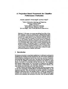
Fig. 1: Profile-based Goal-Directed Performance Tuning
with a range of appropriate tools, we hope to pave the way for the incorporation of this method within future generation compilers so that it can be fully automated. Such compilers could then afford to incorporate very elaborate tuning techniques since they would be called upon only when and where needed, and applied there only to the necessary degree. 3.1 Hierarchical Optimization Figure 1 illustrates the incremental/dynamic optimization process. First, performance profiling reports raw performance metrics or traces runtime events, which are then analyzed to characterize performance of the target application. Based on this characterization, performance tuning is applied to improve performance by modifying either the application code or the machine. Such an optimization process can be carried out between application runs as needed, i.e. by incremental optimization. The costs of carrying out performance analysis and tuning do not incur runtime overhead. Additionally, dynamic optimization can be employed, but to be effective, the runtime overhead it incurs must be within an acceptable range, which requires both hardware performance monitoring support and the use of only a limited range of optimization techniques. Numerous performance problems can be solved with static compiler techniques, which incur no runtime overhead. Compilers can thus employ a broad range of analyses and optimizations for static optimization. Unfortunately, some elaborate compiler optimizations can be extremely time-consuming, and they are often not considered for commercial compilers. Furthermore, tasks such as performance modeling, interprocedural analysis, and disambiguation of indirect data references, are very timeconsuming or even impossible for a compiler to perform. In our opinion, they can be better addressed by profiling and using a profile-driven incremental/dynamic
increased cost actual execution
machine configuration input profile
code Application Information
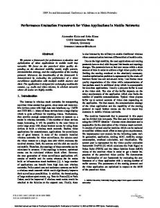
dynamic optimization just-in-time optimization incremental optimization static optimization Optimization
Fig. 2: A Hierarchical View of the Information Used by the Four Optimization Schemes
approach. More elaborate optimization techniques then become attractive as they can be employed selectively only when they will be most effective as determined by adequate profiling and analysis. The above discussion is illustrated in Figure 2, which compares the general cost (the overhead and the software/hardware support) and coverage (the range of targeted problems) of the four different optimization schemes (levels) and shows the sources of application information that are available to each of them. Generally, the closer to the actual execution, the more information can be made available, but the cost of optimization rises as it demands more hardware/software support and the time required to carry out optimization becomes more critical. Thus, fewer problems can be solved in the affordable time as the execution time approaches. Therefore, while it seems logical to delay solving performance problems until further information is gathered, it is best to solve particular types of problems as early as possible. The recommended hierarchical approach toward optimizing an application is to: (1) apply static optimization first, (2) address unsolved, semi-dynamic performance problems (problems that become tractable with profiling or tracing) with incremental optimization, (3) perform input- or machine-specific optimization with JIT compilation, and (4) use dynamic optimization to detect and solve problems that occur dynamically at runtime. The techniques discussed in Section 3.2 and Section 3.3 are designed to address these issues in this manner.
3.2 Goal-Directed Compilation For optimizing the performance of an application, the goal is to minimize the overall application runtime. Reducing the overhead caused by multiple problems does not necessarily amount to eliminating individual problems. Furthermore, optimizing overall application performance is more difficult than optimizing the performance of individual routines locally. For the purpose of successfully directing the compilation process toward the goal, we need a method for gauging the distance to the goal and distinguishing the significance of each individual problem. In this subsection, we discuss the use of hierarchical performance bounds to realize such a goal-directed compilation. 3.2.1 Hierarchical Performance Bounds A performance bound is an upper bound on the best achievable performance. For assessing the performance of an entire application, performance is best measured by the total runtime, rather than by bandwidth or rate-based metrics such as MFLOPS. Hierarchical machine-application bounds models, collectively called the MACS bounds hierarchy, have been used to characterize application performance by exposing performance gaps between the successive levels of the hierarchy [1][3][4]. The MACS machine-application performance bound methodology provides a series of upper bounds on the best achievable performance (equivalently, lower bounds on the runtime) and has been used for a variety of loop-dominated applications on vector, superscalar and other architectures. The hierarchy of bounds equations is based on the peak performance of a Machine of interest (M), considering also a high level Application code of interest (MA), the Compiler-generated workload (MAC), and the actual compiler-generated Schedule for this workload (MACS), respectively. The MACS bounds hierarchy is extended here to characterize application performance on parallel computers. The extended hierarchy addresses cache misses in the shared-memory system and the runtime overhead due to degree of parallelization, load imbalance, multiple program regions with different workload distributions, dynamic load imbalance, and I/O and operating system interference. This performance bounds hierarchy [5], as shown in Figure 3, successively includes major constraints that often limit the delivered performance of parallel applications. Beyond the MACS bounds, additional constraints are included in the order of: finite cache effect (MACS$ or I bound), partial application parallelization (IP bound), communication overhead (IPC bound), I/O and operating system interference (IPCO bound), overall 1 load imbalance (IPCOL bound), multiple phase load imbalance (IPCOLM bound), and dynamic load imbalance (IPCOLMD bound). We have found this ordering to be
1. Overall load imbalance refers to the imbalance in the distribution of the total load assigned to each processor over the entire application.
System Constraints
Gaps
Execution Time Actual runtime
Unmodeled effects
X
Dynamic load imbalance
D
Parallel Bou nds
IPCOLM-Dynamic (IPCOLMD) bound IPCOL-Multiphase (IPCOLM) bound Multiphase load imbalance
M′
Overall load imbalance
L
IPCO-Load imbalance (IPCOL) bound IPC-Operating system (IPCO) bound I/O, Operating System Events
O
Interprocessor communication
C′
IP-Communication (IPC) bound
Uniprocessor Bounds
I-Partial parallelization (IP) bound Partial parallelization
P
Finite cache effect
$
Data dependency, branches, pipeline bubbles
S
Compiler-inserted operations
C
Ideal-parallelization (I) bound MACS-Cache (MACS$) bound MAC-Schedule (MACS) bound MA-Compiler (MAC) bound M-Application (MA) bound
Mismatched application workload
A Machine (M) bound
Machine peak performance
M
Fig. 3: Performance Constraints and the Performance Bounds Hierarchy.
intuitive and useful in aiding the performance tuning effort; however, other variations or refinements could be considered based on application characteristics. Our bounds generation tool, CXbound, calculates the above performance bounds, except IPCOLMD bound, for applications run on HP/Convex SPP-1600, based on profiles generated by CXpa [14]. The gap between two successive bounds is named after the performance constraint that differentiates the two bounds. However, while we tried to assign a different letter to each new gap, the letters C and M are each repeated twice in the bounds hierarchy. To avoid confusion, we shall refer to the Communication gap and Multiphase gap as C′ gap and M′ gap, respectively, to distinguish them from the Compiler inserted instructions gap and the Machine peak performance. The definition and calculation of the bounds hierarchy is presented below. The use of the bounds hierarchy for goal-directed optimization is discussed in Section 3.2.2.
Machine Peak Performance: M Bound The Machine (M) bound is defined as the minimum run time if the application workload were executed at the peak rate. The minimum workload required by the application is indicated by the total number of operations1 observed in the high-level source code of the application. The machine peak performance is specified by the maximum number of operations that can be executed by the machine per second. The M bound (in seconds) can be computed by M Bound = (Total Number of Operations in Source Code)/ (Machine Peak Performance in Operations per Second).
Application Workload: MA Bound The MA bound considers the fact that an application has various types of operations that have different execution times and use different processor resources (functional units). Functional units are selected for evaluation if they are deemed likely to be a performance bottleneck in some common situations. The MA bound of an application counts the operations for each selected function unit from the high level code of the application, the utilization of each functional unit is calculated, and the MA bound is determined by the execution time of the most heavily utilized functional unit. The MA bound thus assumes that no data or control dependencies exist in the code and that any operation can be scheduled at any time during the execution, so that the function unit(s) with heaviest workload is fully utilized. Compilation: MAC Bound The MAC bound is similar to MA, except that it is computed using the actual operations produced by the compiler, rather than only the operations counted from the high level code. Thus MAC still assumes an ideal schedule, but does account for redundant and unnecessary operations inserted by the compiler as well as those that are necessary in order to orchestrate the code for the machine being evaluated. MAC thus adds one more constraint to the model by using an actual rather than an idealized workload. Instruction Scheduling: MACS Bound The MACS bound, in addition to using the actual workload, adds another constraint by using the actual schedule rather than an ideal schedule. The data and control dependencies limit the number of valid instruction schedules and may result in pipeline stalls (bubbles) in the functional units. A valid instruction schedule can require more time to execute than the idealized schedules we assumed in the M, MA, and MAC bounds. 1. In our work on scientific applications, “operations” is taken to mean floating-point operations.
Acquiring the I (MACS$) Bound The I (MACS$) bound measures the minimum run time required to execute the application under an ideal (zero communication overhead and perfectly load balanced) parallel environment with no I/O or OS interference. The I bound for an SPMD application is the average MACS$ bound among the processors. Thus, given the number of processors involved in the execution, N, and the MACS$ bounds on the runtime for individual processors, Ω1, Ω2,..., ΩN, the averaged I bound is calculated as: I Bound = (Σi=1..N Ωi )/N. Acquiring the IP Bound The degree of parallelization in the application is a factor that can limit the parallelism in a parallel execution. The application may contain sequential regions that are executed sequentially by one processor. Let the total computation time in the sequential regions be Ωs and total computation time in the parallel regions be Ω p, the IP bound for an N-processor execution is defined as the minimum time required to execute the application under the assumption that the parallel regions are executed under an ideal parallel environment, i.e. IP Bound = Ωs+Ω p/N, which is also known as Amdahl’s Law. Acquiring the IPC Bound The IPC bound is defined by the minimum time required to execute the application workload with actual communications on actual target processors, under the assumption that the workload in the parallel portions is always perfectly balanced. Note that communications may add extra workload to both the sequential portions and the parallel portions of the application. Amdahl’s Law is reapplied to the increased sequential and parallel workload to acquire the IPC bound for a N-processor execution, i.e. IPC Bound = Ω s′ + Ωp′ /N, where Ω s′ and Ωp′ denote the sequential and parallel workload assumed in the IPC bound. CXbound uses the CPU time in N-processor profiles generated by CXpa to measure the run time that processors spend on computation and communication. The parallel CPU time (Ω p′) that the processors spend in the parallel regions, is calculated by Ω p′ = Σ q Σr cr,q , where cr,q is the total CPU time that processor q spends in parallel region r. The sequential CPU time (Ω s′) is summed over the serial regions.
Acquiring the IPCO Bound In many high-performance applications, input and output for a program occur mostly in the form of accessing mass storage and other peripheral devices (e.g. terminal, network, printer,...etc.). I/O events are mostly handled by the operating system (OS) on modern machines. The OS also handles many other operations, such as virtual memory management and multitasking, in the background. These background OS activities may or may not be originated by the target application, but can greatly affect the performance of the target application. To acquire the IPCO bound for an N-processor execution, CXbound first calculates the sequential execution time (Ωs′′) and parallel execution time (Ωp′′) under the environment that the IPCO bound models: Ω s′′ = Σ q=1..N Σr∈S wr,q , Ωp′′ = Σ q=1..N Σr∈P wr,q , where wr,q is the wall clock time that processor q spent in region r, S is the set of sequential regions, and P is the set of parallel regions. As the wall clock time reported by CXpa, additionally includes the time spent in OS routines, which is not included in the reported CPU time. Then, Amdahl’s Law is reapplied to the increased sequential and parallel execution times under the environment that the IPCO bound models, i.e. IPCO Bound = Ω s′′ + Ω p′′ /N. Acquiring the IPCOL Bound Load imbalance affects the degree of parallelism in the parallel execution. The execution time of an application with load imbalance is bounded by the time required to execute on the most heavily loaded processor. The IPCOL bound is defined as the minimum time required to execute the largest load assigned to one processor, under the assumption that the load from different parallel regions and iterations that is assigned to a particular processor can simply be combined. The total wall clock time that processor q spent in parallel regions is calculated by summing processor q’s wall clock time over the parallel regions, i.e. Ω p,q′′ = Σr∈P wr,q . The IPCOL bound for the parallel regions is determined by the heaviest parallel workload among the processors; the IPCOL bound for the sequential region is carried over from the IPCO bound (Ωs′′). Τhe IPCOL bound is thus IPCOL Bound = Ωs′′+ Max q=1..N {Ω p,q′′}. In Figure 4, we illustrate how the IPCO and IPCOL bounds are calculated from a performance profile. The example run consists of a two-iteration loop, in which two parallel regions are each executed on two processors. Figure 4(a) shows the workload
distribution for this example. Since this example contains no sequential region, the IPCO bound (41) is essentially the average workload over the two processors, and the IPCOL bound (42) is the maximum overall workload between the two processors, as calculated in Figure 4(b). As indicated by the L gap, the load imbalance of overall workload causes an overhead of 1, which amounts to a 2.43% increase in execution time over a perfectly balanced execution. Acquiring the IPCOLM Bound The IPCOLM bound characterizes the multiphase load imbalance in the application. Multiphase load imbalance usually results from different workload distributions in different program phases of the application that are separated by barrier synchronizations. The execution time for each parallel region is determined by the most heavily loaded processor (the longest running thread) in that region. The IPCOLM bound is calculated by summing the execution time of the longest thread over the individual program regions, namely IPCOLM Bound = Ω s′′ + Σ r∈P Max q=1..N {wr,q}. where wr,q , Ω s′′, and N are as above. The Multiphase (M′) gap (IPCOLM - IPCOL) characterizes the performance impact of multiphase load imbalance. Note that an application can pose serious multiphase load imbalance and still be well balanced in terms of total workload. As we illustrate in Figure 4(c), the calculation of the IPCOLM bound finds the local maxima for individual parallel regions and hence is never smaller than the IPCOL bound. The multiphase load imbalance in this example causes an M’ gap of 4, which equals 4/42 = 9.5% runtime increase over the IPCOL bound. Actual Run Time and Dynamic Behavior The actual run time is measured by the wall clock time of the entire application. The gap between the actual run time and the IPCOLM bound (unmodeled gap) should characterize both dynamic behavior and other factors that have not been modeled in the IPCOLM bound, e.g. the cost of spawn/join and synchronization operations. Dynamic workload behavior can occur if the problem domain or the workload distribution over the domain changes over time. This happens often in programs that model dynamic systems. Dynamic behavior can result in an unpredictable load distribution and renders static load balancing techniques ineffective. An IPCOLMD bound could be generated, as in Figure 4(d), to model the dynamic workload behavior if the execution time for each individual iteration is separately reported, i.e. IPCOLMD Bound = Ωs′′ + Σ r∈P Σ i=1,Num_Iter Max q=1,N {wr,q,i } . where wr,q,i is the wall clock time that processor q spent in region r for iteration i, and Num_Iter is the number of iterations.
Iter./Region
Load on Proc 0
Load on Proc 1
1/1
10
5
1/2
10
15
2/1
5
6
2/2
15
16
(a) A Profile Example. Iter./Regions
Load on Proc 0
Load on Proc 1
All/All
40
42
IPCO Bound = (40 + 42)/2 = 41 IPCOL Bound = Max{40, 42} = 42 Load Imbalance Gap = IPCOL - IPCO = 42 - 41 = 1 (b) Calculation of the IPCO and IPCOL Bounds. Iter./Region
Load on Proc 0
Load on Proc 1
Max. Load
All/1
15
11
15
All/2
25
31
31
IPCOLM Bound = (Max. Load of Phase 1) + (Max. Load of Phase 2) = 15+31 = 46 Multiphase Gap = IPCOLM - IPCOL = 46 - 42 = 4 (c) Calculation of the IPCOLM Bound. Iter./Region
Load on Proc 0
Load on Proc 1
Max. Load
1/1
10
5
10
1/2
10
15
15
2/1
5
6
6
2/2
15
16
16
IPCOLMD Bound =
Σ(Max. Load in each region for each iteration)
=
10+15+6+16 = 47
Dynamic Gap = IPCOLMD - IPCOLM = 47 - 46 = 1 (d) Calculation of the IPCOLMD Bound. Fig. 4: Calculation of the IPCO, IPCOL, IPCOLM, IPCOLMD Bounds.
Iteration/Region
Load on Proc 0
Load on Proc 1
1/1
15
5
1/2
5
15
2/1
5
15
2/2
15
5
(a) A Profile Example Bound
Value
Gap from Previous Bound
IPCO
40
N/A
IPCOL
40
0
IPCOLM
40
0
IPCOLMD
60
20
(b) Calculation of the IPCO and IPCOL Bounds Fig. 5: An Example with Dynamic Load Imbalance.
The Dynamic (D) gap characterizes the performance impact of the dynamic load imbalance in the application. The D gap in the above example is primarily due to the change of load distribution in region 1 from iteration 1 to iteration 2. A more dynamic example is given in Figure 5(a), and the performance problem, i.e. the dynamic behavior, is revealed via the bounds analysis shown in Figure 5(b). A severe D gap, for example, may be reduced by relaxing the synchronization between iterations or finding a better static domain decomposition, or may require dynamic decomposition. Unfortunately, CXpa is not suitable for measuring the execution time for each individual iteration, and hence CXbound cannot generate the IPCOLMD bound. So far, we have not found a proper tool to solve this problem on the HP/Convex Exemplar. Thus, in the case studies of Section 4, the dynamic behavior effects are lumped together with the other “unmodeled effects” as the unmodeled (X) gap which is then calculated as (Actual Execution Time) - (IPCOLM Bound). 3.2.2 Goal-Directed Optimization In ascending through the bounds hierarchy from the M bound, the model becomes increasingly constrained as it moves in several steps from potentially deliverable toward actually delivered performance. Each gap between successive performance bounds exposes and quantifies the performance impact of specific runtime constraints, and collectively these gaps identify the bottlenecks in application performance. Performance tuning actions with the greatest potential performance gains can be selected according to which gaps are the largest, and their underlying causes. This approach is referred to as goal-directed performance tuning or goal-directed compila-
Serial Program
Step 1 Partition the Problem Domain
C’, L, M’, D-gap
Step 2
Step 4
Step 6
Tune Communication Performance
Balance Load for Single Phases
C’-gap
L-gap
Balance Combined Load for Multiple Phases
Step 7 Balance Dynamic Load
M’-gap
D-gap
Step 3 Optimize Processor Performance
A, C, S, $-gap
Step 5 Reduce Synchronization Overhead
L, M’ ,D-gap
Performance-tuned Parallel Program Fig. 6: Performance Tuning Steps and Performance Gaps.
tion [5][4], which can be used to assist hand-tuning, or implemented within a goaldirected compiler for general use. We utilize the hierarchical bounds model in implementing a goal-directed optimization strategy. As illustrated in Figure 6, we associate specific performance gaps with several key performance tuning steps in our application tuning work. Before each step, we consider specific gap(s). For example, the actions in Step 1 (partitioning) are associated with gaps C’, L, M’, and D. Significant gaps help guide what specific performance tuning actions should be considered for each step. A step may be skipped if there is no significant gap associated with that step. After one or more performance tuning actions are applied, the bounds hierarchy can be re-calculated to evaluate the effectiveness and the side-effects of these actions.
The numbers show the order of the steps, and the arrows show the dependence between the steps. When the program is modified in a certain step, the earlier steps found by following the backward arrows may need to be performed again as they may conflict with or be able to take advantage of the modification. For example, load balancing techniques in Steps 4, 6 and 7 may suggest different partitionings of the domain, which would cause different communication patterns that may need to be reoptimized in Step 2. Changing the memory layout of arrays to eliminate false sharing in Step 2 might conflict with certain data layout techniques that improve processor performance in Step 3. Changing communication and processor performance may affect the load distribution which then needs to be re-balanced. In general, this graph detects various types of performance problems in an ordered sequence, and a step needs to be repeated only if particular problems are detected that need to be dealt with. Less aggressive optimization techniques that are more compatible with one another are better choices in the earlier phases of code development. For each step, we identify the relevant performance issues and possible actions to address them. Table 1 [5] shows such a grouping. For example, tuning action (AC29), Self-Scheduling, may be selected to solve issue (I-15), Balancing a Nonuniformly Distributed Load, for targeting the L gap gauged by the hierarchical performance analysis, but it can affect other issues either positively (for issues 16, 18, 19, and 20) or negatively (for issues 2 and 17). The “Other Affected Issues” column lists the issues are deemed likely to be affected, either positively or negatively. The gaps associated with the affected issues are also likely to change, and thus should be examined for evaluating the applied action and choosing the next action. This table categorizes the performance issues and gaps that would be affected by each tuning action, and thus provides a mechanism for evaluating tuning actions with hierarchical performance bounds in an incremental optimization process. The tuning actions listed above should be viewed as the beginning of an open extensible set. Systems should provide performance monitoring metrics that are sufficient for evaluating the bounds, so as to identify the performance issues that are most critical to address. The list of possible tuning actions should include all optimizations that the available compilers, precompilation tools, and run-time environments might perform (and others that may involve programmer assistance), except for those routine or local optimizations that conventional optimizers already perform well on their own without the goal-directed assistance of this framework. With this framework, a large set of aggressive optimization techniques can be included. Such techniques are often not implemented in commercial optimizers today due to the high overhead of performing the optimization and the weak, overgeneralized, and heuristic state of the art that chooses when, where and how to apply them. However, this framework carefully selects these optimizations only when necessary and employs them to the extent necessary, precisely where they are deemed to be most beneficial. It thus enhances the benefits, and reduces the overhead and risks of incorporating aggressive optimizations.
Tuning Step
Performance Issue
Partition (I-1) Partitionthe Problem ing an Irregu(Step 1) lar Domain
Tuning Actions
(A-1) Applying a Proper Domain Decomposition Algorithm for (I-1)
Targeted Primarily Positive Negative Other Perform- Affected for for Affected ance PerformIssues Issues Issues Gap(s) in ance this Step Gap(s) (1)
-
(3)(6)(15) (18)(19)
P
$, P, C’, L, M’, D
(2)
-
(4)(5)(12) (14)
C’
$, C’
(2)
-
(1)(4)(12) (15)(18) (19)
C’
C’, L, M’, D
(3)
-
(1)(6)(15) (18)(19)
C’
C’, L
(4)
-
(5)(12)
C’
C’, $
(4)(5)
(12)
(2)(14)
C’
C’, $, M
(5)
-
(2)(4)(12)
C’
C’, $
(5)
-
(2)(4)(12)
C’
C’, $
(5)
-
(2)(4)(12)
C’
C’, $
(5)
-
(4)(7)(9)
C’
C’, $
(6)
-
(1)(2)(3) (15)(18) (19)
C’
C’, $, L
(6)
-
(15)(16) (18)(19) (20)
C’
C’
(A-13) Prefetch, Update, and Out-of-order Execution for (I-7)
(7)
-
(12)(14)
C’
C’, $, M
(I-7) Hiding the (A-14) Asynchronous ComCommunication munication via Messages for Latency (I-7)
(7)
-
(4)(5)(9) (14)
C’
C’, $
-
(9)(12)(1 4)
C’
C’, $, S
(8)
(9)
(14)
C’
C’, S
(A-2) Proper Utilization of (I-2) Exploiting Distributed Caches for (I-2) Processor (A-3) Minimizing SubdoLocality main Migration for (I-2) (I-3) Minimizing Interprocessor (A-4) Minimizing the Weight of Cut Edges in Domain Data DepenDecomposition for (I-3) dence (I-4) Reducing (A-5) Array Grouping for (ISuperfluity 4) (A-6) Privatizing Local Data Accesses for (I-5) (A-7) Optimizing the Cache Coherence Protocol for (I-5) (I-5) Reducing Unnecessary (A-8) Cache-Control DirecCoherence tives for (I-5) Operations (A-9) Relaxed Consistency Memory Models for (I-5) (A-10) Message-Passing Directives for (I-5) Tuning the (A-11) Hierarchical PartiCommunitioning for (I-6) cation Per- (I-6) Reducing formance the Communica(A-12) Optimizing the Sub(Step 2) tion Distance domain-Processor Mapping for (I-6)
(A-15) Multithreading for (I(7)(13) 7) (I-8) Reducing (A-16) Grouping Messages for (I-8) the Number of Communication (A-17) Using Long-Block Transactions Memory Access for (I-8)
(8)
(4)(5)(9)
(14)
C’
C’, S, $
(I-9) Distributing the Commu- (A-18) Selective Communinications in cation for (I-9) Space
(8)
-
(14)
C’
C’
(I-10) Distributing the Commu- (A-19) Overdecomposition to Scramble the Execution nications in for (I-10) Time
(9)
-
(14)
C’
C’, S, $
Table 1: Performance Tuning Steps, Issues, Actions and the Effects of Actions (1 of 3).
Tuning Step
Performance Issue
Tuning Actions
(A-20) Properly Using Compilers or Compiler Directives for (I-11) Choosing (I-11) a Compiler or Compiler Direc- (A-21) Goal-Directed Tuntive ing for Processor Performance for (I-11)
(11)
-
-
C, S, $
C, S, $, C’
(11)
-
-
-
-
(12)
(2)
(4)(14)
$
$, C
(12)
(2)
(4)(14)
$
$, C
(12)
-
(14)
$
$, C
(13)
-
(7)
$
$, C, M, S
(13)
-
(7)
$
$, C, S
(A-27) Repeating Steps 2 and 3 for (I-14)
(14)
-
(A-28) Profile-Driven Domain Decomposition for (I-15)
(15)
(A-29) Self-Scheduling for (I-15)
(15)(16) (18)(19) (20)
(A-22) Cache Control Directives for (I-12) (I-12) Reducing (A-23) Enhancing Spatial Locality by Array Grouping the Cache for (I-12) Capacity Misses Optimizing (A-24) Blocking Loops Processor Using Overdecomposition Perforfor (I-12) mance (A-25) Hiding Cache Miss (Step 3) Latency with Prefetch and (I-13) Reducing Out-of-Order Execution for (I-13) the Impact of Cache Misses (A-26) Hiding Memory Access Latency with Multithreading for (I-13) (I-14) Reducing Conflicts of Interest between Improving Processor Performance and Communication Performance Balancing the Load per Phase (Step 4)
(I-15) Balancing a Nonuniformly Distributed Load
Targeted Primarily Positive Negative Other Perform- Affected for for Affected ance PerformIssues Issues Issues Gap(s) in ance this Step Gap(s)
(2)-(13) C, S, $, C’ C, S, $, C’
(1)(3) (18)(19) (2)(17)
L
L, C’
L
L, C’, M’, D
Table 1: Performance Tuning Steps, Issues, Actions and the Effects of Actions (2 of 3).
3.3 Model-Driven Performance Tuning Figure 7 shows a framework, called Model-Driven Performance Tuning (MDPT) that can be used to accelerate the performance analysis and tuning process by exploiting the use of an application model (AM), a parsed form (intermediate representation) of the application code generated and used within compilation. The AM is annotated with profile information, an abstraction of the application behavior derived from performance assessment, as shown in Figure 8. Driven by this application model and a machine model (a machine performance characterization created from specifications and microbenchmarking), Model-Driven Simulation (MDS), analyzes and projects
Tuning Step
Performance Issue
Tuning Actions
Targeted Primarily Positive Negative Other Perform- Affected for for Affected ance PerformIssues Issues Issues Gap(s) in ance this Step Gap(s)
(A-30) Fuzzy Barriers for (I- (16)(18) 16) (19)(20) (I-16) Reducing (A-31) Point-to-Point SynReducing the Impact of chronizations for (I-16) the Syn- Load Imbalance (A-32) Self-scheduling of chronizaOverdecomposed Subdotion/ mains for (I-16) Scheduling Overhead (I-17) Reducing (Step 5) the Overall Scheduling/Synchronization Overhead
-
(17)
L, M’
L, M’, D
(16)(18) (19)(20)
-
(17)
L, M’
L, M’, D
(2)(16)
-
(16)(17) (18)(19)
L, M’
L, M’, D
-
-
-
L, M’, D
L, C’, M’, D
(18)
(3)(15)
M’
M’, L, D
(A-33) Balancing the Most Critical Phase for (I-18) Balancing the Com(I-18) Balancbined Load ing the Load for for Multia Multiphase ple Phases Program (Step 6)
(A-34) Multiple Domain Decompositions for (I-18)
(18)
-
(3)
M’
M’, C’, L, D
(A-35) Multiple-Weight Domain Decomposition Algorithms for (I-18)
(2)(18)
-
(3)(15)(1 9)
M’
M’, L, D
(A-36) Fusing the Phases and Balancing the Total Load for (I-18)
(16)(18)
-
(15)(20)
M’
M’, L, D
(2)
(3)(14)
D
D, C’, L, M’
(2)
(3)(15) (17)(18)
D
D, C’, L, M’
-
(3)(15)(1 9)
D
D, C’, L, M’
-
(14)(17)( 18)
D
D, C’, L, M’
(A-37) Dynamically Redecomposing the Domain for (19)(20) (I-19) (I-19) Reducing the Dynamic (A-38) Dynamic/Self-Sched- (16)(19) uling for (I-19) (20) Balancing Load Imbalance Dynamic (A-39) Multiple-Weight Load Domain Decomposition for (2)(19) (Step 7) (I-19) (I-20) Tolerating the Impact (A-40) Relaxed Synchroniza(16)(19) of Dynamic tions for (I-20) Load Imbalance
Table 1: Performance Tuning Steps, Issues, Actions and the Effects of Actions (3 of 3).
the application performance by simulating the machine-application interactions on the model and issuing reports, as shown in Figure 9. In MDPT, the application model, instead of the application, becomes the object of performance tuning. Proposed performance tuning actions are first installed in the application model and evaluated via MDS to assist the user in making tuning decisions. This concept of the MDPT approach, the capabilities it provides, and its potential are discussed below (each numbered paragraph is keyed to the corresponding number in Figure 7): 1. Various sources of performance assessment and program analysis contribute to the application modeling phase for providing a more complete, accurate model. Performance assessment tools and application developers both contribute to creating the application model.
modifying the application code (6) application performance profiling
application model (AM)
modifying the application model
(3)
(1) (2)
application developer
machine characterization
performance tuning
model-driven simulation (MDS)
(4)
machine model
(5) adjusting the machine model
machine adjusting the machine (6)
Fig. 7: Model-Driven Performance Tuning.
2. In the performance modeling phase, MDS is carried out to derive information by analyzing the machine-application interactions between the application model and the machine model. The machine model is based on the machine specification and/or the results of machine characterization. 3. The application model serves as a medium for experimenting with the application of performance tuning techniques as well as resolving the conflicts among them. In MDPT, performance tuning techniques are first iteratively applied and evaluated on the application model using MDS (see cycle (3)) and only ported to the code (via cycle (6)) after reaching a desirable plateau. Such use of this short loop for what-if evaluations should significantly shorten the overall application development time. 4. The application model can be tuned by either the programmer or the compiler. A properly abstracted application model helps the user or the compiler assess the application performance at an adequate level, without the overkill burden of tuning by carrying out transformations and performance analysis directly on the application and repeatedly handling the high volume of raw performance data that is produced. Performance tuning uses the output reports of MDS (Figure 9) to select tuning actions from Table . 5. In addition to tuning the application model, the machine model can be tuned to improve the application performance. Using MDS, the users are given the opportunity to evaluate various machine configurations or different machines for specific applications without actually reconfiguring or building the machine. 6. After tuning actions are evaluated with MDS and accepted, they are applied to the application code and/or the target machine to assess the actual improvement, validate, and possibly recalibrate the models.
machine
program
input data
Application
profile-driven analysis
trace-driven analysis
source-code analysis
domain decomposition algorithm
Analysis
weight distribution
control flow
data dependence
domain decomposition
layout
Application Model Fig. 8: Building an Application Model.
3.3.1 Application Modeling The Application Modeling (AM) phase generates specifications of the application behavior, including the application’s control flow, data dependence, domain decomposition, and the weight distribution over the domain. This phase can be carried out by the application developer with minimal knowledge about machine-application interactions. We have designed a language, called the Application Modeling Language (AML) for the user to specify the application model and incorporate results from performance assessment tools, such as profiling. The performance of an application is fundamentally governed by (1) the program (algorithm), (2) the input (data domain/structures), and (3) the machine that are used to execute the application. It is relatively difficult to observe machine-application interactions at this level, since detailed machine operations are often hidden from the programming model that is available to the programmer. We would like to model the application at a level that provides us with more precise information on how the application behaves, especially the behavior that directly affects performance. The control flow and the data dependence in the application are modeled because they limit the instruction schedule and determine the data access pattern for the application. The decomposition of the input data determines the decomposition of the workload (for an SPMD application). The layout of the data structure determines the data allocation and affects the actual data flow in the machine, especially for a cache-based, distributed shared-memory application. The
workload in the application certainly requires resources from the processors and hence needs to be modeled for addressing load balance problems. An application model is acquired by abstracting (1) control flow, (2) data dependence, (3) domain decomposition, (4) data layout, and (5) the weight distribution (workload) from the application. These five components are hereafter referred to as modules of the application model. Figure 8 illustrates how we model applications on the HP/Convex SPP-1600 via the use of source code analysis (mostly done by the programmer), profiling (CXpa), and trace-driven simulation tools (Smait and CIAT/CCAT [15]). In this flow chart, a solid line indicates a path that we currently employ to create a particular module, and a dashed line indicates an additional path that might be useful for creating the module. We briefly describe the process used to create these modules as follows: • The control structure, the data dependence, and the data layout that are encoded in the program are abstracted via source code analysis. While analyzing irregular applications can be difficult for compilers, this task can be eased with profiling and tracing, and programmer assistance where needed. However, since compilers are useful for analyzing most regular applications without assistance, we assume that the generation of these modules can be done mostly by converting the results of compiler analysis (from the internal representation used by the compiler). • We use weights to represent the application workload in different code sections. Although the instruction sequence in a code section can be extracted to model the workload, accurately predicting the execution time of the code section based on the instruction sequence can be rather complicated and difficult. Profile-driven analysis can be used straightforwardly by the user for extracting the weights where the load is uniformly-distributed. For non-uniformly-distributed cases, techniques such as the weight classification and predication method [18] may be needed. • In an SPMD application, the computation is decomposed by decomposing the domain. The domain decomposition can be implicitly specified in the application by DOALL statements, or explicitly programmed into the code according to the output of a domain decomposition package such as Metis [17]. The data dependence and the weight distribution of the application are given as inputs to the domain decomposition package. We believe that building such an application model is highly feasible for the application developers with the programming tools available today. Most of the above procedures involved in modeling an application require very little knowledge about the target machine, and tools such as profiling provide additional help in measuring the workload and in helping the programmer to extract the application behavior. 3.3.2 Model-Driven Performance Evaluation The Model-Driven Simulation (MDS) derives performance information based on the application model by analyzing the data flow, working set, cache utilization, workload, degree of parallelism, communication pattern, and the hierarchical performance bounds. MDS performs a broad range of analyses that use combinations of conven-
Machine & Application Models machine model
weight distribution
control flow
workload analysis
domain decomposition
data dependence
layout
working set & data flow analysis
communication analysis
cache analysis
CXbound analysis MDS Performance Bounds Timing Load Imbalance Synchronization Cost Scheduling Cost
Data Flow
Cache Misses
Communication Pattern
Fig. 9: Model-driven Analyses Performed in MDS.
tional performance assessment tools. Results from MDS are used to validate the application model by comparing results with those of previous performance assessments in known cases (both cases that were previously used to generate the model, as well as new cases with new profiles). MDS is a performance analyzer that derives performance information for an application by simulating the application’s model with a machine model. MDS is a modeldriven simulator that executes the tasks in the application model as if executing a Fortran or C program. Figure 9 shows the performance analyses that are carried out in MDS. MDS follows the flow defined in the control flow module. When a task is executed, MDS performs the operations required by the task according to the modules associated with the task. MDS handles a task according to the following steps: 1. The domain decomposition module is used to group the iteration space into subdomains. The workload for one sub-domain forms a sub-task.
2. The scheduling policy attribute of the task is used to map each sub-task to one processor, say P i, which is responsible for executing the sub-task. 3. Find the sub-task’s data dependence statement in its data dependence module and mark the data read and/or written in the sub-task. The user can configure MDS to perform the following inherent data analyses: 3a. Working set analysis: MDS calculates the volume of data accessed in the task. 3b.Data flow analysis: MDS records a Read-after-Write (RAW) transaction if the sub-task reads a data item which was a written by a previous sub-task. 4. The user can configure MDS to analyze the data accesses with memory addresses generated using the (sub)task’s data layout module. Using the addresses, MDS can perform the following functions: 4a. Memory reference trace generation: MDS outputs the addresses and the types of the data references in the task to the trace file associated with Pi. 4b.Coherence communication analysis: a shared-memory simulation is carried out to identify the memory references that would cause interprocessor communications under the infinite-cache assumption. 4c. Communication latency analysis: the communication latency that the (sub)task experiences is estimated based on the distance and type of communications, as characterized in the machine model. 5. The weight distribution module calculates the computational weight for the subtask. 6. The execution time counter for Pi, denoted Texec(Pi ) is updated by adding the computational weight and the communication latency of the (sub)task to the previous T exec(Pi). When a synchronization point is reached, MDS finishes executing all the (sub)tasks that are prior to the synchronization and may selectively execute independent (sub)tasks if a relaxed synchronization is used. At the synchronization point, MDS calculates a few time stamps for the synchronization. MDS reports a profile of the simulated performance by recording the computation time, communication event counts and latency for each task or loop on each processor, as well as the load imbalance for each parallel region. Based on this profile, MDS calculates the parallel hierarchical performance bounds for the application, using the CXbound methodology discussed in Section 3.2.1. Thus far, we have successfully modeled several programs from the NAS Parallel Benchmarks [19] as well as CRASH (Section 4.1). The syntax of the AML application modeling language is quite simple and limited in these preliminary studies; however, even as currently implemented, our model-driven tools were found to be effective in predicting and analyzing application performance as well as in guiding the selection of tuning actions within the goal-directed optimization process.
program CRASH repeat c First phase: generate contact forces do i=1,Num_Elements Force(i)=Contact_force(Pos(i),Vel(i)) do j=1,Num_Neighbors(i) Force(i)=Force(i)+Calculate_force(Pos(i),Vel(i), Pos(Neighbor(j,i),Vel(Neighbor(j,i)) end do end do c
Second phase: update position and velocity do i=1,Num_Elements if (Type(i) .eq. plastic) then call Update_plastic(i, Pos(i), Vel(i), Force(i)) else if (Type(i) .eq. elastic) then call Update_elastic(i, Pos(i), Vel(i), Force(i)) end if end do until (end_condition) end Fig. 10: Pseudo Code of CRASH.
4
Preliminary Case Studies
In this section, we improve the performance of CRASH and FSS-PRISM [20] by applying our goal-directed performance tuning scheme in conjunction with our model-driven performance tuning approach. 4.1 CRASH CRASH is a highly simplified code that realistically represents several problems that arise in an actual vehicle crash simulation. It is used here for demonstrating these problems and their solutions. A simplified high level sketch of the serial version of this code is given in Figure 10. CRASH exhibits irregularity in several aspects: indirect array indexing, unstructured meshes, and nonuniform load distribution. Because of its large data set size, communication overhead, multiple phase and dynamic load balance problems, this application requires extensive performance-tuning to perform efficiently on a parallel computer. CRASH simulates the collision of objects and carries out the simulation cycle by cycle in discrete time. The vehicle is represented by a finite element mesh which is provided as input to the code. Elements in the finite-element mesh are numbered from 1 to Num_Elements. The number of elements varies with the detail level of the vehicle model. The program calculates the forces between elements and updates the status of each element for each cycle. In the first phase, the Contact phase, the force applied to each
element is calculated by calling Contact_force() to obtain and sum the forces between this element and other elements with which it has come into contact. In second phase, the Update phase, the position and velocity of each element are updated using the force generated in the contact phase. Depending on the type of material, the Update phase calls Update_Plastic() or Update_Elastic() for updating the position and velocity as a function of Force(i). Each cycle thus outputs a new finite-element mesh which is used as input to the next cycle. This example program shows several types of irregularities, which pose a challenge to performance optimization. First, objects are represented by unstructured meshes. Second, in the Contact phase, properties of neighbor elements are referenced with indirect array references, e.g. Vel(Neighbor(j,i)), refers to the velocity of the j-th neighbor of element i. Third, the load is nonuniform because the load of calculating the force for an element during the Contact phase depends on how many neighbors each element has, and the load of updating the status of an element during the Update phase depends on the type of element being updated. Below, we apply our goaldirected and model-driven optimization process, and describe the resulting series of tuning actions and their results. 4.1.1 CRASH-SP The parallelism in CRASH can quite easily be recognized by a parallel programmer: the calculations for different elements within each phase can be performed in parallel, because they have no data dependence. Manual parallelization of CRASH can be implemented by parallelizing the major loop in each phase (indexed by i). In a straightforward, simple parallel version, called CRASH-SP, each of the two phases is parallelized by partitioning the index into consecutive sub-domains, i.e. elements {1,2, ... N/p } are assigned to processor 1, elements { N/p+1 ... 2N/p } are assigned to processor 2, etc., where N is Num_Elements and p is the number of processors used in the execution. Since this parallelization partitions the domain into sub-domains of nearly equal size, the workload will be evenly shared among the processors, if the load is evenly distributed over the index domain. However, for irregular applications like CRASH, this simple decomposition could lead to enormous communication traffic and poor load balance due to the unstructured meshes and nonuniform load distribution. The performance bounds analysis for CRASH-SP is shown in Figure 11, which reveals the major performance gaps and their causes: • S’-gap (49.4% of the runtime): synchronization cost for executing the barriers. • Unmodeled (X) gap (17.8% of the runtime): false-sharing communications and other unknown factors. • C’-gap (3.4% of the runtime): communications. • L-gap (3.0% of the runtime): overall load imbalance.
100% 90%
X
80% 70% 60%
Unmodeled S'-gap
S’
M'-gap
50%
L-gap C'-gap
40% L C’
30% 20%
P-gap I-bound
I
10% 0% SP
Fig. 11: Performance Bounds Analysis for CRASH-SP.
4.1.2 CRASH-SD Initially, as stated in Step 1 of our goal-directed approach (see Section 3.2), we would like to improve the domain decomposition in CRASH-SP. We incorporated a domain decomposition scheme in a new version, called CRASH-SD, to reduce the overhead due to communication and load imbalance. As shown in Figure 12, the C’-gap and Lgap in CRASH-SD are, in fact, reduced. However, the unmodeled gap is increased due to increased false-sharing communications, whose effects are not modeled by MDS. 4.1.3 CRASH-SD2 Since the expanded unmodeled gap caused by the false-sharing communications in CRASH-SD are significant, we chose to reduce the communication overhead as our next performance tuning step. To eliminate false-sharing, we use padding to adjust the size of array Pos, Vel, and Force. In CRASH-SD, each of these arrays is defined as a one-dimensional array of vectors, where each vector consists of three 8-byte real numbers. Therefore, each is in fact a two-dimensional array declared as (3,Max_Elements). In CRASH-SD2 we eliminate false-sharing by increasing the size of these arrays to (4,Max_Elements) . Consequently, the unmodeled gap, as shown in Figure 12, is reduced on CRASH-SD2 to about the same size as that of CRASH-SP.
3 Unmodeled
2.5 Time (sec.)
X
S'-gap
2
M'-gap
1.5
L-gap
S’
C'-gap
1
P-gap 0.5
I-bound
I
0 SP
SD
SD2
SD3
SD4
Code
Fig. 12: Comparison of the Performance of CRASH-SP, SD, SD2, SD3, and SD4.
The expanded data layout, however, is less efficient in memory usage and has eight superfluous bytes in each cache block, which affects storage space and communication. The C’-gap, is in fact slightly increased due to the expanded data layout. Nevertheless, the overall performance of CRASH-SD2 is better than its predecessors. 4.1.4 CRASH-SD3 Arbitrary thread-processor assignment in entering parallel regions would cause data redistribution during the execution of CRASH-SP and CRASH-SD, which is one aspect of machine-application behavior that MDS does not model. As we suspected that this might be the primary cause of the remaining unmodeled gap, we attempted to minimize sub-domain migration by permanently binding sub-domains to processors in CRASH-SD3. CRASH-SD3 spawns threads before the main simulation loop starts. Since each of these threads is responsible for one sub-domain throughout the main simulation loop, the sub-domain cannot migrate during the execution. Figure 12 shows that the unmodeled gap was in fact eliminated in CRASH-SD3. 4.1.5 CRASH-SD4 Since the L-gap (overall load imbalance) is not significant in CRASH-SD3, we skip Step 4 (Balancing the Load for Single Phases). In CRASH-SD4, we attempt to reduce
3 Unmodeled
2.5
S'-gap
Time (sec.)
X
2
M'-gap L-gap
1.5 S’
C'-gap
1
P-gap 0.5
I-bound
I
SD8
SD7
SD6
SD5
SD3 SD4
Ser SP SD SD2
0
Code
Fig. 13: Comparison of the Performance of All CRASH Versions.
the S’-gap by reducing the number of barriers, because the synchronization time is obviously the most significant remaining performance problem in CRASH-SD3. We notice that some of the synchronization barriers used in the previous versions were placed consecutively by the compiler and hence cause redundant synchronization time. This is typical when DOALL loops or automatic parallelization are used in a code, and most compilers today do not attempt to eliminate redundant barriers. These redundant barriers are removed by replacing consecutive barriers with one barrier. Figure 12 shows that CRASH-SD4 is significantly improved over CRASHSD3 due to reduced synchronization overhead (smaller S’-gap). Approximately 50% of the S’-gap is eliminated as a result of removing redundant barriers. 4.1.6 CRASH-SD5, 6, 7, and 8 As the effect of the remaining S’-gap would be much less for a larger, more realistic input data set, we can end the optimization effort after CRASH-SD4. Nevertheless, further fine-tuning is still possible. In [5] (pp. 205-215), we described some additional actions in our attempt (CRASH-SD5, 6, 7, and 8) to reduce the remaining C’ and S’ gaps. While some of these additional actions can effectively improve the performance, e.g. the use of double buffering in CRASH-SD8 cuts the S’ gap in half, the performance loss caused by the side effects of some actions offsets (in CRASH-SD5 and CRASH-SD6) or even exceeds the anticipated performance gain (in CRASHSD7). The overall results of performance tuning process are summarized in Figure 13.
Code Name
Code Modification
Targeted Gap(s) P
P2i
Initial parallel version
P3x
Change of domain decomposition to reduce load imbalance and communication overhead
P4a
P3x + loop interchange for routine A to reduce cache capacity misses
C’
P4b
P4a + loop interchange for routine B to reduce cache capacity misses
C’
P5a
P4b + change of parallelization of loop C to reduce memory requirement
-
P5b
P5a + change of parallelization of loop D to reduce memory requirement
-
P6a
P5b + privatizing data accesses and buffering communications to improve data access efficiency
C’
M’, C’
Table 2: Performance Optimization of FSS-PRISM.
4.1.7 Summary of the CRASH Case Study In this section, we have used our model-driven simulator (MDS) to illustrate the use of application models in predicting and analyzing the performance of various CRASH versions and to guide the selection of tuning actions that move the code from one version to the next. We have applied a series of goal-directed performance tuning actions to improve the performance of CRASH. The performance analysis reports from MDS, in conjunction with the performance profiles from CXpa, provided valuable guidance and evaluation in this performance tuning process. 4.2 FSS-PRISM FSS-PRISM is a hybrid finite element antenna/array analysis simulation application developed by Volakis et al. at the University of Michigan [20]. Here we show the results of applying our tuning approach to the performance optimization of FSSPRISM on the HP/Convex SPP-1600. Table 2 shows the resulting versions of FSS-PRISM, the modification done for each of them, and the performance gap(s) that they aim to reduce. The performance of these codes are revealed by the CXbound results shown in Figure 14. The CXbound performance analysis shows that communication overhead is the major performance problem in FSS-PRISM. Thus, most of the tuning effort is spent on optimizing the communication performance for the steps resulting in codes P3x, P4a, P4b, and P6a. Note that although these analyses were carried out more quickly by using a small (Dipol) input data set, the memory requirements were predicted to be excessive for larger input data sets. Thus P5a and P5b were optimized for large scale simulations.
Execution on 4 Processors, input=Dipol
Execution Time
300 250 200
M'-gap L-gap
150 100 50 0
C'-gap Computation
P2i P3x P4a P4b P5a P5b P6a Code Version Fig. 14: Performance of the FSS-PRISM Codes.
Although Figure 14 indicates that P5b is slower than P4b, for a larger problem executed on more processors, P5b should perform better than P4b. This special case demonstrates the necessity of input and machine-dependent optimization in a wellparameterized space. Without P6a, P4b is best for small problems, but P5b is predicted to be better for large problems. However, P6a is best overall.
5
System Support for Performance Evaluation and Dynamic Optimization
In light of increasingly complex software, hardware, and distributed environments, future high performance computers should provide more integrated and complete performance evaluation and optimization support via hardware and software enhancements to enable efficient, real-time performance evaluation and dynamic optimization (as suggested in the previous sections) for a broad range of applications. This support includes: • Performance monitor/profiling support: Extensive hardware assistance is required to collect accurate and detailed performance data, without compromising the ability to process the collected data in real time so as to reveal performance problems in a timely fashion that are critical to dynamic optimization. The system should be versatile and capable of being controlled by the compiler and/or runtime software in order to select those events and statistics for profiling that are most related to targeted problems.
• Compilation and runtime software support: While static compilation may grossly optimize applications for predictably typical inputs, dynamic optimization can improve the performance further by reorchestrating applications between successive runs of a similar kind, or (with the assistance of dynamic compilation) during the runtime itself. To implement dynamic optimization, in addition to providing proper performance monitoring/profiling support as mentioned above, the system needs to provide an efficient scheme for deciding how to react to changes of application behavior and runtime environment, and permit certain critical software and hardware components to be adjusted on the fly. • Architectural support: In addition to supporting performance monitoring, future computers should provide much stronger support for interprocessor communications in a parallel environment and select among alternative communication mechanisms as a function of the observed application behavior. Hardware attributes, such as the cache coherence protocol, memory consistency model, cache configuration, and memory organization should similarly be alterable to optimize application performance.
6
Conclusion
To provide better system support for dynamic performance evaluation and optimization, we need to develop and refine effective software and hardware mechanisms and techniques for implementation as an integral part of future high performance systems. We are currently extending our goal-directed and model-driven tuning methodology to create a vehicle for experimentation with automatic/dynamic performance tuning as well as for suggesting readily exploitable enhanced features for future high performance and parallel system architectures. The implementation details of our tools and the further information about our projects can be found in [5] and our web site (http:// www.eecs.umich.edu/PPP/).
7
Acknowledgment
This research was supported in part by the Automotive Research Center (U.S. ArmyTACOM), and National Partnership for Advanced Computational Infrastructure (NSF Grant No. ACI-961920). Parallel computer time was provided by the University of Michigan Center of Parallel Computing which is sponsored in part by NSF grant CDA-92-14296.
References 1.
Eric L. Boyd and Edward S. Davidson. Hierarchical Performance Modeling with MACS: A Case Study of the Convex C-240. Proceedings of the 20th International Symposium on Computer Architecture, pp. 203-212, May 1993.
2.
3.
4.
5.
6. 7. 8. 9. 10. 11. 12.
13. 14. 15. 16.
17.
18. 19. 20.
Karen A. Tomko and Santosh G. Abraham, Data and program restructuring of irregular applications for cache-coherent multiprocessors, In 1994 Proc. International Conference on Supercomputing, pages 214-255, Manchester, England, July 1994. Eric L. Boyd, Waqar Azeem, Hsien-Hsin Lee, Tien-Pao Shih, Shih-Hao Hung, and Edward S. Davidson. A hierarchical approach to modeling and improving the performance of scientific applications on the KSR1. In Proceedings of the 1994 International Conference on Parallel Processing, Vol. III, pp. 188-192, 1994. Tien-Pao Shih. Goal-Directed Performance Tuning for Scientific Applications. Ph.D. Dissertation, Department of Electrical Engineering and Computer Science, The University of Michigan, Ann Arbor, June 1996. Shih-Hao Hung. Optimizing Parallel Applications. Ph.D. Dissertation, Department of Electrical Engineering and Computer Science, University of Michigan, Ann Arbor, June 1998. John L. Hennessy and David A. Patterson. Computer Architecture: A Quantitative Approach, Morgan Kaufmann Publishers, Inc., 1990. Ann H. Hayes, et al. Debugging and Performance Tuning for Parallel Computer Systems. IEEE Computer Society Press, 1996. David E. Culler, Jaswinder P. Singh, and Anoop Gupta. Parallel Computer Architecture. Morgan Kaufmann, 1999. Ian Foster. Design and Building Parallel Programs: Concepts and Tools for Parallel Software Engineering. Addison-Wesley, 1994. Steven S. Muchnick. Advanced Compiler Design and Implementation. Morgan Kaufmann, 1997. Alfred V. Aho, Ravi Sethi, and Jeffrey D. Ullman. Compiler Principles, Techniques and Tools. Addison-Wesley, 1986. Peter L. Deutsch and Allan M. Schiffman. Efficient Implementation of the Smalltalk-80 System, In the 11th ACM SIGACT/SIGPLAN Symp. on Principles of Programming Languages, Salt Lake City, 1984. James Gosling, Bill Joy, and Guy Steele. The Java Language Specification. Addison-Wesley, 1996. Convex Computer Corp., CONVEX CXpa Reference, 2nd Ed., Convex Press,1994. Gheith A. Abandah. Tools for Characterizing Distributed Shared Memory Applications. Technical Report HPL-96-157, HP Laboratories, December 1996. Gheith A. Abandah and Edward S. Davidson. Characterizing shared memory and communication performance: a case study of the Convex SPP-1000, IEEE Transactions on Parallel and Distributed Systems, Vol. 9, No. 2, pp 206-216, Feb 1998. George Karypic and Vipin Kumar. METIS: Unstructured Graph Partitioning and Sparse Matrix Ordering System Version 2.0. Technical Report, The University of Minnesota, 1995. Karen A. Tomko and Edward S. Davidson. Profile driven weighted decomposition. In Proc. 1996 ACM International Conference on Supercomputing, pp. 165-172, May 1996. D. Bailey, et al. The NAS Parallel Benchmarks. Technical Report RNR-94-07, NASA Ames Research Center, March 1994. John Volakis’s Homepage at the University of Michigan. http://www.engin.umich.edu/ ~volakis.