A Framework for the Interleaving of Execution and Planning for Dynamic Tasks by Multiple Agents Eithan Ephrati 1 and Jeffrey S. l~senschein 2 1 Computer Science Department University of Pittsburgh Pittsburgh, PA tantnsh~cs.pitt.edu 2 Institute of Computer Science The Hebrew University Jerusalem, Israel
[email protected] Abstract. The subject of multi-agent planning has been of continuing concern in Distributed Artificial Intelligence (DAI). In this paper, we suggest an approach to the interleaving of execution and planning for dynamic tasks by groups of multiple agents. Agents are dynamically assigned individual tasks that together achieve some dynamically changing global goal. Each agent solves (constructs the plan for) its individual task, then the local plans are merged to determine the next activity step of the entire group in its attempt to accomplish the global goal. Individual tasks may be changed during execution (due to changes in the global goal). The suggested approach reduces overall planning time and derives a plan that approximates the optimal global plan that would have been derived by a central planner. 1
Introduction
The subject of multi-agent planning has been of continuing concern in Distributed Artificial Intelligence (DAI). Some of the earliest work in the field, such as Smith's Contract Net [15] and Corkill's work on distributing the NOAH planner [2], directly addressed the question of how to get groups of agents to carry out coordinated, coherent activity. These questions have occupied researchers both in the Cooperative Problem Solving subarea of DAI (researchers concerned with centrally designed groups of agents with a global goal), as well as those working on Multi-Agent Systems (collections of self-interested agents with no global goal). More recent research on the issue of multi-agent planning includes that of Martial [19, 18], gatz and Rosenschein [10], Durfee [3, 5, 4], and Lansky [12]. The term multi-agent planning has been used to describe both "planning for multiple agents" (where the planning process itself may be centralised), and "planning by multiple agents" (where the planning process is distributed among the agents). In this paper, we are concerned with the latter paradigm:
140
we investigate how a group of agents can cooperatively construct a dynamically changing plan which, as a group, they also carry out. We present a multi-agent planning procedure to achieve a dynamic global goal; that is, the global goal itself may change over time. The procedure relies on the dynamic distribution of individual planning tasks. Agents solve their local tasks, which are then merged into a global plan. By making use of the computational power of multiple agents working in parallel, the process is able to reduce the total elapsed time for planning and is better able to deal with changes in objective as compared to a central planner.
2
The
Scenario
Our scenario involves a group A = { a l , . . . , am} of rn agents. These agents are to achieve at any given time (t) a global goal (G t, which may change over time). Through the distribution of individual planning tasks ( { g l , . . . , gt}) each agent determines p~, the plan (expressed as a set of constraints) that accomplishes its present task(s). Then, based on the individual plans, the agents communicate as they construct the next multiagent step towards the achievement of the global goal. During this interleaved process of planning and execution, some agents m a y be assigned different tasks. For the time being, we assume t h a t the agents are benevolent and cooperative; however, see Section 5. 2.1 -
3
Assumptions and Definitions
The global goal at time t, G t, is a set of predicates, possibly including uninstantiated variables. G t is divided 3 into n tasks [gt, g t , . . . , gtn]" Each task is a set of instantiated (grounded) predicates such that their union satisfies G t (U~g~ ~ Gt). (Tasks are assigned to individual agents only for the purpose of the planning process; the aztuM execution is divided differently.) - Any plan that achieves g~ is denoted by pl. Each such sub-plan is a sequence of operators (opt,..., op t ) that, invoked in the current configuration of the world S t , establishes g~. - Each agent has a cost function (C: OP x A ~ lR) over the domain's operators [8]. The cost of aj's plan cj(pj) is defined to be ~ - - 1 cj(op~).
An
Example
As an example, consider a simple scenario in the slotted blocks world as described in Figure 1. 4 There are two agents (al, a2) and 3 blocks (a,b,c) with a length a Division of tasks is done by a coordinator or a "supervisor" who is in charge of the group of agents. 4 While the blocks world is inappropriate for studying many real-world issues in 9robotics, it remains suitable for the study of abstract goal interactions.
141
of 2 feet each. The ground surface is divided into 30 contiguous marked regions (coordinates) of 1 foot each, aligned in a row. The world may be described by the following relations: Clear(b)--there is no object on b; On(b, x, V/H)--b is located on block x (or at location x) either vertically (V) or horizontally (H); At(x, loc)--the left edge of object x (agent or block) is at loc. The functions r(b) and l(b) return the grid region of b's left edge, and the length of b, respectively. From now on we will use only the first letter of a predicate to denote it.
I,,,
I-T-- 1
I
0
2
4
, I0
12
6
I
I
8
10
i 12
I ~ 14
16
18
20
I
14
I
14
,
,
22
lO
12
16
14
18
16
20
18
20
22.
Fig. 1. A Simple Sticky Blocks World Example The initial state is: { A(at, 0), A(a2, 9), A(a, 12),O(a, 12, H),A(c, 12), O(c, a, H),A(b, 4), O(b, 4, H)}. The available operators (described in a STRIPS-like fashion) are: 5 Takei(b, z, y ) - - take b from x to y (x and y denote either a region or another block).
[cost. IZoc(x) - Zoc(y)l • l(b), p r e c : O(b, x, z), C(b), C(y), A(ai, del: C(y), A(ai, z), A(b, x), a d d : O(b, y, z), A(a,, y), A(b, y)] Move/(al, z, y ) - - G o from x to y.
x), A(b, x)
[cost: Ix - yl, p r e c : A(ai, x), del: A(ai, x), a d d : A(ai, y)] The agent's initial tasks are (respectively): 9o = {A(a, 16), A(b, 16), O(a, b, H)} and 9o = {A(b, 16), A(c, 16), O(b, c, H)}. The combination of these two tasks will eventually establish the global goal G O= {A(a, 16), A(b, 16), O(a, b, g ) } . s The lower part of Figure 1 describes the emergent state of each task if invoked alone. 5 We assume in this specific example that all agents have identical capabilities. The operators are indexed with respect to the agent that performs them. 6 This is reminiscent of Sussman's Anomaly in the single-agent planning scenario-where the plan to achieve one subgoal obstructs the plan that achieves the other [16].
142
After 3 execution time-steps the task gO is change to be {A(a, 16), O(a, c, H)} (-- g~) and gO is cancelled. Given these (changing) tasks, our agents are to go through a planning process that will result in satisfying the final goal.
4
General
Overview
of the Main
Process
In this section, we consider the primary phase of our technique, namely merging the sub-plans that achieve the given task so as to determine the next optimal move of the entire group. A sub-plan is constructed by an agent with only a local view of the overall problem; therefore, conflicts may exist among agents' sub-plans, and redundant actions may also have been generated. Given the set of sub-plans, we are looking for a method to merge them in an optimal (and inexpensive) way. In this section, we describe a cost-driven merging process that results in a coherent global plan (of which the first set of simultaneous operators is most relevant), given the sub-plans. We assume that at each time step t each agent, i, has been assigned (only for the purposes of the planning process) one task. Given that instance, the agent will derive p~, the sub-plan that achieves it. Note that once i has been assigned g~ at any given t, the plan it derives to accomplish it stays valid (for the use of the algorithm) as long as #~ remains the same. That is, for any time t + k such that g~+k = g$, it holds that p~+~ = p~. Therefore, replanning can be modularised among agents; one agent may have to replan, but the others can remain with their previous plans. The process is iterative. The underlying idea is the dynamic generation of alternative execution steps that identifies the optimal global plan and thus the next optimal global execution step. At each step, all agents state additional information about the sub-plan of which they are in charge. The next optimal step is then determined and the current configuration of the world, S t , is changed to be S t+l. The process continues until all tasks have been accomplished (the global goal as of that specific time has been achieved). Plans are represented as sets of absolutely necessary sets of constraints that enable them. Note that when we refer to an individual agent's sub-plan, we are really only concerned with that initial part of the sub-plan that is relevant to the merging process at any specific time step t (which, in turn, might depend on some "look-ahead factor," how many steps of the plan are computed prior to actual execution of a plan step). The way each individual determines this initial part of his sub-plan (i.e., what to do next) under time constraints is beyond the scope of this paper. Essentially, the search method employs a Hill-Climbing algorithm. The heuristic function (h I) that guides the search is dynamically determined by the agents during the process. Actually, h I is the sum of the approximate remaining costs that each agent assigns to his own sub-plan. Note that this heuristic function is powerful enough to avoid the classic problems of Hill Climbing (foothills,
143
plateaus, and ridges) since at each time step it assures some progress in the right direction. In general h ~ is an underestimate, since plans will tend to interfere with one another, but due to overlapping constraints ("favor relations" [19], or "positive" interactions) it might sometimes be an overestimate. 4.1
M o r e Definitions
Having presented the broad outlines of the merging process, we now introduce some additional definitions. - eh(g~) is the set of a b s o l u t e l y necessary general constraints needed for any plan to achieve the grounded instance of the subgoal gl, starting with some initial state S t. In accordance with the partial order over these constra)nts, 7 we divide e'h(g~) into subsets of constraints. Each such subset within eh(gl) comprises all the constraints that can be satisfied within j (optimal) steps, and are necessary at some subsequent step after j. The total number of these subsets is denoted by I ;'~(sl) I. A refinement of e'i(#~) is either a different temporal order of that set that would still achieve the task, or a further specification (extended partition) of its sub-sets that enable them (the sub-sets), ~ t (gi) t denotes the set of all the refinements of eti(gl).. We denote the components of e(g) (any member of E(g)) by Uj E~, such that EJ includes all the constraints that can be satisfied within j steps, and are necessary at some step > j. For any j >1 e(g) I, we define E~ to be the description of the goal g. E x a m p l e : Assume in the slotted blocks world scenario from Section 3, that gO is determined to be O(b, a, H), A(b, 13), A(a, 13). Then ~0(g0) for Agent -
^
^ 2 [A(aj, r(c)), C(b), C(c)](= E~ [C(b), C(a)](=/~0~) U [A(ai, r(a)), C(b), C(a)] U [A(a, 13)), O(a, 13, H), C(b), C(a)] U [A(a, 13)), O(a, 13, H), C(b), C(a), A(ai, r(b))] O [A(a, 13)), O(a, 13, H), A(b, 13), O(b, a, H)]} (inducing the plan (M(r(ai), r(c) ), T(c, 12, i0), M(IO,12),T(a, 12, 13), M(13,4), T(b,4, 13))). One refinement of this plan would replace/~0~ with [A(aj, r(b)), C(b), C(c)]U [A(b, 10), C(b), C(c)]U[A(aj, r(c)), C(b), C(c)] (inducing the plan: (M(r(a/), r(b)), T(b, 4, 10), M(r(ai), r(c)), T(c, 12, 15), M(15, 12), T(a, 12, 13), M(13, 10), T(b, 10, 13))).
1 would be: e01 = {[C(b), Vie)]('-
-
^ 1 E~
P(E) denotes the set of "grounded" plans (what Chapman calls "complete" plans [1]) that is induced by the set of constraints E. Flonow(E)is defined to be the set of constraints that can be satisfied by invoking at most one operator, given the initial set of constraints E (FoXnow(E) = {I I 3op3P[op(P(E)) ~ /]}). Similarly F~low(E) is the set of constraints
7 Constraints are temporally ordered sets of the domain's predicates associated with the appropriate limitations on their codesignation [1].
144
that can be satisfied by invoking at most two operators simultaneously (by two agents) given E, and F~l~ow(E) is the set that can be achieved by m simultaneous actions. - Pl [I P2 denotes the concatenation of the plans Pt and P2. Operators that are invoked simultaneously in a multi-agent plan are grouped together. The order within this group implies the order in which they are completed (i.e., (Opl, Op2,... {Opj, Opk}, .... , Op,n) denotes the fact that Opt, and Opj are initiated simultaneously and Opj will be terminated no later than Opk). 4.2
The Algorithm
This section describes the algorithm in more detail, along with a running example. At each step of the procedure, agents try to impose more of their private constraints on the group's aggregated set of constraints that has induced the plan which was executed thus far. The set of constraints that has induced the multi-agent plan that has been executed up to time step t, pt, is denoted by .At. .At+ denotes the set of all aggregated sets of constraints at step t. As an example, consider again the scenario presented in Section 3. To simplify things we will use throughout this example only ei instead of ~ci, and in most cases FoZllow(At+) instead of F~ow(At+). The exact procedure is defined as follows: 1. At step 0 each agent i finds g~ set of all alternative absolutely necessary temporally ordered sets of constraints that achieve the task go, starting from the initial state S o , and its refinements. Actually, the agent has to determine only the the first 1 subsets of this set depending on the look-ahead factor.. The set of alternatives is initialised to be the empty set (-A0 = 0). In our example, we have: e~ = {[CCb), ccc)] U [A(a,, rCb)), C(b), ccc)]U [C(b), C(c), A(b, 16)] U [A(a,, r(c) ), C(b), C(c), A(b, 16)]U [C(a), C(b), A(b, 16)] U [A(ai, r(a), C(a), C(b), A(b, 16)]U [O(a, b, H), A(a, 16), A(b, 16)1} (this ordered set induces the plan (M(0, 4), T(b, 4, 16), M(16, 12),
T(c, 12, =o = 14 I 12), M(=o, 12), T(a, 12,16))) and ;02(92) = {[C(c), C(b)] U [A(aj, r(c), C(c), C(b)] U [C(b), A(c, 16), C(c)]U [A(aj, r(b), C(b), A(c, 16), C(c)]U[A(b, 16), A(c, 16), O(b, c, H)]} (inducing the plan (M(9, 12),T(c, 12, 16),M(16,4),T(b,4, 16))). Note, that El has in general, even in this example, more elements. For example, s would also include a different order, in which block c is removed from the top of block a before block b is placed at region 16, and oe2 would include the refinement of e2 in which, prior to removing block c, block b is moved to region 14 (inducing a2's optimal plan: (M(O, 4),T(b, 4, 14),M(14, 12),T(c, 12, 16),M(16, 14),T(c, 14, 16)))
145
2. At step t each agent declares E A~ C_.E~ +1 only if for all k < l E~ is already modelled by p t (i.e., all its predecessors in the private sub-plan were already declared and merged into the global plan), and the declaration is "feasible," i.e., it can be reached by invoking at most n operators simultaneously on t " A~ + that set: (Ul,~=l Ell C_A})A(Ei C Fo%w(A])). m t i can try to contribute elements of his "next" private subset of constraints to the global set only if they are still relevant and his previous constraints were accepted by the group. At the first step, there is only one candidate set for extension - - the empty set. Each agent i may declare E~. In our example, this will be E l l = E~2 = [C(c), C(b)].
h--yA~+ , which in this exAt the second step, A 1 - [C(c),C(b)], al declares "~1 ample is equal to = kt(a,, r(b)), C(b), C(c)]. Similarly, as declares = [g(aj, r(c), C(c),C(b)]. (Both are in Fo~now(fl. 1 1), which contains only one subset.) At the third step A 2 = [A(al, r(b), A(aj, r(c), C(c), C(b)], a 1 declares [A(b, 16), C(b), C(c)] and a2 declares [A(c, 16), C(b), C(c)]. At the fourth step e ~ is no longer valid, instead al declares the set E A3 = [A(ai, r(b)), C(b), A(aj, r(a)), C(a)] (which is in Fonow(A 2 3 )) while a2 has no task at all. At the fifth step az declares [O(a,c, H),A(a, 16)], which satisfies the final goal. 3. At this step, {Exr(A~)}, all the maximal consistent extensions of A~ with
Ez(A~) is defined as the following fixed point: {I [ (I e Ui EA~" )A(I U Ex(A}) ~ False)}). elements of Ui EA~'+ are generated (where each ~+
At the first step, the aggregated set of constraints is [C(c), C(b)]. At the second step, both declarations may coexist consistently, and there is therefore only one successor to the previous set of constraints: A s = A 1 U [A(ai, r(b), A(aj, r(c), C(c), C(b)]. At the third step, A s has 4 possible extensions: E x l = [A(c, 16), C(b), C(c)], Zx2 = [A(b, 16), C(b), C(c)], Ex3 - [A(b, 16), C(b), A(c, 16)] (where b is located on a), and Ex4 = [A(b, 16),C(b),A(c, 16)] (where b is located on a). Thus, .4 3 has four different members (the union of A 2 with each of the extensions). At the fourth step, A 3 has one extension: [A(ai, r(b)), C(b), A(aj, r(a)), C(a)] which includes both agents' declarations. At the fifth step, the sole extension of A 4 is the description of both tasks at time 4.
4. All extensions are evaluated so as to choose the next step of the multiagent plan (i.e., find the h value of the Hill-Climbing search). Each agent declares, hi, the estimate it associates with each newly-formed set of aggregated constraints (the cost of completing "his private" task given that set). The h value is then taken to be the sum of these estimates (h(Exr(At+)) = ~-:.~ h~ (Ez~ (At+))).
146 There are two possible policies to determine the h value by each agent. According to the first (the "rigid policy"), each agent would stick to the initial plan that he generated. The h~ would then be equal to the cost of completing the plan, given the furthest satisfied point of his set of constraints according to that initial plan. A more accurate but also more expensive way (the "interactive policy"), would have the agent reconstruct the plan, given the constraints that have been achieved so far. Note that such a re-planning process will not be too expensive, since from a certain point the new private plan would become identical to the initial private plan. Also note that a more accurate estimate would also take into account the actual cost of achieving each alternative extension. A 1 is satisfied by the initial state, therefore, h(A 1) is equal to its h value (that is, the sum of the individual estimate costs, which is 89). This value changes at the second step to be 82 since both agents carry out the first step of their initial plans. At the third step, the four possible extensions score respectively the foltowing h values according to the "rigid policy": 60, 74, 40, 82. According to the "interactive policy", the scores are 42, 66, 12, 36. As an example consider EXl(A1): this set fully satisfies E 1 U E~ U E~3. Therefore, according to both policies, al gives it the heuristic value of 18. But according to a2's evaluation, only E z U E~ are satisfied. Therefore. a2 declares the estimated cost of achieving his final subgoal, given only this subset of his full set of constraints. According to his original plan, this cost is 42; actually re-planning to achieve its final goal, given A 4, would yield the plan (T(c, 12, 14), M(14, 16), T(b, 16, 18), M(18, 14), T(c, 14, 16), M(16, 18), T(b, 18, 16)) which actually costs only 24. Therefore, the third extension is chosen. At the next two steps only one extension is considered. 5. Each extension induces a sequence of operators that achieves it (P(Exr(At+))). At this stage, based on the best alternative extension, Ex*(A~+), that was chosen in the previous step, the agents execute additions to the ongoing executed plan. The generation of these sequences is fully described in Section 4.3. The corresponding multi-agent plan that has been generated so far is concatenated with the resulting segments of the plan extension: P(At) II {P(Ex~'(At+))} 9 Similarly, the aggregated set At is replaced by its union with its extensions: A t + 1 = (.At U {At+ U Exr(At+)}. At the first step the (sole) extension is fully satisfied by the initial state; therefore, g(A 1) = 0. At the second step, Ez(A 1) can be achieved by ({MI(0, 4), M2(9, 12)}). The four possible extensions that are generated in the third step can be achieved (respectively) by the following plans (Tl(b, 4, ]6)),
(T2 (c, 12, 16)), ({Tl(b, 4, 16),T2(c; 12, 16)}). and ({T2(c, 12, 16), Tl(b, 4, 16)}). At the fourth step the extension is achieved by (11//1(16, 12), T2(b, 16, 18)). The final extension is established by (Tl(a, 12, 16)).
147 6. The process ends when no further tasks are given. In the example we stop the search when the goal is achievedmat the fifth step. 4.3
Construction
of the Multi-Agent
Plan
The multi-agent plan is constructed and executed throughout the process. The construction is made at Step 5 of the algorithm. At this step, all the optimal sequences of moves are determined. The construction of the new segments of plans is determined by the cost that agents assign to each of the required actions; each agent bids for each action that Ez~(A~+) implies. The bid is based on the sequence of i's actions in P(A~). Thus, the minimal cost sequence, P (Ex* (A~.+)), is determined. An important aspect of the process is that each extension of the set of constraints belongs to the F~o w of the already achieved set. Therefore, it is straightforward to detect actions that can be taken in parallel. Thus the plan that is constructed is not just cost efficient, but also time efficient. In this framework, we give primary importance to the cost of the resulting global plan, but if the time of execution is of equal importance, it is possible to maximise the utility of the constructed plan (instead of just minimising its cost) where the utility is a function of both execution time and cost. There is an important tradeoff to be made here in the algorithm. Since the agents choose the least expensive sequence of additional steps, considering them only in isolation, and make the best current decision, the resulting global plan cannot be guaranteed optimal. The effect of this drawback might be reduced by increasing the time spent on planning at the expense of delaying execution (this is, in fact, the "look-ahead factor" mentioned above). Having the agents plan larger segments of the plan before actually executing it will improve the eventual result, but on the other hand'will complicate the search, and delay execution (which may be undesirable). Note that there is another tradeoff to be made here. We let each agent declare F~ow(.At) to ensure optimality of parallelism in the resulting global plan. However, we can relax this demand, so as to have agents relate just to Folllow(.At ) and establish only partial parallelism. In the example all the suggested methods would yield the same final plan. At the first step the (sole) extension is fully satisfied by the initial state. Therefore, no plan is constructed. At the second step Ez(A 1) = [A(al, r(b), A(aj, r(c), C(c), C(b)]. These constraints can be achieved by Mi(r(ai),r(b)) and Mj(r(aj),r(c)). The bids that al and a2 give to these actions are respectively [4, 12] and [6,3]. Therefore, al is "assigned" to block b and a2 is assigned to block c. The constructed plan is ({M1 (0, 4), M2(9, 12)}). Based on the agents' bids, the chosen extension in the third step can be achieved by: ({Tl(b, 4, 16), T2(c, 12, 16)}). At the fourth step, the extension is achieved by ({Mi(16, 12),~r~(b, 16, 18)}). Either agent may be assigned each task.
148 The
final extension is established by (~(a, 12, 16)), and the corresponding final
plan that is constructed is: ({Mi (0, 4), M2(9, 12)}, {T2(c, 12, 16), Ti(b, 4, 16)}, {Mi (16, 12), T2(b, 16, 18)}, Ti(a, 12, 16)).
T h e o r e m 1. Let the cost effect of "positive" interactions among members of
some set, k, of sub-plans that achieves G be denoted by g+, and let the cost effect of "negative" interactions among these sub-plans be denoted by 6~. We say that the multi-agent plan that achieves G is J-optimal, if it diverges from the optimal plan by at most max~ [6+ - J - [. Then, at any time step t, employing the merging algorithm, the agent will follow the 6-optimal multi-agent plan that achieves G t. Proof. Let P* be some optimal multiagent plan that achieves G t within the boundary ]6+ - & - [ , and let e(G t) denote the set of constraints that induces P*. Since given e(G t) the optimal set of corresponding operations is found (Step 5 of the process), it is sufficient to prove that e(G t) is generated by the process. The effect of heuristic overestimate (due to positive future interaction between individual plans) and the effect of heuristic underestimate (due to interference between individual plans) balance each other. Therefore, by allowing a deviation of the plan from the optimal one within the boundary of the combined effect, we can consider the heuristic function to be accurate. The proof is by induction on the subsets of constraints, e 1(G) U e2(G) U... U e" (G), that construct e(G) (which in effect equals the number of simultaneous operations that construct P*).
1. ei(Gt); el(G t) can be achieved from the initial state by simultaneously invoking r < m operators. Therefore, each element of ei(G t) belongs to the F~l'qow set of the initial state. On the other hand, e 1(G t) must be constructed out of elements of ei(gl) E s for some hi, and each of the corresponding agents, as, will be able to declare in the first step all elements of s Thus, ei(G t) is guaranteed to be generated. Since the heuristic function is accurate, it will also be chosen for execution. 2. Assume that the claim holds for eJ(G t) I J = 1 , . . . , n - 1. We have to prove that e'*(Gt) will be generated. According to the induction assumption, en-i(G t) will be reached at step t + n - 1. Since en(G t) ~ G and belongs to Frnow(.e rn n - 1 (G.)), t. it must be the case that each g~ belongs to rn n--I (G)). t F~now(e Thus, each ai would declare g$ at step r, and e(G t) will be found. [] 4.4
Efficiency o f t h e P r o c e s s
The procedure has the following advantages: (a) alternatives are generated by the entire group dynamically (allowing the procedure to be distributed [6]); (b) the heuristic function will be calculated for '~feasible" alternatives (infeasible alternatives need not be considered, reducing the procedure's computational complexity [7]); (c) conflicts and "positive" interactions are addressed within a unified framework.
149
The process also significantly reduces the complexity of the planning process in comparison to a central planner. The complexity of the planning process is measured by the time (and space) consumed. Let b be the branching factor of the planning problem (the average number of new states that can be generated from a given state by applying a single operator), and let d denote the depth of the problem (the optimal path from the initial state to the goal state). The time complexity of the planning problem is then O(b ~) [11]. In a multi-agent environment, where each agent is capable of carrying out each of the possible operators (possibly with differing costs), the complexity may be even worse. A centralised planner would need to consider assigning each operator to each agent. Thus, finding an optimal plan becomes O(n x b) d (where n is the number of agents). However,~ since in our scenario the global goal is decomposed into n tasks ({gl,... ,gn}) the time complexity is reduced significantly. Let bi and di denote respectively the branching factor and depth of the optimal plan that achieves gi (in general bl ~ b and di ~ ~). Then, as shown by Korf [11], if the tasks are independent or serialisable, s the central multi-agent planning time complexity can be reduced to ~-']~i((n x bi)a'). And since agents plan in parallel, planning time is further reduced to max/(n • bl) ai. Moreover, since each agent plans with respect to its own view (actual assignment of operators is done during the merging process itself) the complexity of "sub-planning" becomes max/(bl) d~. The complexity of the merging process itself is significantly reduced because the branching factor of the search space is strictly constrained by the individual plans' constraints. Second, the Hill-Climbing algorithm is using a relatively good heuristic function, because it is derived "bottom-up" from the plans that the agents have already generated (not simply an artificial h function). Third, generation of successors in each step is split up among the agents (each doing part of the search for a successor). The algorithm also allows relatively flexible control since changes in the global goal may affect only few members of the multi-agent environment (only they need to replan). 5
Non-Benevolent
Agents
Vickrey's
Mechanism
Throughout this paper we have assumed that the agents are benevolent. If agents are self-interested (utility maximisers) they should be motivated to contribute to the global plan. In such a case, agents should be paid for their work. Thus, each agent should be paid for performing an operator according to the bid it gives for that operator. In constructing an optimal plan, it is critical that agents, at each step, express their true cost values (bids). However, if our group consists of autonomous, self-motivated agents, each coficerned With its own utility (and not the group's s A set of tasks is said to be independent if the plans that achieve them do not interact. If the subgoals are serialisable then there exists an ordering among them such that achieving any subgoal in the series does not violate any of its preceding subgoals.
150
welfare), they might be tempted to express false cost values, in an attempt to gain higher payment. This is a classic problem in voting theory: the expression of cost values at each step can be seen as an (iterative) cardinal bidding procedure, and we are interested in a non-manipulable bidding scheme so that the agents will be kept honest. In fact, "we want the agents to be honest both in their declaration of constraints during the merging process, and also while bidding during that process. Fortunately, there do exist solutions to this problem, such that the above plan choice mechanism can be used even when the agents are not necessarily benevolent and honest. By using a variant of the Vickrey Mechanism [17] it is possible to ensure that all agents will bid honestly and will declare their constraints honestly. This is done by minor changes to Step 5 of the procedure given in Section 4.2. As before, an operator would be assigned to the agent that declares the minimal cost (bid), however the actual payment would be equal to the next lowest bid. Note, that under this scheme total payment for the plan would be greater than its actual cost. To see why declaring the true cost is the dominant strategy, consider al facing a bid over Opk. Assume that the real cost of performing the operator is X = ci(Opk). To "win" the operator, ai might be tempted to bid X - ~, counting on the second-best bid to be > X. However, it might be the case that the second-best bid is X - 9 (such that 9 < $) and al would win the bid but lose 9. (If the second best bid is > X than bidding X would be as good as bidding X - $, so there is no reason to take the risk.) On the other hand, al might be tempted to bid X + ~ in order to be paid more. But doing so, he risks losing the bid altogether; another agent may win with a bid of X + 9 and al would not be paid at all (while by bidding honestly he would be paid 9 If the winning bid will be X + $, then ai would gain no advantage since his payment will be determined by the second-best bid (and he might as well bid X). A formal analysis of the process supports the following claim: T h e o r e m 2. At any step t of the procedure, i's best strategy is to bid over the induced actions at that step (all operators in P(Ez*(At+ )) according to his true cost. 6
Related
Work
An approach similar to our own is taken in [13] to find an optimal plan. It is shown there how planning for multiple goals can be done by first generating several plans for each subgoal and then merging these plans. The basic idea there is to try and make a global plan by repeatedly merging plans that achieve the separate subgoals. Finding the solution is guaranteed (under several restrictions) only if a sufficient number of alternative plans are generated for each subgoal. Our approach does away with the need for several plans by treating constraints instead of sequences of actions. We also have agents do the merging in parallel. In [9] it is shown how to handle positive interactions efficiently among different parts a given plan. The merging process looks for redundant operators
151
(as opposed to aggregating constraints) within the same grounded linear plan in a dynamic fashion. To achieve an optimal final plan it takes that algorithm O(I-[,"__1 l(P(gi))) steps, while the approximation algorithm that is presented there takes polynomial time. In [20], on the other hand, it is shown how to handle conflicts efficiently among different parts of a given plan. Conflicts are resolved by transforming the planning search space into a constraint satisfaction problem. The transformation and resolution of conflicts is done using a backtracking algorithm that takes cubic time. In our framework, both positive and negative interactions are addressed simultaneously. Positive interactions are detected during each aggregation step of the merging process. The most efficient merge is determined by the heuristic value that each extension scores. Similarly, methods for conflict resolution are employed within a single aggregation step: promotion of clobberer, demotion of clobberer, and separation [1] are all considered when a possible extension is generated. Among these possibilities, the optimal one (according to the heuristic function) is chosen. Introduction of a white knight, if necessary, is detected at the next step of aggregation. This phenomenon is enabled by the strong assumption that sub-plans are represented as abstract sets of necessary constraints and that each aggregated extension has an associated realistic heuristic value. The fact that aggregation is done linearly does away with the need for the complete lookahead that is assumed by others' methods. This fact is essential to interleaving the process of planning with execution. Our approach also resembles the GEMPLAN planning system [12]. There, the search space is divided into "regions" of activity. Planning in each region is done separately, but an important part of the planning process within a region is the updating of its overlapping regions. The example given there, where regions are determined with respect to different expert agents that share the work of achieving a global goal, can also be addressed in a natural way by the algorithm presented here (although we assume that all the domain's resources can be used by the participating agents). This model served as a basis for the DCONSA system [14] where agents were not assumed to have complete information about their local environments. The combination of local plans was done through "interaction constraints" that were pre-specified. 7
Conclusions
In this paper, we presented a novel multi-agent interleaved planning process. The process relies on a dynamic distribution of individual tasks. Agents solve local tasks, and then merge them into a global plan. By making use of the computational power of multiple agents working in parallel, the process is able to reduce the total elapsed time for planning as compared to a central planner. The optimality of the procedure is dependent on several heuristic aspects, but in general increased effort on the part of the planners can result in superior global plans. The techniques presented here are also applicable in any situation where
152
multiple agents are attempting to merge their individual plans or resolve interagent conflict when execution time is critical.
Acknowledgments This work has been partially supported by the Air Force Office of Scientific Research (Contract F49620-92-J-0422), by the Rome Laboratory (RL) of the Air Force Material Command and the Defense Advanced Research Projects Agency (Contract F30602-93-C-0038), by an NSF Young Investigator's Award (IRI-9258392) to Prof. Martha Pollack, and by the and by the Israel academy of sciences and humanities (Wolfson Grant), and by the Israeli Ministry of Science and Technology (Grant 032-8284).
References 1. D. Chapman. Planning for conjunctive goals. Artificial Intelligence, 32(3):333377, July 1987. 2. D. Corkill. Hierarcl~ical planning in a distributed environment. In Proceedings of the Sixth International Joint Conference on Artificial Intelligence, pages 168-175, Tokyo, August 1979. 3. E. H. Durfee and V. R. Lesser. Using partial global plans to coordinate distributed problem solvers. In Proceedings of the Tenth International Joint Conjerence on Artificial Intelligence, pages 875-883, Milan, 1987. 4. E.H. Durfee and V. R. Lesser. Negotiating task decomposition and allocation using partial global planning. In Les Gasser and Michael N. Huhns, editors, Distributed Artificial Intelligence, Vol. II, pages 229-243. Morgan Kaufmarm, San Mateo, California, 1989. 5. Edmund H. Durfee. Coordination of Distributed Problem Solvers. Kluwer Academic Publishers, Boston, 1988. 6. E. Ephrati and J. S. Rosenschein. Distributed Consensus Mechanisms for SelfInterested Heterogeneous Agents. In First International Conference on Intelligent and Cooperative Information Systems, pages 71-79, Rotterdam, The Netherlands, May 1993. 7. E. Ephrati and J. S. Rosenschein. Reaching agreement through partial revelation of preferences. In Proceedings o] the Tenth European Conference on Artificial Intelligence, pages 229-233, Vienna, Austria, August 1992. 8. J. 3. Finger. Exploiting Constraints in Design Synthesis. Phi) thesis, Stanford University, Stanford, CA, 1986. 9. D. E. Foulser, M. Li, and Q. Yang. Theory and algorithms for plan merging. Artificial Intelligence, 57:143-181, 1992. 10. Matthew J. Katz and J. S. Rosenschein. Verifying plans for multiple agents. Journal of Experimental and Theoretical Artificial Intelligence, 5:39-56, 1993. 11. R. E. Korf. Planning as search: A quantitative approach. Artificial Intelligence, 33:65-88, 1987. 12. A. L. Lansky. Localized search for controlling automated reasoning. In Proceedings o] the Workshop on Innovative Approaches to Planning, Scheduling and Control, pages 115-125, San Diego, California, November 1990.
153
13. D. S. Nau, Q. Yang, and J. Hendler. Optimization of multiple-goal plans with limited interaction. In Proceedings of the Workshop on Innovative Approaches to Planning, Scheduling and Control, pages 160-165, San Diego, California, November 1990. 14. R. P. Pope, S. E. Conry, and R. A. Mayer. Distributing the planning process in a dynamic environment. In Proceedings of the Eleventh International Workshop on Distributed Artificial Intelligence, pages 317-331, Glen Arbor, Michigan, February 1992. 15. Reid G. Smith. A Framework for Problem Solving in a Distributed Processing Environment. Phi) thesis, Stanford University, 1978. 16. G. J. Sussman. A Computational Model of Skill Acquisition. American Elsevier, New York, 1975. 17. W. Vickrey. Counterspeculation, auctions and competitive sealed tenders. Journal of Finance, 16:8-37, 1961. 18. Frank yon Martial. Multiagent plan relationships. In Proceedings of the Ninth International Workshop on Distributed Artificial Intelligence, pages 59-72, Rosario Resort, Eastsound, Washington, September 1989. 19. Frank von Martial. Coordination of plans in multiagent worlds by taking advantage of the favor rdation. In Proceedings of the Tenth International Workshop on Distributed Artificial Intelligence, Bandera, Texas, October 1990. 20. Q. Yang. A theory of conflict resolution in planning. Artificial Intelligence, 58(13):361-393, December 1992.