technique and performance is compared with that of the classical iterative closest point method. Keywords â Registration, pose estimation, frequency domain, ...
IMTC 2006 – Instrumentation and Measurement Technology Conference Sorrento, Italy 24-27 April 2006
A Frequency-Domain Approach to Registration Estimation in 3-D Space Phillip Curtis, Pierre Payeur Vision, Imaging, Video and Autonomous Systems Research Laboratory School of Information Technology and Engineering University of Ottawa Ottawa, ON, CANADA, K1N 6N5 [pcurtis, ppayeur]@site.uottawa.ca Abstract – Autonomous robotic systems require automatic registration of data collected by on-board sensors. Techniques requiring user intervention are unsuitable for autonomous robotic applications, while iterative-based techniques do not scale well as the dataset size increases, and additionally tend towards locally minimal solutions. To avoid the latter problem, an accurate initial estimation of the transformation is required for iterative algorithms to perform properly. The method presented in this paper does not require an initial estimation of the transformation, and avoids problems of the classical iterative techniques by employing the multi-dimensional Fourier transform, which decouples the estimation of rotational parameters from the estimation of the translational parameters. Using the magnitude of the Fourier transform, an axis of rotation is estimated by determining the line that contains the minimal energy differential between two rotated 3-D images. By using a coarse to fine approach, the angle of rotation is determined from the minimal sum squared difference between the two rotated image. As the Fourier transform introduces hermitical symmetry in the rotation, the proper solution is identified through the use of a phasecorrelation technique, and the estimate of translation is simultaneously obtained. Experimental results illustrate the accuracy that can be achieved by the proposed registration technique and performance is compared with that of the classical iterative closest point method. Keywords – Registration, pose estimation, frequency domain, data fusion.
I.
INTRODUCTION
The proliferance of low cost, and high quality range sensing systems has lead to their use for many different purposes, such as creating virtual objects for virtual museums, space exploration, and games. Registration estimation involves determining the rotations and translations required to align one image with another. The prevalent methods for registering range images involve relying on the positional sensors of the data acquisition apparatus, relying on complex feature detection and matching algorithms, or iterative algorithms that may converge to an incorrect solution. These methods offer limited scalability and their execution time increases dramatically with an increase in the number of points in the datasets to be registered. This paper presents a registration estimation algorithm for 3-D measurements that is automatic, does not need any initial estimate of the transformation parameters and requires no apriori knowledge of the object that is being registered, with the only assumption being that there is sufficient overlap between datasets for the algorithm to produce an accurate estimate. The proposed algorithm takes advantage of the fact
0-7803-9360-0/06/$20.00 ©2006 IEEE
that the Fourier transform decouples the estimation of the rotational parameters from the estimation of the translational parameters. This is accomplished by separating the frequency information into a magnitude and phase component. The axis of rotation is determined, followed by the angle of rotation. Due to the Hermitian property of the Fourier transform, there are two possible solutions for the rotational parameters, separated by 180°. To determine the correct rotational parameters, as well as estimate the translation parameters, a phase correlation utilising the frequency domain is applied to each possible solution. The solution that produces the most impulsive phase correlation is selected as the correct solution, with the location of the impulse corresponding to the translational parameters. The proposed algorithm has been tested on 3-D datasets, but also provides the framework for a multiple dimension extension. The theoretical description in the following section is generalized to the multiple dimensional case. Experimental results are presented for the 3-D case using pure range data. II. REVIEW OF TECHNIQUES Traditionally, registration estimation has been performed in the space domain. The most widely explored approach to solve the registration estimation problem is the iterative approach, and the most widely adopted of these approaches is the Iterative Closest Point (ICP) algorithm and its various reincarnations and modifications. The ICP algorithm, initially proposed by P.J. Besl and N.D. McKay [1], describes a method for registering a set of 3D data (P) with a reference or model dataset (X). The method operates by calculating the closest points in set P, with those in set X. From this matching of closest points, an estimate for the registration parameters is made. P is transformed by this estimate, and the mean squared error (MSE) between the transformed P and X is computed. If the MSE is not beneath a predefined threshold, the estimation process is repeated using the newly transformed dataset, P, otherwise the current estimate of the registration is the solution. The ICP algorithm, as with most iterative convergence algorithms, tends towards the closest local minima when using discrete datasets. The solution obtained may or may not correspond to the global minimizing solution, and hence the ICP algorithm requires an initial estimate that is close to the actual registration parameters, or a particularly transformed dataset to obtain a precise solution. The estimation of the registration parameters is performed in two
293
stages, by first calculating the rotational parameters and then using the rotational parameters to calculate the translational parameters, hence if the rotation is incorrect, the translation will be incorrect. The advantages of the ICP algorithm are its precision, flexibility, and ease of use, and the main disadvantage of the ICP algorithm is its tendency to converge to local minima solutions instead of the proper global minima solution without a close initial estimate. There are several papers available in the literature [2][3][4], which discuss modifications to the ICP algorithm in order to provide better convergence toward the global minimum. This is achieved by either transforming the data, altering the matching criterion, providing a close initial estimate of the registration parameters, or by acceleration of the algorithm at various steps. Alternatives to registration in the space domain have been proposed to avoid the need to match features, and to deal with unorganized data clouds, by taking advantage of some characteristics of the Fourier transform. By avoiding the feature detection, extraction, and matching steps that occur in classical registration techniques, frequency domain algorithms avoid possible imprecision and poor matches inherent to this sort of process. L. Lucchese, G. Doretto, and G.M. Cortelazzo in [5] extend their previous work with frequency domain registration estimation in 2-D [6] to the 3-D case. As previously stated, the Fourier transform decouples the rotational parameter estimation from the translation estimation. In order to prevent the impulsive nature of the effect of singularities on the frequency spectrum, the data set is convolved with a spherical Gaussian kernel with standard deviation of 0.05 and diameter of 7 voxels. This creates a spherical solid region about each point with density decaying with distance from the point. Lucchese et al. estimate the axis of rotation by determining the radial projections of the difference image through the DC (0,0,0) point. By performing this step, the determination of the axis of rotation is reduced to determining the minimum of a 2-D function. The estimate is further refined by resampling the function in a small thin cylinder around the estimated axis of rotation, then determining angular histograms of the projection of the cylinder onto the three orthogonal elementary planes, and then finally determining the angles corresponding to the maxima for each histogram. These maxima are used to determine the optimal axis of rotation. With the axis of rotation now determined, the coordinate system is transformed such that the problem becomes a 2-D rotation problem about the w-axis, as illustrated in Fig. 1. Now that the problem is reduced to a 2-D problem of estimating the rotation about w, a 2-D image is created from the 3-D image by integrating along the w-axis. The complexity of finding the angle of rotation is further reduced to 1-D by changing to polar co-ordinates and integrating along the distance parameter. Finally, the angle of rotation is
determined by the peak of the correlation between the corresponding 1-D functions of each range image. w-axis
w-axis
Rotation axis
Rotation axis
Transformation
u-axis
v-axis
u-axis
v-axis
Fig. 1. Axis transformation.
Due to the Hermitian symmetry of the Fourier transform, there are two complementary solutions, separated by 180°. The ambiguity between solutions is resolved in the estimation of translation. To estimate the translation, the original data is rotated by each solution, and transformed into the frequency domain. A phase correlation between images is performed. The phase correlation function corresponding to the correct solution will be impulsive in nature, and the location of the impulse corresponds to the translation. The phase correlation function corresponding to the incorrect solution will not be impulsive in nature. In order to avoid the computational penalty of performing a 3-D phase correlation, the authors perform three 1-D phase correlation functions based upon the projections onto the primary axis. Additionally to minimize the numerical errors involved in the computation of differences between small numbers, a logarithmic difference function is used for the estimation of the rotation axis. Finally, to reduce the effects of discrimination in estimating the angle of rotation, a minimal search based windowing function is used along each plane, and these minima are added together to form the 2-D image. The method is used to produce an initial estimate to be refined by the ICP algorithm. The disadvantages of this algorithm is the computational cost of applying the FFT several times (1 time for each image for estimation of the axis of rotation, 1 more time for one image in estimation of the angle of rotation, and finally 2 more times on one image for the estimation of translation), as well as the need for computing several histograms. On the other hand, this frequency-domain algorithm eliminates the need to extract and match features, and avoids local minima solutions that may occur with traditional iterative algorithms. III. REGISTRATION IN THE FREQUENCY DOMAIN This section describes the theory required for frequency domain registration techniques, expanding upon the mathematical arguments put forth by Lucchese et al. in [5]. Let N be the number of dimensions of the signal, and M be the diagonal matrix containing the reciprocal of the size of r each dimension. Let Im1 n be the space domain samples
[]
294
[r ]
from one viewpoint, and let Im 2 n be the same space domain samples from a different viewpoint, with the vector r n indicating the sample location in discrete Cartesian coordinates, with respect to the origin of the image. Let the rigid transformation between Im1 and Im2 be represented by: r r (1) Im1 n = Im 2 Rn + T where R is the NxN rotation matrix, and T is the Nx1 translation vector.
[]
[
]
1 M n1 k1 1 n r k 0 r n = 2 , k = 2 , M = ... ... ... n N k N 0
0 1 M2 ... 0
0 ... 0 ... ... 1 ... M N
[]
F Im 2
N −1
N
n N = 0 n N −1 = 0
1
n1 = 0
M
N
−1 M
N − 1 −1
n N = 0 n N −1 = 0
M 1 −1 n1 = 0
2
[nr ]e
r r − j 2πk T M n
(3)
r where k is the vector representing the N-dimensional discrete frequency index, n1, n2, …, nN are the components of r the vector n , and M1, M2, …, MN are the discrete size of each of the respective N dimensions. Now, if the rigid transformation depicted in eq.(1) is applied to eq.(3), the relationship between FIm1 and FIm2 can be found. Note that FIm2 notation is slightly modified here to introduce the rigid linear transformation.
[ ] ∑ ∑ ... ∑ Im
r FIm 2 k = FIm 2
M N −1 M N −1 −1 n N = 0 n N −1 = 0
M 1 −1 n1 = 0
r − j 2πk 2 [R n + T ]e
rT
[ ] ∑ ∑ ... ∑ Im [nr ]e r k =
M N −1 M N −1 −1
M 1 −1
1
n N = 0 n N −1 = 0
r M ( R n +T
)
r r r − j 2 π k T M ( R n ) − j 2 π k T MT
e
n1 = 0
rT rT r r M N −1 M N −1 −1 M 1 −1 r FIm 2 k = ∑ ∑ ... ∑ Im 1 [n ]e − j 2 πk MR n e − j 2 π k MT n N = 0 n N −1 = 0 n1 = 0
[]
The transpose of a rotation matrix being its inverse: r T −1 T r rT r M N −1M N −1 −1 M 1 −1 r FIm 2 k = ∑ ∑ ... ∑ Im1 [n ]e − j 2πMk (R ) n e − j 2πk MT n N = 0 n N −1 = 0 n1 = 0 r rT r M N −1M N −1 −1 M 1 −1 −1 T r r FIm 2 k = ∑ ∑ ... ∑ Im1 [n ]e − j 2πM (R k ) n e − j 2πk MT n N = 0 n N −1 = 0 n1 = 0
[] []
in variables to the above equation is made r If a change r ( k → Rk ), it then becomes: rT r rT r M N −1M N −1 −1 M 1 −1 r FIm 2 Rk = ∑ ∑ ... ∑ Im1 [n ]e − j 2πk Mn e − j 2π (Rk ) MT n N = 0 n N −1 = 0 n1 = 0
[ ]
(4)
We observe that in eq.(4) the translation component is r independent of n , and that the part of the equation in
[]
(5)
From eq.(5), two separate equations can be developed, one for solving for the rotation matrix (R), and one for solving for the translation vector (T) when given the rotation matrix. This is accomplished by separating the equation into amplitude and phase components.
∠FIm2
T
[ ] ∑ ∑ ... ∑ Im r k =
[ ]
rT r r FIm 2 Rk = FIm1 k e − j 2π (Rk ) MT
...
The discrete Fourier transform (DFT) representation of Im1 and Im2 are: M −1 M −1 M −1 r r r r F Im k = ∑ ∑ ... ∑ Im 1 [n ]e − j 2 π k M n (2) 1
brackets is equal to FIm1 (see eq.(2)). This leads to the deduction of the relationship between FIm1 and FIm2:
[ ]
[] [] ( )
r r FIm2 Rk = FIm1 k r r rT Rk = ∠FIm1 k − 2π Rk MT
[ ]
(6) (7)
From eq.(6), it is possible to deduce the rotation matrix (R) using the amplitude spectrum of Im1 and Im2. Once the rotation matrix is known, the translation vector (T) can be solved for through the use of a phase correlation method using the phase spectrum of Im1 and a derotated Im2 (eq.(7)). A. Determining the Rotation Matrix It is well known that all rotations in 3-D space can be represented as a rotation about an axis of rotation, a fact that the frequency domain technique takes advantage. By rotating an object in space about an axis, the position of all points change – except those belonging to the axis of rotation. This, when described mathematically, corresponds to multiplying a scaled version of an eigenvector of a matrix with the matrix itself (note that the axis of rotation corresponds to the eigenvector with eigenvalue equalling 1 for the rotation matrix, see eq.(8)). r r r FIm2 Rk = FIm2 k = FIm1 k (8)
[ ]
[]
[]
This holds true in the frequency domain, since rotation is not affected by a Fourier transform, hence by determining the zero-line in the difference function of the magnitude of the Fourier transforms of the images to be registered, the axis of rotation can be determined. To determine the angle of rotation, rotate FIm1 about the axis of rotation, until the rotated FIm1 equals FIm2. This can be accomplished by minimizing the mean squared error (MSE) between transformed magnitude images, |FIm1| and |FIm2|, for each value of the angle of rotation. In order to determine the rotation matrix, there are a few issues that must be addressed. The first and foremost is that the Fourier transform of real data is Hermitian symmetric. In other words, the frequency domain spectrum for the frequency values between 0 and π are also represented by the complex conjugate of the values contained between 2π and π: (9) F w → F * 2π − w
( )
(
)
r
In the discrete mapping of the DFT, where K is the column vector containing the discrete size along each
r
dimension, and k is a discrete frequency location, then this effect is represented by:
295
M1 r r r r M (10) F k = F* K − k , K = 2 ... M N This mapping is both beneficial and detrimental to determining the rotation matrix. The benefit is that only half of the frequency data is unique, therefore only half of the DFT needs to be computed. The drawback to the Hermitian symmetric mapping is that two solutions for rotation are obtained, with a separation of 180°. This is exemplified in Fig. 2.
[]
[
]
logarithmic difference is used to rectify this problem. While this does work effectively, calculating logarithmic differences are quite processor intensive compared to calculating straight differences. The difference function developed for the proposed algorithm is the normalized percentage difference, which ensures that the values with a large relative difference, even when the magnitudes are small, produce a large difference, and that values with a small relative difference, even when the magnitudes are large, produce a small difference, while having a lower processing cost compared to the normalized logarithmic difference. This difference is defined as:
[]
Rotation by 45° or by -135°?
Fig. 2. Example of Hermitian symmetry of the magnitude of the Fourier transform.
B. Determining the Translation Vector Once the rotational parameters have been estimated, the translation vector can be determined. Due to the presence of two complementary solutions for the angle of rotation, a method of determining the proper solution is needed. Fortunately eq.(7) provides solutions to both the problem of solution selection, as well as estimation of the translational parameters. The application of eq.(7) is equivalent to a phase-correlation of Im1 with Im2. The secondary solution for R (which is denoted R’), will provide a reflection, in addition to the rotation, about the axis of rotation. The solution corresponding to the proper solution will provide an impulse-like response, while the complementary solution will provide a non-impulsive response. The solution in each case will rarely be strictly impulsive, but one solution will be more impulse-like than the other solution. This enables us to select the solution, based upon whether or not the cross-correlation between Im1 with the derotated versions of Im2 produces an impulse-like function, with the location of the impulse signifying the estimation of the translational parameters. IV. ALGORITHM
[ ] [ ] [ ] [krr ] [ ] [0 ]
2
(11)
In this difference, the frequency domain images are normalized with respect to the zero location, as the zero location provides a good indication of the energy present in the images. The divisor is then chosen to be the maximum of the two points in the difference to ensure that the values fall between zero and one. The minimal weight zero crossing lines, which corresponds to the axis of rotation is determined through the use of a moving window search algorithm. This algorithm determines the minimal weight path crossing the frequency domain origin within a small window. The window is successively moved away from the origin along the minimal weight path, resulting in the axis of rotation being determined with higher precision as the window moves further away. B. Determining the Angle of Rotation The angle of rotation is determined by first subsampling the frequency domain. The frequency domain is further reduced such that the only remaining frequency locations lie between –π/2 and π/2 along each dimension. This step is performed to minimize the number of computations to be performed. The angle of rotation is then iterated coarsely between –π and π. Due to possible numerical errors made at the various stages of calculation, the full range of –π to π is used to determine the optimal angle, as opposed to the minimal required range of 0 to π. The frequency locations selected in FIm2 are rotated, followed by calculating the squared error normalized magnitude percentage difference as presented in eq.(12).
[] []
[(
)]
r r r FIm1 k FIm2 R R Axis , Angle k r − r FIm1 0 FIm2 0 ' SE [Angle] = ∑r r r r F k F R R Axis , Angle k ∀k MAX Im1 r , Im2 r FIm2 0 FIm1 0
A. Determining the Axis of Rotation In order to determine the axis of rotation, the difference between the two magnitudes of the FFT must be calculated. The straight difference is not reliable in practice, since the magnitudes of the FFT may be small, as well as the effects caused by noise in the images may introduce incorrect minimums in the difference function. In [5], a normalized
[] []
r r FIm 1 k FIm 2 k r r − r FIm 1 0 FIm 2 0 SE k = r F k F MAX Im 1 r , Im 2 F 0 FIm 2 Im 1
[] []
[(
[]
[]
)]
2
(12)
The angle corresponding to the minimal error is selected for the new midpoint in the coarse to fine search. The
296
selected points in FIm2 are now rotated more finely between (angle-π/2) and (angle+π/2), and again the error is calculated, and the minimal error angle is selected. This task continues until the desired angular precision is reached. The angular search range is cut in half and centred on the minimal error angle from the previous coarser iteration, and the range is divided up according to how many frequency divisions are desired. Once the angle has been determined, it should be noted that due to the Hermitian symmetrical nature of the Fourier transform, there exists a second solution to the angle of rotation that differs by 180° (π radians) from the determined angle (eq.(13)). The selection of the correct solution is performed in the subsequent section. Angle' = Angle ± π (13) In Lucchese et al., the angle of rotation is determined involving a 1-D correlation technique, after integrating the images along the axis of rotation, and along the radius. These steps are complex and require an additional forward and inverse Fourier transform, as well as determining a maximum of a noisy 1-D function. The coarse to fine approach eliminates the need for the complex correlation technique, and zooms in on the least squares error solution for the frequency locations selected. This ensures that accuracy is maintained, while keeping the algorithm simple and easy to understand. As the number of frequency points increases, so does the accuracy of the algorithm. Also as the number of frequency divisions increases, the precision of the algorithm increases. The computation time of the angle of rotation increases as the previously mentioned parameters increase. C. Solution Selection Due to the previously mentioned Hermitian symmetry of the frequency domain, there exists two possible solutions for the rotation. To properly disambiguate the solutions, a phase correlation of each solution must be performed, as suggested by Lucchese et al. in [5]. For this to occur, Im2 must be derotated by each of the complementary rotational solutions, a
[r]
b
[r ]
producing Im 2 n , and Im 2 n (see eq.(14) and eq.(15)). This step requires going back to the space domain, due to the phase discontinuities present in the frequency domain from the sparse datasets. r r r (14) Im a2 [n ] = Im 2 R −1 R Axis , Angle ⋅ n
[ ( [ (
) ] ) ]
r r r Im [n ] = Im 2 R −1 R Axis , Angle − π ⋅ n b 2
(15) a The phase correlation between Im1 and Im2 , and Im1 and Im2b will be performed in the frequency domain, appropriately zero padded to ensure that the correlation performed is not a cyclic correlation. The phase of the Fourier transform as previously stated contains the translation component. Taking advantage of this fact, the phases between image one and the candidates for the correct solution of image two are subtracted, leaving only the phase difference, and after performing the inverse Fourier
transform, the translational shift between the two images. This is formally described as follows:
P12 a [d , n] =
{
{
}}
(16)
{
{
}}
(17)
IFFT ∠FFT {Im1 [d , n]} − ∠FFT Im a2 [d , n] P12b [d , n] = IFFT ∠FFT {Im1 [d , n]} − ∠FFT Im b2 [d , n]
With phase correlation functions now computed, the solution selection process may be started. The solution corresponding to the correct rotation, will be more impulsive in nature compared to the other solution due to the nature of the correlation. This is performed by determining the summation over each dimension of the ratios of the gain corresponding to the highest peak encountered in the collapsed phase correlation function versus the variance of the phase correlation function: SPGRa = ∑ ∀d
MAX {(P [d , n]) } 2
2a 1
Over n
var {(P [d , n]) } 2a 1
(18)
2
Over n
SPGRb = ∑ ∀d
MAX {(P [d , n]) } 2
2b 1
Over n
var {(P [d , n]) } 2b 1
(19)
2
Over n
The above function was chosen as a good measure of the impulsiveness of a data set, since it provides a direct measure of peak energy compared to the averaged energy of the data. The proper rotational solution corresponds to which of SPGRa or SPGRb is higher. If SPGRa is higher, the r rotational solution is otherwise R R Axis , Angle , r R R Axis , Angle − π is the solution.
(
)
(
)
D. Determining the Translation The translation parameters correspond to the location of the peaks in each dimension used in the previous section to choose the correct solution. If SPGRa was the correct solution, then the translation parameters correspond to the location in normal space of the peaks found in P12 a [d , n ] , and conversely if SPGRb was the correct solution then the translation parameters correspond to the location in normal space of the peaks found in P12b [d , n] . V. EXPERIMENTAL RESULTS Fig. 3 illustrates experimental results obtained by applying the described frequency-domain registration algorithm upon 3-D data point clouds representing a model of a house frame generated using a laser range finder simulator operating on a virtual representation of the object. As can be observed with this superposition of the point clouds (respectively in blue en red) after registration, under low noise conditions the accuracy of registration estimates is high with very little visible error in the merge.
297
During experimentation it was observed that when the number of points in the range image was doubled, the average completion time for ICP more than doubled, while the completion time for our algorithm stayed relatively constant for a particular parameter set (see Table 1.). The proposed approach appears as being less sensitive to the dataset size while performing much faster than classical ICP. VI. CONCLUSION This paper demonstrates that frequency-domain registration is practical and reliable, even when applied on large datasets due to its scalability. The proposed registration technique extends previous work and provides strategies to achieve efficiency gains, in particular those pertaining to the determination of the axis and angle of rotation, without deteriorating registration parameters accuracy. A set of experimental results illustrates the potential of the new frequency-domain registration algorithm when applied to both simulated and real datasets.
Fig. 3. Point cloud representation of the results of the registration between two different viewpoints for a simulated house frame.
ACKNOWLEDGEMENTS The authors wish to acknowledge the support from the Canadian Foundation for Innovation, the Ontario Innovation Trust and the Natural Sciences and Engineering Research Council of Canada that made this research work possible. REFERENCES Top V iew
Front V iew
Fig. 4. Point cloud representation of the results of the registration between two different viewpoints for a real model of a house frame.
[1]
[2]
Table 1. Performance Comparison
Data Set 1 Data Set 2 Factor
Avg Nb of Points
Avg Time for ICP (sec)
Avg Time for FFT (sec)
7526.82 3668.00 2.05
247.20 52.01 4.75
10.30 8.87 1.16
Fig. 4 illustrates a similar superposition of two point clouds collected using a real range image acquisition system on an actual mockup model of a house frame. The integrated range sensing system that is used is described in [7]. The registration estimation is also of high quality when applied on data collected under realistic operational conditions. The main perceptible errors reside in a small rotation visible in the top view, and a translation error visible in the front view. These are mainly due to the background plane that appears in the real scene but was absent in the simulated case. Also, the real range sensor tends to produce outliers in the datasets that influence the estimation of registration parameters.
[3]
[4]
[5]
[6]
P.J. Besl, N.D. McKay, “A Method for Registration of 3-D Shapes”, IEEE Transactions on Pattern Analysis and Machine Intelligence, Vol. 14, pp. 239-256, Feb. 1992. G.C. Sharp, S.W. Lee, D.K. Wehe, “ICP Registration Using Invariant Features”, IEEE Transactions on Pattern Analysis and Machine Intelligence, Vol. 24, No. 1, January 2002. M.A. Rodrigues, Y. Liu, “Registering Two Overlapping Range Images Using A Relative Registration Error Histogram”, Proceedings of the IEEE International Conference on Image Processing, Vol. 3, pp. 841844, June 24-28, 2002. R. Benjemaa, F. Schmitt, “Fast Global Registration of 3D Sampled Surfaces Using a Multi-Z-Buffer Technique”, Proceedings of the IEEE International Conference on Recent Advances in 3-D Digital Imaging and Modeling, pp. 113-120, May 12-15, 1997. L. Lucchese, G. Doretto, G.M. Cortelazzo, “A Frequency Domain Technique for Range Data Registration”, IEEE Transactions on Pattern Analysis and Machine Intelligence, Vol. 24, No. 11, pp. 14681484, Nov. 2002. L. Lucchese, G.M. Cortelazzo, “A Noise-Robust Frequency Domain Technique for Estimating Planar Roto-Translations”, IEEE Transactions on Signal Processing, Vol. 48, No. 6, pp. 1769-1786, June 2000.
[7] P. Curtis, C.S. Yang, P. Payeur, "An Integrated Robotic Multi-Modal Sensing System", Proceedings of the IEEE International Instrumentation and Measurement Technology Conference, pp. 19911996, Ottawa, ON, May 2005.
298