A generalized mathematical framework for stochastic simulation and ...

A generalized mathematical framework for stochastic simulation and forecast of hydrologic time series

Demetris Koutsoyiannis Department of Water Resources, Faculty of Civil Engineering, National Technical University, Athens Heroon Polytechneiou 5, GR-157 80 Zographou, Greece ([email protected])

Paper submitted to Water Resources Research Fist submission: July 1999 – Revised: January 2000

Abstract. A generalized framework for single-variate and multivariate simulation and forecasting problems in stochastic hydrology is proposed. It is appropriate for short-term or long-term memory processes and preserves the Hurst coefficient even in multivariate processes with a different Hurst coefficient in each location. Simultaneously, it explicitly preserves the coefficients of skewness of the processes. The proposed framework incorporates short memory (autoregressive – moving average) and long memory (fractional Gaussian noise) models, considering them as special instances of a parametrically defined generalized autocovariance function, more comprehensive than those used in these classes of models. The generalized autocovariance function is then implemented in a generalized moving average generating scheme that yields a new time symmetric (backward-forward) representation, whose advantages are studied. Fast algorithms for computation of internal parameters of the generating scheme are developed, appropriate for problems including even thousands of such parameters. The proposed generating scheme is also adapted through a generalized methodology to perform in forecast mode, in addition to simulation mode. Finally, a specific form of the model for problems where the autocorrelation function can be defined only for a certain finite number of lags is also studied. Several illustrations are included to clarify the features and the performance of the components of the proposed framework.

2

1

Introduction Since its initial steps in the 1950s, stochastic hydrology, the application of theory of

stochastic processes in analysis and modeling of hydrologic processes, has offered very efficient tools in tackling a variety of water resources problems, including hydrologic design, hydrologic systems identification and modeling, hydrologic forecasting, and water resources management. An overview of the history of stochastic hydrology has been compiled by Grygier and Stedinger [1990]. We mention as the most significant initial steps of stochastic hydrology the works by Barnes [1954] (generation of uncorrelated annual flows at a site from normal distribution); Maass et al. [1962] and Thomas and Fiering [1962] (generation of flows correlated in time); and Beard [1965] and Matalas [1967] (generation of concurrent flows at several sites). We must mention that the foundation of stochastic hydrology followed the significant developments in mathematics and physics in the 1940s, as well as the development of computers. Specifically, it followed the establishment of the Monte Carlo method which was invented by Stanislaw Ulam in 1946 (initially conceived as a method to estimate probabilities of solitaire success and soon after grown to solve neutron diffusion problems), developed by himself and other great mathematicians and physicists in Los Alamos (John von Neumann, N. Metropolis, Enrico Fermi), and first implemented on the ENIAC computer [Metropolis, 1989, Eckhardt, 1989]. The classic book on time series analysis by Box and Jenkins [1970], was also originated from different, more fundamental scientific fields. However, it has subsequently become very important in stochastic hydrology and still remains the foundation of hydrologic stochastic modeling. Box and Jenkins developed a classification scheme for a large family of time series models. Their classification scheme distinguishes among autoregressive models of order p (AR(p)), moving average models of order q (MA(q)) and combinations of the two, called autoregressive-moving average (ARMA(p, q)).

3 However, despite making a large family, all Box-Jenkins models are essentially of short memory type, that is, their autocorrelation structure decreases rapidly with the lag time. Therefore, such models are proven inadequate in stochastic hydrology, if the long-term persistence of hydrologic (and other geophysical) processes is to be modeled. This property, discovered by Hurst [1951], is related to the observed tendency of annual average streamflows to stay above or below their mean value for long periods. Other classes of models such as fractional Gaussian noise (FGN) models [Mandelbrot, 1965; Mandelbrot and Wallis, 1969a, b, c], fast fractional Gaussian noise models [Mandelbrot, 1971], and broken line models [Ditlevsen, 1971; Mejia et al., 1972], are more appropriate to resemble long-term persistence (see also Bras and Rodriguez-Iturbe [1985, pp. 210-280]). However, models of this category have several weak points such as parameter estimation problems, narrow type of autocorrelation functions that they can preserve, and their inability to perform in multivariate problems (apart from the broken line model, see Bras and Rodriguez-Iturbe [1985, p. 236]). Therefore, they have not been implemented in widespread stochastic hydrology packages such as LAST [Lane and Frevert, 1990], SPIGOT [Grygier and Stedinger, 1990], CSUPAC1 [Salas, 1993], and WASIM [McLeod and Hipel, 1978]. Another peculiarity of hydrologic processes is the skewed distribution functions observed in most cases. This is not so common in other scientific fields whose processes are typically Gaussian. Therefore, attempts have been made to adapt standard models to enable treatment of skewness [e.g. Matalas and Wallis, 1976; Todini, 1980; Koutsoyiannis, 1999a, b]. The skewness is mainly caused by the fact that hydrologic variables are non-negative and sometimes have an atom at zero in their probability distributions. Therefore, a successful modeling of skewness indirectly contributes at avoiding negative values of simulated variables; however, it does not eliminate the problem and some ad hoc techniques (such as truncation of negative values) are often used in addition to modeling skewness.

4 The variety of available models either short memory or long memory, with different equations, parameter estimation techniques and implementation, creates difficulties in the model choice and use. Besides, the AR(p) or ARMA(p, q) models, which have been more widespread in stochastic hydrology, become more and more complicated, and the parameters to be estimated more uncertain, as p or q increases (especially in multivariate problems). Thus, in software packages such as those mentioned above, only AR(0) through AR(2), and ARMA(1, 1) models are available. The reason for introducing several models and classifying them into different categories seems to be not structural but rather imposed by computational needs at the time when they were first developed. Today, the widespread use of fast personal computers allows a different approach to stochastic models. In this paper, we try to unify all the above-described models, both short memory and long memory, simultaneously modeling the process skewness explicitly. The unification is done using a generalized autocovariance function (section 2), which depends on a number of parameters, not necessarily greater than that typically used in traditional stochastic hydrology models. Specifically, we separate the autocovariance function from the mathematical structure of the generating scheme (or model) that implements this autocovariance function. Thus, the autocovariance function may depend on two or three parameters, but the generating scheme may include a thousand numerical coefficients (referred to as internal parameters), all dependent on (and derived from) these two or three parameters. The generating scheme used is of moving average type, which is the simplest and most convenient; in addition to the traditional backward moving average scheme, a new scheme with several advantages, referred to as symmetric (backward-forward) moving average model, is introduced (section 3). New methods of estimating the internal parameters of the generating scheme, given the external parameters of the autocorrelation function, are introduced (section 4); they are very fast even for problems including thousands of internal parameters. The proposed generating scheme can be directly applied for stochastic simulation.

5 In addition, the scheme can perform in forecast mode, as well, through a proposed methodology that makes this possible (section 5); it is a generalized methodology that can be used with any type of stochastic model. The framework, initially formulated as a singlevariate model, is directly extended for multivariate problems (section 6). A specific model form for problems where the autocorrelation function is defined only for a certain finite number of lags (e.g., in generation of rainfall increments within a rainfall event) is also studied (section 7). In its present form, the proposed framework is formulated for stationary processes; the possibility of incorporating seasonality in combination with seasonal models is also mentioned briefly (section 8, also including conclusions). Several sections of the paper include simple illustrations that clarify the features and the performance of the components of the proposed framework. Additional examples on the application of the generalized autocovariance function using synthetic and historical hydrologic data sets are given in Appendix A1 (available on microfiche). To increase readability, several mathematical derivations are excluded from the paper and given separately in Appendices A2-A4 (also available on microfiche).

2

A generalized autocovariance structure and its spectral properties Annual quantities related to hydrologic processes such as rainfall, runoff, evaporation, etc.

or sub-monthly quantities of the same processes (e.g., fine scale rainfall depths within a storm) can be modeled as stationary stochastic processes in discrete time. We consider the stationary stochastic process Xi in discrete time denoted with i, with autocovariance γj := Cov[Xi, Xi + j], j = 0, 1, 2, …

(1)

The variables Xi are not necessarily standardized to have zero mean or unit variance, nor are they necessarily Gaussian; on the contrary, they can be skewed with coefficient of skewness ξX := E[(Xi – μX)3] / γ3/2 , where μX := E[Xi] is the mean and γ0 is the variance. The skewness 0

6 term, which is usually ignored in stochastic process theory, is essential for stochastic hydrology because hydrologic variables very often have skewed distributions. The parameters μX, γ0 and ξX determine in an acceptable approximation the marginal distribution function of the hydrologic variable of interest, whereas the autocovariances γj, if known, determine, again in an acceptable approximation, the stochastic structure of the process. However, as γj is estimated from samples x1, …, xn with typically small length n, only few foremost terms γj can be known with some acceptable confidence. Usually, these are determined by the (biased) estimator n–j ^γ = 1  (x – –x) (x – –x) j i+j n i=1 i

(2)

[e.g., Bloomfield, 1976, pp. 163, 182; Box and Jenkins, 1970, p.32; Salas, 1993. p. 19.10], where –x is the sample mean. In addition to the fact that the number of available terms of the sum in (2) decreases linearly with the lag j (which results in increasing estimation uncertainty), typically γj is a decreasing function of lag j. The combination of these two facts may lead us to consider that γj is zero beyond a certain lag m (i.e., for j ≥ m) which may be not true. In other words, the process Xi may be regarded as short memory, while in reality it could be long memory. However, the large lag autocovariance terms γj may affect seriously some properties of the process of interest and thus a choice of a short memory model would be an error as far as these properties are considered. This is the case, for example, if the properties of interest are the duration of droughts or the range of cumulative departures from mean values [e.g., Bras and Rodriguez-Iturbe, 1985, p. 210-211]. The most typical stochastic models, belonging to the class of ARMA(p, q) models [Box and Jenkins, 1970] can be regarded as short memory models (although the ARMA(1, 1) model has been used to approximate long-term persistence for some special values of its parameters [O’Connell, 1974]) as they essentially imply an exponential decay of

7 autocovariance. Specifically, in an ARMA process, the autocovariance for large lags j converges either to γj = a ρ j

(3)

γj = a ρ j cos(θ0 + θ1 j)

(4)

if all terms γj are positive or to

if the terms alternate in sign, where a, ρ, θ0 and θ1 are numerical constants (with 0 ≤ ρ ≤ 1). The case implied by (3) is more common than (4) if the process Xi represents some hydrologic quantity like rainfall, runoff etc. The inability of the ARMA processes to represent important properties of hydrologic processes, such as those already mentioned, have led Mandelbrot [1965] to introduce another process known as fractional Gaussian noise (FGN) process [see also Bras and RodriguezIturbe, 1985, p. 217]. This is a long memory process with autocovariance γj = γ0 {(1/2) [(j – 1)2Η + (j + 1)2Η] – j 2Η },

j = 1, 2, …

(5)

where H is the so called Hurst coefficient (0.5  H  1). Apart from the first few terms, this function is very well approximated by γj = γ0 (1 – 1/β) (1 – 1 / 2β) j –1/β

(6)

where β = 1 / [2(1 – H)]  1, which shows that autocovariance is a power function of lag. Notably, (5) is obtained from a continuous time process Ξ(t) with autocovariance Cov[Ξ(t), Ξ(t + τ)] = a τ –1/β (with constant a = γ0 (1 – 1/β) (1 – 1 / 2β)), by discretizing the process using time intervals of unit length and taking as Xi the average of Ξ(t) in the interval [i, i + 1]. The autocovariances of both ARMA and FGN processes for large lags can be viewed as special cases of a generalized autocovariance structure (GAS)

8 γj = γ0 (1 + κ β j)–1/β

(7)

where κ and β are constants. Indeed, for β = 0, (7) becomes (using de l’Hospital’s rule) γj = γ0 exp (–κ j)

(8)

which is identical to (3) if κ = –ln ρ. For β > 1 and large j, (7) yields a very close approximation of (6) if κ =1 / {β [(1 – 1/β) (1 – 1 / 2β)] β} =: κ0

(9)

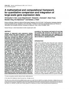
For other values of κ or for values of β in the interval (0, 1), (7) offers a wide range of feasible autocovariance structures in between, or even outside of, the ARMA and the FGN structures, as demonstrated in Figure 1(a), where we have plotted several autocovariance functions using different values of β, but keeping the same γ0, γ1 and γ2 for all cases. The meaning of the different values of β will be discussed later, in the end of this section. Here it may suffice to explain that GAS is more comprehensive than the FGN scheme as the latter, with its single parameter H, cannot model explicitly even the lag-one autocovariance. And it is also more comprehensive than ARMA schemes as it can explicitly model long-term persistence yet being parameter parsimonious. If the autocovariance is not everywhere positive but alternates in sign, (7) can be altered in agreement with (4) to become γj = γ0 (1 + κ β j)–1/β cos(θ0 + θ1 j)

(10)

In the form of (7) or (10), GAS has three or five parameters, respectively, one of which is the process variance γ0 (thus, the corresponding autocorrelation structure has two or four parameters, respectively). Although parameter parsimony is most frequently desired in stochastic modeling [e.g., Box and Jenkins, 1970, p. 17], GAS can be directly extended to include a greater number of parameters. Specifically, it can be assumed that the initial m + 1

9 terms γj (j = 0, …, m) have any arbitrary values (e.g. estimated from available records) and then (7) (or (10)) is used for extrapolating for large j. Essentially, this introduces m additional model parameters at most. Thus the total number of independent parameters is m + 1 if both κ and β are estimated in terms of γ0, …, γm, or m + 2 if β is estimated independently; even in the latter case κ cannot be regarded as an independent parameter because continuity at term γm demands that β

β1m γγm0  – 1‚ β > 0

κ=

m1 ln γγm0 ‚

(11) β=0

Parameter estimation can be based on the empirical autocovariance function. In the most parameter parsimonious model form (7), parameter γ0 is estimated from the sample variance and parameters κ and β can be estimated by fitting GAS to the empirical autocovariance function. There are several possibilities to fit these parameters: (a) We can chose to have a good overall fit to a number of autocovariances without preserving exactly any specific value. (b) Alternatively, we may choose to preserve exactly the lag-one autocovariance γ1 in which case (11) holds for m = 1. Still we have an extra degree of freedom (one more independent parameter), which can be estimated so as to get a good fit of GAS to autocovariances for a certain number of lags higher than one. (c) Finally, we may chose to preserve the lag-one and lag-two autocovariances exactly. Case (c) is the easiest to apply, as parameters κ and β are directly estimated from (7) in terms of γ0, γ1 and γ2. However cases (a) and (b) are preferable because they take into account the autocovariances of higher lags and, thus, the long memory properties of the process. A least squares method is a direct and simple basis to take into account more than two autocovariances in cases (a) and (b). Note that linearization of (7) by taking logarithms is not applicable as some empirical autocovariances may be negative. Therefore, the application of least squares requires nonlinear optimization, which is a rather

10 simple task as there are only two parameters in case (a) (κ and β) and one in case (b) (only β because of (11)). Results of applications of method (a) on synthetic and historical hydrologic data sets are given in Appendix A1. Apparently, parameter estimation is subject to high uncertainty, and this is particularly true for β, which is related to the long-term persistence of the process. Therefore, if the record length is small, it may be a good idea to assume a value of β after examining other series of nearby gauges, rather than to estimate it directly from the available small record. Similar parameter estimation strategies can be applied for the richer in parameters forms of GAS that were described above, in which case several values γj are preserved. We must emphasize that not any arbitrary sequence γj can be a feasible autocovariance sequence. Specifically, γj is a feasible autocovariance sequence if it is positive definite [Papoulis, 1991, pp. 293-294]. This can be tested in terms of the variance-covariance matrix h of the vector of variables [X1, …, Xs]T, which has size s  s and entries hij = γ|i – j|

(12)

If h is positive definite for any s then γj is a feasible autocovariance sequence. Normally, if the model autocovariances are estimated from data records, positive definiteness is satisfied. However, it is not uncommon to meet a case that does not satisfy this condition. The main reason is the fact that autocovariances of different lags are estimated using records of different lengths either due to the estimation algorithm (e.g., using (2)) or due to missing data. Another reason is the fact that, high lag autocovariances are very poorly estimated, as explained above. An alternative way to test that γj is a feasible autocovariance sequence is provided by the power spectrum of the process, which should be positive everywhere. The power spectrum of the process is the discrete Fourier transform (DFT; also termed the inverse finite Fourier transform) of the autocovariance sequence γj [e.g., Papoulis, 1991, pp. 118, 333; Bloomfield, 1976, pp. 46-49; Debnath, 1995, pp. 265-266; Spiegel, 1965, p. 175], that is

11 ∞

∞

j=1

j = –∞

sγ(ω) := 2 γ0 + 4  γj cos (2 π j ω) = 2  γj cos (2 π j ω)

(13)

Because γj is an even function of j (i.e., γj = γ–j), the DFT in (13) is a cosine transform; as usually we have assumed in (13) that the frequency ω ranges in [0, 1/2], so that γj is determined in terms of sγ(ω) by

1/2

γj =  sγ(ω) cos (2 π j ω) dω 

(14)

0

If autocovariance is given by the generalized relation (7) for all j, then it is easily shown that the power spectrum is

sγ(ω) = 2

where i :=

 γ0 –1 

1/β

1 + 2 β κ  

1     2iπω 1 Re Φ e ‚ ‚ β β κ   

(15)

–1, Re[ ] denotes the real part of a complex number, and Φ( ) is the Lerch

transcendent Phi function defined by zj Φ(z, b, a) :=  (a + j) b j=0 ∞

(16)

In the specific case that β = 0, where (8) holds, (15) reduces to (1 – e–2κ) sγ(ω) = 2 γ0 1 + e–2κ – 2 e–κ cos (2 π ω)

(17)

This gives a characteristic inverse S-shaped power spectrum (Figure 1(b)) that corresponds to a short memory process. Numerical investigation shows that for any β > 1 and κ = κ0 (given in (9)), (15) becomes approximately a power function of the frequency ω with exponent approaching 1/β – 1. (More

12 accurately, the exponent is by an amount δ smaller than 1/β – 1, where δ is about 0.03 for β ≥ 2.5 and decreases almost linearly to zero as β approaches 1. The exponent becomes almost equal to 1/β – 1 if κ is set equal to [1 + 0.71 ((1  1/β) (1 – 1 / 2β)] κ0; however in the latter case the departure of the power spectrum from the power law is greater). This case indicates a typical long memory process, similar to a FGN process (see Figure 1(b) where the power function appears as a straight line on the log-log plot). Generally, the power spectrum tends to infinity as ω tends to zero, regardless of the value of κ, if β ≥ 1. For β < 1 the power spectrum cannot be a power law of the frequency but approaches that given by (17) (inverse S-shaped) as β decreases, taking a finite value for ω = 0. If we fix γ0 and γ1 (the variance and the lag-one autocovariance) at some certain values, and vary β (and κ accordingly), we observe that there exists a combination of β = β* ≥ 1 and κ = κ0(β*) (given by (9)) resulting in a power spectrum s*(ω) approximately following a power law. For β > β* the power spectrum exceeds s*(ω) for low frequencies (that is, it departs from the straight line and becomes inverse J-shaped in the log-log plot). Τhe opposite happens if β < β* (the spectrum tends to the inverse S-shaped). This is demonstrated in Figure 1(b) where, in addition, γ2 has been also fixed; the power spectra of Figure 1(b) are those resulting from the autocovariances of Figure 1(a). Note that the power spectra of Figure 1(b) have been calculated numerically from (13) rather than from (15) because the three fixed autocovariances γ0, γ1 and γ2 do not allow a single instance of (7) to hold for all j. The case β = β* (straight line on log-log plot) that corresponds to the FGN process has been met in many hydrological and geophysical series. The case β = 0 (inverse S-shaped line on log-log plot) that corresponds to ARMA processes has been widely used in stochastic hydrology. In addition to these cases, the GAS scheme allows for all intermediate values of β in the range (0, β*), as well as for values β > β* (inverse J-shaped line on log-log plot, or very “fat” tail of autocovariance). The case 0 < β < β* implies a long-term persistence weaker than the typical FGN one. The case β > β* characterizes processes with strong long-term

13 persistence but not very strong lag-one correlation coefficient. Both these cases can be met in hydrologic series (see examples in Appendix A1). In Section 4.1 we will see how we can utilize the power spectrum of the process to determine the parameters of a generalized generating scheme, that will be introduced in the following section 3.

3

Description of the generating scheme It is well known [Box and Jenkins, 1970, p. 46] that, for any autocovariance sequence γj, Xi

can be written as the weighted sum of an infinite number of iid innovations Vi (also termed auxiliary or noise variables), that is, in the following form, known as (backward) moving average (BMA) form (where we have slightly modified the original notation of Box and Jenkins)

0

Xi =  a–j Vi + j = … + a2 Vi – 2 + a1 Vi – 1 + a0 Vi j = –∞

(18)

where aj are numerical coefficients that can be determined from the sequence of γj. Specifically, coefficients aj are related to γj through the equation [Box and Jenkins, 1970, pp. 48, 81]

∞

 aj ai + j = γi, i = 0, 1, 2, …

(19)

j=0

Although in theory Xi is expressed in terms of an infinite number of innovations, in practice it suffices to use a finite number of them for two reasons: (a) because the number of variables to be generated in any simulation problem is always a finite number, and (b) because terms a–j decrease as j → –∞ so that beyond a certain number j = –s all terms can be neglected without significant loss of accuracy. We must clarify that in our perspective, the number of non-

14 negative terms s + 1 is larger, by orders of magnitude, than p or q typically used in ARMA(p, q) models. Also, the number s is totally unrelated to the number of essential parameters m + 2 of the autocovariance function, discussed in section 2, as coefficients aj are internal parameters of the computational scheme. By contrast, the number s could be regarded as a large number of the order of magnitude 100 or 1000, depending on the decay of autocovariance, the desired accuracy, and the simulation length. In this respect, (18) and (19) can be approximated by

0

Xi =  a–j Vi + j = as Vi – s + … + a2 Vi – 2 + a1 Vi – 1 + a0 Vi j = –s

(20)

s–i

 aj ai + j = γi, i = 0, 1, 2, …

(21)

j=0

respectively, for a sufficiently large s. Extending this notion, we can write Xi as the weighted sum of both previous and next (theoretically infinite) innovation variables Vi, that is, in the following backward-forward moving average (BFMA) form

∞

Xi =  aj Vi + j = … + a–1 Vi – 1 + a0 Vi + a1 Vi + 1 + … j = –∞

(22)

where now the coefficients aj are related to γj through the almost obvious equation

∞

 aj ai + j = γi, i = 0, 1, 2, …

j = –∞

(23)

15 In section 5 we will see that the introduction of forward innovation terms (that is Vi + 1, Vi + 2, etc.) does not create any inconvenience even if the model is going to be used as a forecast model. The backward-forward moving average model (22) is more flexible than the typical backward moving average model (18). Indeed, the number of parameters aj in model (22) is double that of model (18) in order to represent the same number of autocovariances γj. Therefore, in model (22) there exists an infinite number of sequences aj satisfying (23). One of the infinite solutions of (23) is that with aj = 0 for every j < 0, in which case the model (22) is identical to the model (18). Another interesting special case of (22) is that with aj = a–j,

j = 1, 2, …

(24)

For reasons that will be explained below, the latter case will be adopted as the preferable model throughout this paper and will be referred to as the symmetric moving average (SMA) model (although the BMA model will be considered as well). In this case, (22) can be written as

s

Xi =  a|j| Vi + j = as Vi – s + … + a1 Vi – 1 + a0 Vi + a1 Vi + 1 + … + as Vi + s j = –s

(25)

where we have also restricted the number of innovation variables to a finite number, for the practical reasons already explained above. That is, we have assumed aj = 0 for |j| > s. The equations relating the coefficients aj to γj become now

s–i

 a|j| a|i + j| = γi,

j = –s

i = 0, 1, 2, …

(26)

Given that the internal model parameters aj are s + 1 in total, the model can preserve the first s + 1 terms of the autocovariance γj of the process Xi, if aj are calculated so that (26) is satisfied for i = 0, …, s. (In the next section we will discuss how this calculation can be done).

16 As we have already discussed, the number s can be chosen so that the desired accuracy can be achieved. The model implies non-zero autocovariance for a number of subsequent time lags. Thus, for the subsequent s terms (j = s + 1, …, 2s) the autocovariance terms are given by

s

γi =  aj ai – j, j=i–s

i = s + 1, …, 2s

(27)

(a consequence of (26) for i > s), whereas for even larger lags the autocovariance vanishes off. Apart from the parameters aj that are related to the autocovariance of the process Xi two more parameters are needed for the generating scheme, which are related to the mean and skewness of the process. These are the mean μV := E[Vi] and the coefficient of skewness ξV := E[(Vi – μV)3] of the innovations Vi (note that by definition Var[Vi] = 1). They are related to the corresponding parameters of Xi by  s    aj μV = μΧ, j = 0   

 s 3   a  ξV = ξΧ γ3/2 0  j = 0 j  

(28)

 3 s  a + 2  a3 ξV = ξΧ γ3/2 j 0  0 j=1   

(29)

for the BMA model and  s  a0 + 2  aj μV = μΧ,  j=1   

for the SMA model, which are direct consequences of (20) and (25), respectively. To provide a more practical view of the behavior of the SMA model, also in comparison with the typical BMA model, we demonstrate in Figure 2 two examples in graphical form. In the first example, we have assumed that the process Xi is Markovian with autocovariance (3) and γ0 = 1 and ρ = 0.9. In case of the BMA model with infinite aj terms, a theoretical solution of (19) is aj = γ0 (1 – ρ2) ρ j

(30)

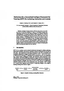
17 as it can be easily verified by substituting (30) to (19). If we choose to preserve the first 101 autocovariance terms γj assuming that aj = 0 for j > s = 100, we can numerically estimate from (21) the first 101 nonzero terms aj (in a manner that will be described in the next section). The numerically estimated aj are depicted in Figure 2(a); practically, they equal those given by (30), apart from the last three values which depart from theoretical values due to the effect of setting the high terms aj = 0 (the departure is clear in Figure 2(a)). The same autocovariance γj can be also preserved by the SMA model. The theoretical solution for infinite aj terms, and the approximate solution, again using 101 nonzero aj terms, are calculated from (23) and (26), respectively (using techniques that will be described in section 4), and are also shown in Figure 2(a). We observe that all aj values of the SMA model (apart from a0) are smaller than the corresponding aj values of the BMA model; for large j near 100, aj of the SMA model become one order of magnitude smaller than those of the BMA model. Apparently, this constitutes a strong advantage of the SMA model over the BMA one: the smaller the coefficients aj for large j, the smaller is the introduced error due to setting aj = 0 for j > s. In a second example we have assumed that Xi is a FGN process with autocovariance (5), and γ0 = 1 and H = 0.6 that corresponds to β = 1.25. This autocovariance is shown graphically in Figure 2(b) along with the resulting sequences of aj assuming again that the first 101 terms are nonzero. Once more we observe that the aj sequence of the SMA model lies below that of the BMA model. In addition to the approximate solution for 101 nonzero aj terms, a theoretical solution for infinite aj terms, also shown in Figure 2(b), is possible for the SMA model, as it will be described in section 4.1. We will also see in section 4.1 and Appendix A2 that a closed analytical solution is possible for the SMA model for any autocovariance γj, but not for the BMA model. This certainly constitutes a second advantage of the SMA model over the BMA one. As we have already mentioned above, the SMA model implies a nonzero autocovariance even for lags above the assumed numerical limit s, i.e., for j = s + 1 up to j = 2s, given by

18 (27). On the contrary, the BMA model implies that all autocovariance terms above s are zero. In Figure 3 we have plotted the resulting autocovariance of the above-described Markovian example for lags j up to 200. We observe that this structure may be an accepted approximation of the Markovian structure for lags 101 to 200 (at least it is better than the zero autocovariance implied by the BMA model). As this is achieved by no cost at all (no additional parameters are introduced), it can be regarded as an additional advantage of the SMA model over the BMA model. A fourth advantage of the SMA model is related to the preservation of skewness, in cases of skewed variables, which are very common in stochastic hydrology. It is well known [Todini, 1980; Koutsoyiannis, 1999a] that if the coefficient of skewness of the innovation variables becomes too high, it is impossible to preserve the skewness of the variables Xi. Therefore, the model resulting in lower coefficient of skewness of the innovation variables is preferable. In all cases examined, this was the SMA model. For instance, in the abovedescribed Markovian example, the SMA model resulted in ξV = 2.52 ξΧ whereas in the BMA model ξV = 3.27 ξΧ (by applying equations (29) and (28), respectively).

4

Computation of internal parameters of the generating scheme We will present two methods for computing the sequence of terms aj given the

autocovariance γj. The first method results in closed analytical solution of (23) for the case that (24) holds; this is applicable to the SMA model for an infinite number of aj terms. The second method is a numerical solution of (21) or (26) that determines a finite number of aj terms and is applicable to both the BMA and the SMA models.

4.1 Closed solution Denoting sa(ω) the DFT of the aj series and utilizing the convolution equation (23) and the fact that in the SMA model aj is an even function of j (equation (24)), we can show (see Appendix A2) that sa(ω) is related to the power spectrum of the process sγ(ω) by

19 sa(ω) = 2 sγ(ω)

(31)

This enables the direct calculation of the DFT of the aj series if the power spectrum of the process sγ(ω) (or equivalently, the autocovariance γj) is known. Then aj can be calculated by the inverse transform, i.e.,

1/2

aj =  sa(ω) cos (2 π j ω) dω 

(32)

0

Apart for few special cases, the calculations needed to evaluate aj from γj can be performed only numerically. However they are simple and non-iterative. In addition, all calculations can be performed using the fast Fourier transform (FFT, e.g., Bloomfield [1976, pp. 61-76]), thus enabling the building of a fast algorithm. For the BMA model, the fact that aj is not an even (nor an odd) function of j results in a complex DFT of aj. Therefore, the corresponding relation between sa(ω) and sγ(ω) becomes (see Appendix A2) |sa(ω)| = 2 sγ(ω)

(33)

where |sa(ω)| is the absolute value of sa(ω). Given that sa(ω) is complex, (33) does not suffice to calculate sa(ω) (it gives only its amplitude, not its phase). Therefore, the method cannot work for the BMA model. In addition, it is shown in Appendix 1 that there does not exist any other real valued transformation, different from DFT, that could result in an equation similar to (31) to enable a direct calculation of aj for the BMA model. However, the iterative method presented in section 4.2 can be applied to both the SMA and the BMA models.

20

4.2 Iterative solution The equations relating the model internal parameters aj to the autocovariance terms γj, i.e., equations (21) and (26) for the BMA and SMA model, respectively, may be written simultaneously for j = 0, …, s in matrix notation as pζ=θ

(34)

where ζ = [a0, …, as]T, θ = [γ0, …, γs]T (with the exponent T denoting the transpose of a matrix or vector) and p is a matrix with size (s + 1)  (s + 1) and elements pij = (1/2) [aj – i U(j – i) + ai + j – 2 U(s – i – j + 1)]

(35)

for the BMA model and pij = a|j – i| + ai + j – 2 U(j – 2) U(s – i – j + 1)

(36)

for the SMA model. Here U(x) is the Heaviside’s unit step function, with U(x) = 1 for x  0 and U(x) = 0 for x < 0. It can be easily verified that (35) and (36) (along with (34)) are equivalent to (21) and (26), respectively. Other expressions equivalent to (35) and (36) and simpler than them can be also derived, but (35) and (36) are the most convenient in subsequent steps. Clearly, each single equation of the system (34) includes second order products of unknown terms aj. Therefore, (34) may have one or more solutions in case of a positive definite autocovariance or no solution otherwise. Generally, we need to determine one single solution if it exists; otherwise, we may need to find the best approximation to (34). To accomplish these in a common manner, we reformulate the parameter estimation problem as a minimization problem, demanding to minimize f(ζ) = f(a0, …, as) := ||p ζ – θ||2 + λ (p1 ζ – γ0)2

(37)

21 where p1 is the first row of p, λ is a weighting factor and ||.|| denotes the Euclidean norm of a vector. The meaning of first term of the right hand side of (37) becomes obvious from (34). The second term denotes the square error in preserving the model variance γ0, multiplied by the weighting factor λ. Although, apparently, the second term is also contained in the first term, its separate appearance in the objective function enables its separate treatment. In case of a feasible autocovariance sequence, the minimum of f(ζ) will be zero, whatever the value of λ. However in case of an inconsistent autocovariance sequence the minimum of f(ζ) will be a positive number. In such a case the preservation of the variance γ0 is more important than that of autocovariance terms. Assigning a large value to λ (e.g., λ = 103), we force (p1 ζ – γ0)2 to take a value close to zero. Alternatively, λ could be considered as a Lagrange multiplier (an extra variable of the objective function (37)) but this would complicate the solution procedure. The task of minimization of f(ζ) is facilitated by determining its derivatives with respect to ζ. After algebraic manipulations it can be shown that d(p ζ) / dζ = 2 p (for both BMA and SMA schemes) so that d f(ζ) T dζ = 4 (p ζ – θ) p + 4 λ (p1 ζ – γ0) p1

(38)

Clearly, the problem we have to solve is an unconstrained nonlinear optimization problem with analytically determined derivatives. This can be easily tackled by typical methods of the literature such as the steepest descend and Fletcher-Reeves conjugate gradient methods [e.g., Mays and Tung, 1996, p. 6.12; Press et al., 1992, p. 422]. These are iterative methods, starting with an initial vector, which in our case can be taken as ζ[0] = [ γ0, 0, 0, …, 0]T, and iteratively improving it until the solution converges. The algorithm has been proven very quick and efficient in all cases examined, involving problems even with more than 1000 ai parameters. Examples of applying the algorithm for consistent autocovariances, Markovian and fractional Gaussian, have been already discussed

22 (Section 2 and Figure 2). An example of applying the algorithm to an inconsistent autocovariance is shown in Figure 4. The autocovariance of this example is identical to that of the Markovian example of Figure 2(a), apart from the values γ2 and γ3 that were both set equal to γ1; this creates a covariance matrix h not positive definite. As shown in Figure 4, the algorithm resulted in a very good approximation of the assumed autocovariance. In comparison with an earlier numerical procedure by Wilson [1969] (see also Box and Jenkins [1970, p. 203]) for determining the parameters of the BMA process, the above described algorithm is more general (it also covers the SMA case), faster (it does not involve matrix inversion, whereas Wilson’s algorithm does) and more flexible and efficient (can provide approximate solutions for inconsistent autocovariances, whereas Wilson’s algorithm cannot).

5

The generation scheme in forecast mode Equations (20) and (25) are directly applicable for simulation (unconditional generation) of

the process Xi. However, it is quite frequent the case where some of the variables Xi (past and present) are known and we wish either to generate other (future) variables, or to obtain best predictions of these (future) variables. As we will see, both problems can be tackled in a common simple manner, applicable for both the BMA and SMA models. We will assume that the vector consisting of the present and k past variables Z := [X0, X–1, …, X–k]T is known and its value is z = [x0, x–1, …, x–k]T. We wish either to generate any future variable Xj for j > 0, or to predict its value, under the condition Z = z. These can be done utilizing the following proposition, whose proof is given in Appendix 2: ~ Proposition: Let X i (i = –k, …, 0, 1, 2, … ) be any discrete time stochastic process with ~ ~ ~ ~ autocovariance γj (j = 0, 1, …) and let Z := [X 0, X –1, …, X –k]T. Let also Z := [X0, X–1, ~ …, X–k]T be a vector of stochastic variables independent of X i with mean and ~ autocovariance identical to that of X i. Then, the stochastic process

23 ~ ~ Xi = X i + ηiT h–1 (Z – Z), i = 1, 2, …

(39)

~ ~ ~ ~ where ηiT := Cov[ X i, Z] and h := Cov[Z, Z], has identical mean and autocovariance ~ with those of X i. In addition, the conditional variance of Xi given Z = z, is Var[Xi | Z = z] = γ0 – ηiT h–1 ηi

(40)

and is identical to the least mean square prediction error of Xi from Z. Note that h is a symmetric matrix with size (k + 1)  (k + 1) and elements given by (12) whereas ηi is a vector with size k + 1 and elements (ηi)j = γ|i + j – 1|

(41)

Also, note that the proposition is quite general and it can be applied to any type of linear stochastic model (not only to those examined in this paper). This proposition enables the following procedure for the forecast mode of the model: 1. Determine the matrix h using (12) for the given number (k + 1) of known (present and past) variables, and then calculate h–1. ~ 2. Generate a sequence of variables X i (i = –k, …, 0, 1, …), using the adopted model (20) or ~ (25) without any reference to the known variables Z. Form the vectors Z and Z, and ~ calculate the vector h–1 (Z – Z). 3. For each i > 0 determine the vector ηi from (41) and calculate the final value of the variable Xi, conditional on Z, from (39). Equation (40) shows that the conditional variance of Xi is smaller than the unconditional one (γ0), as expected. The fact that this conditional variance is identical to the least mean square prediction error of Xi from Z, ensures us that no further reduction is possible by any type of linear prediction model. Thus, the combination of model (20) or (25) with the

24 transformation (39) allows preservation of the stochastic structure of the process, whatever this structure is, and simultaneously reduces the conditional variance to its smallest possible value, in the sense that no other linear stochastic model could reduce it further. Notably, the same generating model (20) or (25) is used in both modes, simulation and forecast. Theoretically, the procedure can be applied to negative values of i, as well. In this case, if k ≤ i ≤ 0, it is easy to show that (39) reduces to the trivial case Xi = Xi, as it should (see Appendix 2). The above steps are appropriate if the forecast is done in terms of conditional simulation. If it must be done in terms of expected values rather than conditionally simulated values, then in ~ step 2 of the above procedure, X i are set equal to their (unconditional) expected values rather than generated. In this case, if confidence limits are needed, they can be calculated in terms of the conditional variance given by (40).

6

Multivariate case The model studied in the previous sections is a single variate model but can be easily

extended to the multivariate case. In this case the model, apart from the temporal covariance structure, should consider and preserve the contemporaneous covariance structure of several variables corresponding to different locations. Let Xi = [X i1, X i2, …, X in]T be the vector of n stochastic variables each corresponding to some location specified by the index l = 1, , n, at a specific time period i. Let also g be the variance-covariance matrix of those variables with elements glk := Cov[X il, X ik], l, k = 1, 2, …, n

(42)

We assume that each of the variables X il can be expressed in terms of some auxiliary variables V il (again with unit variance) by using either

25 0

X il =  a–rl Vil+ r,

(43)

r = –s

for the BMA model, or s

X il =  a|r|l Vil+ r

(44)

r = –s

for the SMA model. These equations are similar to (20) and (25), respectively. The auxiliary variables V il can be assumed uncorrelated in time i (i.e., Cov[V il, Vmk] = 0 if i ≠ m) but correlated in different locations l for the same time i. If c is the variance-covariance matrix of variables V il, then each of its elements clk := Cov[V il, V ik], l, k = 1, 2, …, n

(45)

can be expressed in terms of glk and the series of ali and aki by

clk = glk

/

s

 arl akr

(46)

r=0

for the BMA model and clk = glk

/

s

 a|r|l a|r|k

(47)

r = –s

for the SMA model. These equations are direct consequences of (43) and (44), respectively. The theoretically anticipated lagged cross-covariance for any lag j = 0, 1, ..., is then

s–j

Cov[X il, Xik+ j] = glk  arl akj + r r=0

for the BMA model and

/

s

 arl akr

r=0

(48)

26 s–j

Cov[X il, Xik+ j] = glk  al|j + r| a|r|k r = –s

/

s

 a|r|l a|r|k

r = –s

(49)

for the SMA model. Given the variance-covariance matrix c, the vector of variables Vi = [V i1, V i2, …, V in]T can be generated using the simple multivariate model Vi = b Wi

(50)

where Wi = [W i1, W i2, …, W in]T is a vector with innovation variables with unit variance independent both in time i and in location l = 1, …, n, and b is a matrix with size n  n such that b bT = c

(51)

The methodology for solving (51) for b given c (also known as taking the square root of c) will be discussed in section 7 below. The other parameters needed to completely define model (50) are the vector of mean values μW and coefficients of skewness ξW of W il. These can be calculated in terms of the corresponding vectors μV and ξV of V il, already known from (28) or (29), by μW = b–1 μV,

ξW = (b(3))–1 ξV

(52)

which are direct consequences of (50). In (52), b(3) is the matrix whose elements are the cubes of b and the exponent –1 denotes the inverse of a matrix. To illustrate the method we have applied it to a problem with two locations with statistics given in Table 1. To investigate the method’s ability to preserve long-term memory properties such as the Hurst coefficient in multiple dimensions we have assumed the FGN structure with exponents β equal to 1.25 and 1.667 for locations 1 and 2, respectively, corresponding to Hurst coefficients 0.6 and 0.7 for locations 1 and 2, respectively. We generated a synthetic

27 record with 10 000 data values using the SMA scheme with 2 000 nonzero aj terms, which were evaluated by the closed solution described in section 4.1. The last (2000th) term of the series of aj was 610–5 a0 for location 1 and 3104 a0 for location 2; these small values indicate that the error due to neglecting the higher aj terms (beyond term 2000) is small. The required computer time on a modest (300 MHz) Pentium PC was about 10 seconds for the computation of internal parameters (when the fast Fourier transform was implemented in the algorithm; otherwise it increased to about 2 minutes) and other 10 seconds for the generation of the synthetic records. As shown in Table 1, the preservation of all statistics was perfect. In addition, Figure 5 shows that the autocorrelation and cross-correlation function, the power spectrum, and the rescaled range as a function of record length were very well preserved, as well.

7

Finite length of autocorrelation sequence In all above sections it was assumed that the autocovariance γj is defined for any arbitrarily

high lag j. However, there are cases where only a finite number of autocovariance terms can be defined. For example in a stochastic model describing rainfall increments at time intervals δ within a rainfall event with certain duration d = q δ (where q is an integer), the autocovariance has no meaning for lags greater than q – 1 (see the application in the end of this section). Such cases can be tackled in a different, rather simpler, way. An appropriate model for this case is X=bV

(53)

where X = [X1, …, Xq]T is the vector of variables to be modeled with variance-covariance matrix h given by (12), V = [V1, …, Vq]T is a vector of innovations with unit variance, and b is a square matrix of coefficients with size q  q. The main difference from the models of previous sections is that the number of innovations V equals the number q of the modeled

28 variables X (the length of the synthetic record). In this case the distributions of innovations V cannot be identical. Each one has different mean and coefficient of skewness, given by μV = b–1 μX,

ξV = (b(3))–1 ξX

(54)

which are direct consequences of (53). The matrix of coefficients b is given by b bT = h

(55)

which again is a direct consequence of (53). It is reminded that (55) has an infinite number of solutions b if h is positive definite. Traditionally, two well-known algorithms are used which result in two different solutions b (see. e.g., Bras and Rodriguez-Iturbe [1985, p. 96]; Koutsoyiannis [1999a]). The first and simpler algorithm, known as triangular or Cholesky decomposition, results in a lower triangular b. The second, known as singular value decomposition, results in a full b using the eigenvalues and eigenvectors of h. A third algorithm has been proposed by Koutsoyiannis [1999a] which is based on an optimization framework and can determine any number of solutions, depending on the objective set (for example, the minimization of skewness, or the best approximation of the covariance matrix, in case that it is not positive definite). We can observe that the lower triangular b is directly associated to the BMA model discussed above, but with different number of innovations Vi for each Xi. Thus, if b is lower triangular, then apparently X1 = b11 V1, X2 = b21 V1 + b22 V2, etc. Likewise, a symmetric b is associated to the SMA model. An iterative method for deriving a symmetric b can be formulated as a special case of the methodology proposed by Koutsoyiannis [1999a]. This can be based on the minimization of f(b) := ||b bT – h||2

(56)

where we have used the notation ||b bT – h|| for the norm (more specifically, we adopt the Euclidean or standard norm here; see, e.g., Marlow [1993, p. 59]), as if b bT – h were a vector

29 in q2 space rather than a matrix. The derivatives of f(b) with respect to b are easy to determine (see Appendix 3). Using the notation dα / db =[∂α / ∂bij] for the matrix of partial derivatives of any scalar a with respect to all bij (this is an extension of the notation used for vectors, e.g., Marlow [1993, p. 208]) and considering that b is symmetric we find that d f(b) * db = 8 e – 4 e

(57)

where e := (b bT – h) b and e* = diag(e11, e22, …, eqq), that is a diagonal matrix containing the diagonal elements of e. As in the similar case of section 4.2, the problem here is an unconstrained nonlinear optimization problem with analytically determined derivatives, which can be easily tackled by typical methods such as the steepest descend and the Fletcher-Reeves conjugate gradient methods. As initial solution for the iterative procedure we should use a symmetric one; a good choice is b[0] = γ0 I, where I is the identity matrix. To illustrate the method and the differences among the three different solutions discussed, we have considered a stochastic model of a rainfall event with duration d = 20 h using a halfhour time resolution δ, so that the number of variables is q = 20 / 0.5 = 40. We denote Xi (i = 1, …, 40) the half-hour rainfall increments and assume that the covariance structure of Xi is as in the Scaling Model of Storm Hyetograph [Koutsoyiannis and Foufoula-Georgiou, 1993], that is γ|i – j| = Cov[Xi, Xj] = [(c2 + c12) φ(|j – i|, β) q 1/β – c12] (d 2(κ + 1) / q 2)

(58)

where c1, c2, κ and β are parameters and φ(m, β) := (1/2) [(m – 1)2 – 1/β + (m + 1) 2 – 1/β] – m2 – 1/β,

m>0

(59)

whereas φ(0, β) = 1. This is apparently a long memory autocorrelation structure similar to the FGN structure. It always results in consistent (positive definite) autocovariance if it is

30 evaluated within the duration d of the event; however for certain combinations of parameters it can result in inconsistent autocovariance values if it is attempted to evaluate it outside of the event (i.e., for lags greater than q – 1). For the example presented here we have assumed that the model parameters are c1 = 8.74, c2 = 85.68, κ = –0.45 and β = 10 (units mm and h). The statistics of Xi, determined from equations given by Koutsoyiannis and Foufoula-Georgiou [1993], are μX = 1.14 mm, γ0 = 2.68 mm2 and ξX = 2.88 (the latter is determined assuming two parameter gamma distribution for Xi). The matrix b is 40  40 (1600 elements). We have calculated all three solutions of the matrix b described above (triangular, singular value, and symmetric) which are shown schematically in Figure 6. We observe a regular pattern with a strong diagonal and a strong first column for the triangular solution, a strong first column and an irregular pattern for other columns for the singular value solution, and a regular pattern with a strong diagonal for the symmetric solution. An appropriate means to compare the three solutions is provided by the resulting coefficients of skewness of innovations Vi, given by (54). These are shown in Figure 7. The singular value solution resulted in coefficients of skewness ranging from –40 to +62, which apparently are computationally intractable at generation. More reasonable are the values of the triangular solution, with a maximum coefficient of skewness equal to about 10. The symmetric solution resulted in the smallest, among the three cases, maximum coefficient of skewness, slightly exceeding 6. Notably, this value is the smallest possible value among all possible (infinite) b solutions of (55) [Koutsoyiannis, 1999b]. This enhances further the already discussed feature of the SMA model, that symmetric solutions result in smaller coefficients of skewness of innovations, a feature quite expedient in stochastic hydrology. The finite length scheme described in this section can be a preferable alternative even in cases where the autocovariance is defined for any j, but the length q of the synthetic record is very small. Specifically, the scheme of the present section 7 uses q2 internal parameters. In

31 case that the process exhibits long memory, the required number of parameters s of the schemes of section 3 may be greater than q2, and, thus, the scheme of section 7 could be preferable.

8

Summary, conclusions and discussion The main topics of the proposed framework can be summarized in the following points:

1. A generalized autocovariance function is introduced which unifies in a simple mathematical expression both short memory (ARMA) and long memory (FGN) models, considering them as special instances in a parametrically defined continuum, more comprehensive than these classes of models. 2. A moving average stochastic generation scheme is proposed that can implement the generalized autocovariance function (or any other autocovariance function). In addition to the traditional backward moving average scheme, a new time symmetric (backwardforward) moving average scheme is proposed. It is computationally more convenient and also results in better treatment of processes with skewed distributions. 3. Two methods of determining the internal parameters of the generating scheme are proposed. The first is a closed method based on the power spectrum of the process and applicable to the symmetric moving average scheme. The second is an iterative method based on convolution equations and applicable to both instances of the generating scheme. 4. The proposed stochastic generation scheme is directly adaptable so as to perform in forecast mode. To this aim a generalized adaptation methodology is studied, applicable to any type of stochastic model. 5. The model can perform in single-variate as well as in multivariate problems. 6. A specific form of the model for problems where the autocorrelation function can be defined only for a certain finite number of lags (e.g., in generation of rainfall increments within a rainfall event) is also studied. An incidental contribution of this study is a method

32 for determining a symmetric square root of a symmetric matrix; this symmetric square root is the direct analogue of the symmetric moving average generating scheme and, as demonstrated by an example, it outperformed non-symmetrical solutions. Thus, the proposed framework is a generalized tool for any kind of single-variate and multivariate simulation and forecasting problems in stochastic hydrology involving stationary stochastic processes. We emphasize its appropriateness for modeling long memory processes and its ability for preserving the Hurst coefficients in multivariate processes, even if each location has a different Hurst coefficient. Simultaneously, it enables explicit preservation of the skewness of the processes (at no computational or other cost, apart from generating skewed rather than Gaussian random numbers), a feature that is of major concern in stochastic hydrology. Owing to the proposed fast algorithms for computation of internal parameters, the required computing time is small, even for problems including thousands of such parameters. In traditional stochastic models, three different issues, i.e., the type of the generation scheme, the number of model parameters, and the type of autocovariance, are merged in one. For example, if we choose the AR(1) model as a generation scheme, we simultaneously choose to use two second order parameters (variance and lag-one autocovariance), and assume that the autocovariance is an exponential function of the lag. In our approach, we have separated these three issues. The autocovariance function has a single mathematical expression of power type. The number of parameters can be decided separately, depending on the desired parsimony or non-parsimony of parameters and the length of the available record. The minimum number of parameters is three, one being the variance and another one the exponent of the power type autocovariance function. This exponent equals zero for the model with the shortest possible memory, and becomes greater than one for a long memory model. Coming then to the generation scheme, this has a mathematical expression independent of the autocorrelation function. What we have to decide here is the number of innovation terms,

33 which depends on the length of the synthetic record to be generated, the desired accuracy, and the adopted decay of autocorrelation. In its present form, the proposed framework is formulated for stationary processes. Therefore, it can be directly used, for modeling of annual flows or short time scale problems (e.g., rainfall generation within a rainfall event) that are not affected by seasonality. Thus, it is not appropriate for problems involving periodic processes (e.g., seasonal flows). However, it can be directly linked to seasonal short memory models such as the PAR(1) single-variate or multivariate model to simulate seasonal processes, as well. Such a linkage of annual to seasonal models has been studied elsewhere [Koutsoyiannis and Manetas, 1996]. The combination of an annual long memory model and a seasonal model will preserve both the long term memory properties, which will be indirectly transferred from the annual time scale into the seasonal time scale, and the seasonal properties. In addition, any other annual-toseasonal disaggregation model [Salas et al., 1980; Stedinger and Vogel, 1984; Grygier and Stedinger, 1988, 1990; Lane and Frevert, 1990] could also be combined with the annual model in this respect.

34

Acknowledgments. The research leading to this paper was performed within the framework of the project Modernization of the supervision and management of the water resource system of Athens, funded by the Water Supply and Sewage Corporation of Athens. The author wishes to thank the director I. Nazlopoulos, the associate director A. Xanthakis, and the members of the project committee for the support of the research. Thanks are also due to A. Efstratiadis for his comments and testing of the methodology. Finally, the author is grateful to the Associate Editor P. Kumar, the reviewers C. Puente and A. Carsteanu, and an anonymous reviewer, for their constructive comments that were very helpful for an improved, more complete and more accurate presentation.

35

References Barnes, F. B., Storage required for a city water supply, J. Inst. Eng. Australia, 26(9) 198-203, 1954. Beard, L. R., Use of interrelated records to simulate streamflow, Proc. ASCE, J. Hydraul. Div., 91(HY5), 13-22, 1965. Bloomfield, P., Fourier Analysis of Time Series, Wiley, New York, 1976. Box, G. E. P., and G. M. Jenkins, Time series analysis; Forecasting and control, Holden Day, 1970. Bras, R.L. and I. Rodriguez-Iturbe, Random functions in hydrology, Addison-Wesley, 1985. Debnath, L., Integral Transforms and Their Applications, CRC Press, New York, 1995. Ditlevsen, O. D., Extremes and first passage times, Doctoral dissertation presented to the Technical University of Denmark, Lyngby, Denmark, 1971. Eckhardt, R., Stan Ulam, John von Neumann and the Monte Carlo method, in From cardinals to chaos, ed. by N. G. Cooper, Cambridge University, NY., 1989. Grygier, J. C. and Stedinger, J. R., Condensed disaggregation procedures and conservation corrections for stochastic hydrology, Water Resour. Res., 24(10), 1574-1584, 1988. Grygier, J. C. and J. R. Stedinger, SPIGOT, A synthetic streamflow generation software package, Technical description, School of Civil and Environmental Engineering, Cornell University, Ithaca, NY., Version 2.5, 1990. Hurst, H. E., Long-term storage capacity of reservoirs, Trans. Am. Soc. Civ. Eng., 116, 776808, 1951. Koutsoyiannis, D., Optimal decomposition of covariance matrices for multivariate stochastic models in hydrology, Water Resour. Res., 35(4), 1219-1229, 1999a. Koutsoyiannis, D., An advanced method for preserving skewness in single-variate, multivariate and disaggregation models in stochastic hydrology, XXIV General

36 Assembly of European Geophysical Society, The Hague, Geophys. Res. Abstracts, 1(1), p. 346, 1999b. (Presentation available on line at http://www.hydro.ntua.gr/faculty/dk/ pub/pskewness.pdf) Koutsoyiannis, D., and E. Foufoula-Georgiou, A scaling model of storm hyetograph, Water Resour. Res., 29(7), 2345-2361, 1993. Koutsoyiannis, D., and A. Manetas, Simple disaggregation by accurate adjusting procedures, Water Resources Research, 32(7), 2105-2117, 1996 Lane, W. L. and D. K. Frevert, Applied Stochastic Techniques, User’s Manual, Bureau of Reclamation, Engineering and Research Center, Denver, Co., Personal Computer Version 1990. Maass, A., M. M. Hufschmidt, R. Dorfman, H. A. Thomas, Jr., S. A. Marglin, and G. M. Fair, Design of Water Resource Systems, Harvard Univerity Press, Cambridge, Mass., 1962. Mandelbrot, B. B., Une class de processus stochastiques homothetiques a soi: Application a la loi climatologique de H. E. Hurst, Compte Rendus Academie Science, 260, 3284-3277, 1965. Mandelbrot, B. B., A fast fractional Gaussian noise generator, Water Resour. Res., 7(3), 543553, 1971. Mandelbrot, B. B., and J. R. Wallis, Computer experiments with fractional Gaussian noises, Part 1, Averages and variances, Water Resour. Res., 5(1), 228-241, 1969a. Mandelbrot, B. B., and J. R. Wallis, Computer experiments with fractional Gaussian noises, Part 2, Rescaled ranges and spectra, Water Resour. Res., 5(1), 242-259, 1969b. Mandelbrot, B. B., and J. R. Wallis, Computer experiments with fractional Gaussian noises, Part 3, Mathematical appendix, Water Resour. Res., 5(1), 260-267, 1969c. Marlow, W. H., Mathematics for Operations Research, Dover Publications, New York, 1993. Matalas, N. C., Mathematical assessment of synthetic hydrology, Water Resour. Res., 3(4), 937-945, 1967.

37 Matalas, N. C. and J. R. Wallis, Generation of synthetic flow sequences, in Systems Approach to Water Management, edited by A. K. Biswas, McGraw-Hill, New York, 1976. Mays, L. W., and Y.-K. Tung, Systems analysis, in Water Resources Handbook, edited by L. W. Mays, McGraw-Hill, New York, 1996. McLeod, T. A., and K. W. Hipel, Simulation procedures for Box-Jenkins models, Water Resour. Res., 14(5), 969-975, 1978. Mejia, J. M., I. Rodriguez-Iturbe and D. R. Dawdy, Streamflow simulation, 2, The broken line process as a potential model for hydrologic simulation, Water Resour. Res., 8(4), 931941, 1972. Metropolis, N., The beginning of the Monte Carlo method, in From cardinals to chaos, ed. by N. G. Cooper, Cambridge University, NY., 1989. O’Connell, P. E., Stochastic Modelling of Long-Term Persistence in Streamflow Sequences, PhD thesis presented to the Civil Engineering Department, Imperial College, London, 1974. Papoulis, A., Probability, Random Variables, and Stochastic Processes, 3rd ed., McGraw-Hill, New York, 1991. Press, W. H., S. A. Teukolsky, W. T. Vetterling, and B. P. Flannery, Numerical Recipes in C, Cambridge University Press, Cambridge, 1992. Salas, J. D., Analysis and modeling of hydrologic time series, Chapter 19, Handbook of hydrology, edited by D. Maidment, McGraw-Hill, New York, 1993. Salas, J. D., J. W. Delleur, V. Yevjevich, and W. L. Lane, Applied Modeling of Hydrologic Time Series, Water Resources Publications, Littleton, Colo. 1980. Spiegel, M. R., Theory and Problems of Laplace Transforms, Shaum, New York, 1965. Stedinger, J. R., and R. M. Vogel, Disaggregation procedures for generating serially correlated flow vectors, Water Resour. Res., 20(1) 47-56, 1984.

38 Thomas, H. A., and M. B. Fiering, Mathematical synthesis of streamflow sequences for the analysis of river basins by simulation, in Design of Water Resource Systems, by A. Maass, M. M. Hufschmidt, R. Dorfman, H. A. Thomas, Jr., S. A. Marglin, and G. M. Fair, Harvard Univerity Press, Cambridge, Mass., 1962. Todini, E., The preservation of skewness in linear disaggregation schemes, J. Hydrol., 47, 199-214, 1980. Wilson, G. J., Factorization of the generating function of a pure moving average process, SIAM Jour. Num. Analysis, 6, 1, 1969.

39

List of Figures

Figure 1 (a) Examples of autocovariance sequences of the proposed generalized type for several values of the exponent β, in comparison with the fractional Gaussian noise and ARMA types; (b) corresponding power spectra. Figure 2 Two examples of theoretical autocovariance sequences and resulting sequences of internal parameters aj for BMA and SMA schemes: (a) a Markovian autocovariance sequence; (b) a Fractional Gaussian noise autocovariance sequence. The obtained autocovariance sequences by either of the BMA or SMA schemes are indistinguishable from the theoretical ones. Figure 3 Obtained autocovariance structure from the SMA scheme using 100 aj terms, for lags 0-200; the theoretical autocovariance structure is that of Figure 2(a). Figure 4 An example of an inconsistent γj sequence approximated with a consistent sequence achieved by the SMA scheme using 100 aj terms; the latter are also plotted, in comparison with the corresponding terms of the BMA scheme. Figure 5 Preservation of statistical properties by the simulated records of the application of section 6: (a) autocovariance; (b) power spectra; (c) rescaled range and Hurst coefficients; (d) cross-covariance. Figure 6 Comparison of three different solutions of parameter matrices b (3-D plots of their elements) of the application of section 7: (a) triangular solution; (b) singular value solution; (c) symmetric solution. Figure 7 Comparison of the resulting coefficients of skewness of the 40 innovations of the application of section 7 for the three different solutions of parameter matrices b.

40

Table 1 Theoretical and empirical statistics of the application of section 6.

Theoretical Location 1

Location 2

Empirical Location 1 Location 2

Mean

1.00

2.00

1.00

1.97

Standard deviation

0.50

1.20

0.51

1.21

Coefficient of skewness

1.00

1.20

1.03

1.14

Hurst coefficient

0.60

0.70

0.61

0.71

Cross correlation coefficient

0.70

0.70

Autocovariance, γj

41

1

β = 2.5

(a)

Generalized autocovariance Fractional Gaussian noise

β = 1.25

0.1 0.01 0.001

β = 0.5

β =1

0.0001 1E-04 0.00001 1E-05

β = 0.25

0.000001 1E-06 0.0000001 1E-07 0.00000001 1E-08

β = 0 (ARMA)

0.000000001 1E-09

β = 0.125

1E-10 1E-10 0

10

20

30

40

50

60

70

80

90

100

ln sγ (ω )

Lag, j 1.8

β = 2.5 β = 1.25

1.6 1.4

(b)

Generalized autocovariance Fractional Gaussian noise

β = 1 β = 0.5 β = 0.25

1.2

1 β = 0.125 β = 0 (ARMA) 0.8 0.6 0.4 -6

-5

-4

-3

-2

-1

ln ω

0

Figure 1 (a) Examples of autocovariance sequences of the proposed generalized type for several values of the exponent β, in comparison with the fractional Gaussian noise and ARMA types; (b) corresponding power spectra.

BMA and SMA parameters, a j

Autocovariance, γ j

42

1 (a) 0.1 0.01 0.001 0.0001 Autocovariance BMA parameters, 100 terms BMA parameters, infinite terms SMA parameters, 100 terms SMA parameters, infinite terms

0.00001 0.000001 0

20

40

60

80

100

BMA and SMA parameters, a j

Autocovariance, γ j

Sequence term, j

1 (b)

0.1

0.01

0.001

Autocovariance BMA parameters, 100 terms SMA parameters, 100 terms SMA parameters, infinite terms

0.0001 0

20

40

60

80 100 Sequence term, j

Figure 2 Two examples of theoretical autocovariance sequences and resulting sequences of internal parameters aj for BMA and SMA schemes: (a) a Markovian autocovariance sequence; (b) a Fractional Gaussian noise autocovariance sequence. The obtained autocovariance sequences by either of the BMA or SMA schemes are indistinguishable from the theoretical ones.

Autocovariance, γ j

43

1 0.1 0.01 0.001 0.0001 1E-05 1E-06 1E-07 1E-08 1E-09 Theoretical Obtained from SMA with 100 terms

1E-10 1E-11 0

50

100

150

200 Lag, j

Figure 3 Obtained autocovariance structure from the SMA scheme using 100 aj terms, for lags 0-200; the theoretical autocovariance structure is that of Figure 2(a).

BMA and SMA parameters, a j

Autocovariance, γ j

44

1 0.1 0.01 0.001 0.0001 Autocovariance, inconsistent Autocovariance, achieved by SMA BMA parameters, 100 terms SMA parameters, 100 terms

0.00001 0.000001 0

20

40

60

80 100 Sequence term, j

Figure 4 An example of an inconsistent γj sequence approximated with a consistent sequence achieved by the SMA scheme using 100 aj terms; the latter are also plotted, in comparison with the corresponding terms of the BMA scheme.

Autocovariance, γ j

45 0.40 0.35 0.30 0.25 0.20 0.15 0.10

(a )

Theoretical Simulated Location 1

Location 2

0.05 0.00 -0.05

ln s γ (ω )

0

20

40

60

80

3.50

Lag, j 100 (b)

2.50

Theoretical Simulated

Location 2

1.50 0.50

Location 1

-0.50 -1.50

Log (Rescaled range)

-4.5

-4.0

-3.5

-3.0

-2.5

-2.0

-1.5

-1.0

-0.5 0.0 ln ω

3.0 (c)

Slope (Hurst coefficient) = 0.5 0.6 0.7

2.5 2.0 1.5 1.0

Empirical, location 1

0.5

Empirical, location 2

0.0

C ross-covariance

1.0

1.5

2.0

2.5

3.0

3.5 4.0 Log (Record length)

0.30 (d)

0.25 Theoretical Simulated

0.20 0.15 0.10 0.05 0.00

-0.05 -100

-80

-60

-40

-20

0

20

40

60

80 100 Lag, j

Figure 5 Preservation of statistical properties by the simulated records of the application of section 6: (a) autocovariance; (b) power spectra; (c) rescaled range and Hurst coefficients; (d) cross-covariance.

46

0.8 0.6

aij

0.4 0.2 0

(a)

10 10

20

20

j

30

30

i

40

0.8 0.6 0.4

aij 0.2 0 - 0.2

(b)

10 10

20

20

j

30

30

i

40

0.8 0.6

aij

0.4 0.2 0

(c)

10 10

20

20

j

30

30

i

40

Figure 6 Comparison of three different solutions of parameter matrices b (3-D plots of their elements) of the application of section 7: (a) triangular solution; (b) singular value solution; (c) symmetric solution.

47

64 62 60 10

Coefficient of skewness ξVi

8 6 Triangular Singular value Symmetric

4 2 0 -2 -4 -6 -8 -10 -36 -38 -40 0

5

10

15

20

25

30

35

40

Variable number, i

Figure 7 Comparison of the resulting coefficients of skewness of the 40 innovations of the application of section 7 for the three different solutions of parameter matrices b.

A generalized mathematical framework for stochastic simulation and forecast of hydrologic time series Demetris Koutsoyiannis Department of Water Resources, Faculty of Civil Engineering, National Technical University, Athens Heroon Polytechneiou 5, GR-157 80 Zographou, Greece ([email protected])

Appendix (Supplement on microfiche)

A1 Some examples for comparison of the generalized autocovariance structure to fractional Gaussian noise models In this Appendix, we demonstrate the generalized autocovariance structure (GAS; Equation (7)) using synthetic and historical data records, also comparing it with the stochastic structure implied by the fractional Gaussian noise (FGN) model. We give five examples with record lengths between 44 and 100. The first two of them are synthetic samples generated by stochastic models. In this case the theoretical autocovariance function is known and, consequently, we can test the ability of model to capture this stochastic structure, and the appropriateness of the fitting method. The other three examples are annual streamflow and rainfall records of gauges at Greece and USA. In this case our purpose is to compare the appropriateness of each of the GAS and FGN models for fitting the data and investigate the model parameters. For the GAS case, the most parameter parsimonious form was adopted for all examples, using the parameters γ0, β and κ only. The fitting of β and κ was done by the least squares method on the empirical autocorrelation function (see section 2) for lags 0-20. The same method was used for the FGN case as well (symbolically, FGN/A). Fitting by means of the Husrt coefficient was also performed as an alternative for the FGN case (symbolically, FGN/H). The results are presented in graphical form in terms of autocorrelation functions and power spectra in Figure A1 through Figure A5. AR(1) example. 100 data values were generated using a Gaussian AR(1) process with unit variance and lag-one autocorrelation coefficient equal to 0.5. In this case, the theoretical autocovariance function has the form (8). The fitted parameters for the GAS case are β = 0.01

2 (very close to the theoretical value 0) and κ = 0.66. The resulting autocorrelation function and power spectrum are almost identical to the theoretical ones. Apparently, the FGN model is not appropriate for this case since we know that the process is not long memory at all. Had we only the data record available, without knowing the theoretical autocorrelation, we possibly attempt to fit the FGN model. Then, applying the least squares method (FGN/A) we would find β = 1.31 (H = 0.62), which clearly underestimates the autocorrelation for small lags and overestimates it for large lags. Applying the Hurst coefficient method we would find H = 0.44 which would interpret as H = 0.5 (values smaller than 0.5 are not allowed by FGN) and we

Autocorrelation, ρj

would assume that the process is white noise, which is not correct. 1 Theoretical Empirical GAS FGN/A FGN/H

0.8 0.6 0.4

(a)

0.2 0 -0.2 -0.4

ln sρ (ω )

0

5

10

15

20

Lag, j

2

(b)

1.5 1 0.5 0

Theoretical Empirical GAS FGN/A FGN/H

-0.5 -1 -1.5 -4

-3

-2

-1

ln ω

0

Figure A1 Comparison of theoretical, empirical and fitted model autocorrelation functions (a) and power spectra (b) for a synthetic data set generated by an AR(1) process with 100 values.

3 FGN example. 100 data values were picked from the synthetic record generated in the application of section 6 (location 2). In this case, the theoretical autocovariance function has the form (5) with H = 0.7. The fitted parameters for the GAS case are β = 1.48 (>1, close to the theoretical value β = 1 / [2(1 – H)] = 1.67) and κ = 3.28. The resulting autocorrelation function and power spectrum are almost identical to the theoretical ones. The fitted parameter for the FGN/A case is β = 1.67 (H = 0.70), which is identical to the theoretical ones. However, applying the Hurst coefficient method we find H = 0.98, which is too high and results in autocorrelation function and power spectrum extremely departing from both the

Autocorrelation, ρj

theoretical and empirical ones. 1

(a)

0.8 Theoretical Empirical GAS FGN/A FGN/H

0.6 0.4 0.2 0 -0.2

ln sρ (ω )

0

5

10

15

Lag, j

20

2

(b)

1.5 1 0.5 0 -0.5 -1 -1.5

Theoretical Empirical GAS FGN/A FGN/H

-2 -2.5 -3 -4

-3

-2

-1

ln ω

0

Figure A2 Comparison of theoretical, empirical and fitted model autocorrelation functions (a) and power spectra (b) for a synthetic data set generated by a FGN process with 100 values.

4 Kremasta streamflow example. In this example we used a 44-year annual streamflow record of Acheloos River at Kremasta dam (Western Greece; overyear annual discharge 117.9 m 3/s). The estimated Hurst coefficient of the series is as high as 0.94, indicating a long memory. The fitted parameters for the GAS case are β = 2.43 and κ = 12.6, and, indeed, indicate a very long memory. Note that for empirical lag-one autocorrelation ρ1 = 0.22, the characteristic parameter β* defined in section 2 is 1.54 and thus β > β*. The fitted parameter for the FGN/A case is β = 1.75 (H = 0.71 < 0.94). Both GAS and FGN/A schemes agree well with the empirical autocorrelations and power spectra, the former outperforming the latter as better approaching the lag-one autocorrelation, which is important. The FGN/H scheme again results

Autocorrelation, ρj

in autocorrelation function and power spectrum extremely departing from the empirical ones. 1 0.8

Empirical FGN/A

GAS FGN/H

10

15

(a)

0.6 0.4 0.2 0 -0.2

ln sρ (ω )

0

5

20

Lag, j

2

(b)

1.5 1 0.5 0 -0.5

Empirical GAS FGN/A FGN/H

-1 -1.5 -2 -4

-3

-2

-1

ln ω

0

Figure A3 Comparison of empirical and fitted model autocorrelation functions (a) and power spectra (b) for the 44-year annual streamflow record of Acheloos River at Kremasta (Western Greece).

5 Coshocton runoff example. In this example we used a 56-year annual runoff record at Coshocton, Ohio (for a catchment of 303 acres; overyear annual runoff 397.4 mm). The estimated Hurst coefficient of the series is as high as 0.89, indicating a long memory. However, the fitted parameters for the GAS case are β = 0.16 (< 1) and κ = 0.90, which do not correspond to very long memory). The fitted parameter for the FGN/A case is β = 1.39 (H = 0.64 < 0.89). Here the GAS scheme agrees well with the empirical autocorrelations and power spectra. The FGN/A scheme underestimates significantly the lag-one autocorrelation

Autocorrelation, ρj

coefficient, whereas the FGN/H scheme again overestimates all autocorrelation coefficients. 1

Empirical (a) GAS FGN/A FGN/H

0.8 0.6 0.4 0.2 0 -0.2 -0.4

ln sρ (ω )

0

5

10

15

Lag, j

20

2

(b) 1.5 1 0.5 0 -0.5

Empirical GAS FGN/A FGN/H

-1 -1.5 -2 -4

-3

-2

-1

ln ω

0

Figure A4 Comparison of empirical and fitted model autocorrelation functions (a) and power spectra (b) for the 56-year annual streamflow record of Coshocton, Ohio.

6

Autocorrelation, ρj

Aliartos rainfall example. In this example we used an 86-year annual rainfall record at Aliartos, Eastern Greece (overyear annual rainfall 660.2 mm). The estimated Hurst coefficient of the series is as high as 0.93, indicating a long memory, and corresponding to lag-one autocorrelation coefficient equal to 0.82, although the empirical value of the latter is only 0.12. The fitted parameters for the GAS case are β = 3.75 (corresponding to H = 0.87, close to 0.93) and κ = 300. As in the Kremasta example, β > β* = 1.27 (for ρ1 = 0.12). Indeed, these parameters indicate long memory and simultaneously result in low autocorrelation for small lags (e.g. 0.15 for lag-one, which agrees well with the empirical value). Generally, the GAS scheme agrees well with the empirical autocorrelations and power spectra. The fitted parameter for the FGN/A case is β = 1.53 (H = 0.67 < 0.93). The FGN/A scheme overestimates the lag-one autocorrelation coefficient (0.27 versus 0.12), whereas the FGN/H scheme again overestimates all autocorrelation coefficients. 1 Empirical FGN/A

0.8

GAS FGN/H

(a)

0.6 0.4 0.2 0 -0.2

ln sρ (ω )

0

5

10

15

20

Lag, j

2

(b)

1.5 1 0.5 0 -0.5

Empirical GAS FGN/A FGN/H

-1 -1.5 -2 -4

-3

-2

-1

ln ω

0

Figure A5 Comparison of empirical and fitted model autocorrelation functions (a) and power spectra (b) for the 86-year annual rainfall record at Aliartos (Eastern Greece).

7 Conclusion of Appendix 1. From the examples with synthetic data, where the actual (theoretical) autocorrelation function and power spectrum are known, we may conclude that the GAS scheme is appropriate for both short and long memory processes, and the fitting method of least squares over the autocorrelation function results in reasonable fits, which are almost identical to the theoretical autocorrelation functions. The FGN scheme performs well if the underlying process is long memory and the scheme is fitted by the least squares method, but fails to resemble the actual process either if it is short memory or the fitting is done using the Hurst coefficient. In all three examples with historic hydrologic data, a long memory structure emerges, as indicated by the high Hurst coefficients. However, the FGN scheme fitted in terms of the Hurst coefficient departs significantly from the empirical autocorrelation functions and power spectra. Better is its behavior if fitted by the least squares method. The GAS scheme fitted by the least squares method outperformed the FGN scheme in all cases. Interestingly, these three examples reveal that the two cases theoretically foreseen by the GAS scheme, but not by the ARMA of FGN schemes, may exist in reality. Thus, in the examples presented we have the cases: (a) β < 1 (Coshocton example) that indicates not too strong long-term persistence, and (b) β > β* (Kremasta and Aliartos examples) that indicates strong long-term persistence and simultaneously not too strong autocorrelation for small lags. We must emphasize that the examples are presented here just to give some initial indications of the performance of the proposed generalized autocovariance function, also in comparison to that of the fractional Gaussian noise model. Before drawing final conclusions, more statistical research is needed about the model fitting method and more hydrological data sets must be investigated. Acknowledgments of Appendix 1. The Coshocton runoff record is made available on the Internet by the Agricultural Research Service (ARS) research organization. The Kremasta streamflow record was compiled by data of the Public Power Corporation of Greece and the Aliartos rainfall record was compiled by data of the Hellenic National Meteorological Service raingauge and the earlier Kopais Organization raingauge operated at the same location. Both the Kremasta and Aliartos records were published in the reports of the project Evaluation and Management of the Water Resources of Sterea Hellas commissioned by the Greek Ministry of Environment, Regional Planning and Public Works to the National Technical University of Athens.

8

A2 Closed solution of the internal parameter series The complex form of the inverse finite Fourier transform of the series γj is (in accordance to (13)) ∞

sγ(ω) = 2  γj exp (2 i π j ω) j = –∞

(A1)

where i := –1. Using the BFMA model that incorporates as special cases both the BMA and the SMA models, and substituting γj from (23) in (A1) we get ∞

∞

sγ(ω) = 2   al aj + l exp (2 i π j ω) j = –∞ l = –∞

(A2)

Interchanging the summations and setting n = j + l we have ∞

∞

∞

∞

l = –∞

j = –∞

l = –∞

n = –∞

sγ(ω) = 2  al  aj + l exp (2 i π j ω) = 2  al  an exp [2 i π (n – l) ω]

(A3)

or ∞

∞

l = –∞

n = –∞

sγ(ω) = 2  al exp (–2 i π l ω)  an exp (2 i π n ω)

(A4)

sγ(ω) = sa*(ω) sa(ω) / 2 = |sa(ω)|2/ 2

(A5)

which results in

where sa*(ω) is the complex conjugate of sa(ω). (A5) shows that (33) holds for any arrangement of the series of aj and consequently it holds for the BMA model as well. In case of the SMA model, since aj = a–j, the imaginary (sine) terms in its inverse finite Fourier transform vanish, so that sa(ω) is a real function of ω. Therefore, (A5) becomes sγ(ω) = [sa(ω)]2/ 2

(A6)

which proves (31). To show that there does not exist any other real valued transformation, different from DFT, that could result in an equation similar to (31) to enable a direct calculation of aj for the BMA model we use a counterexample. Specifically, we consider the simple autocovariance structure with all terms zero apart from the first two γ0 and γ1. This autocovariance is positive

9 definite if 2 |γ1| < γ0. From (19) we can verify that a solution for the series of aj is that with all terms zero apart from the first two a0 and a1, which are given by a0 = (1/2) ( γ0 + 2 γ1 + γ0 – 2 γ1), a1 = (1/2) ( γ0 + 2 γ1 – γ0 – 2 γ1)

(A7)

and satisfy 2

2

a0 + a1 = γ0,

a0 a1 = γ1

(A8)

Generally, we are seeking for some transformations pγ(ω) and pa(ω) of γj and aj, respectively, in the general form of (A1) but real valued, i.e., ∞

∞

j = –∞

j = –∞

pγ(ω) =  γj gj(ω), pa(ω) =  aj fj(ω)

(A9)

where gj(ω) and fj(ω) are sequences of orthogonal real functions of the real variable ω, so that a relation similar to (A6) holds, i.e., pγ(ω) = [pa(ω)]2

(A10)

Note that such a relation is justified by dimensional analysis considerations, as well. The condition for orthogonality of the sequences gj(ω) and fj(ω) is needed because otherwise it will be not possible to invert the transformation, so that to derive γj from gj(ω) or aj from fj(ω). The factors 2 in the right-hand sides of (A9) and (A10) are neglected for simplicity. In our simple counterexample with two nonzero terms, the combination of (A9), (A10) and (A8) results in 2

2

(a0 + a1) g0(ω) + a0 a1 g1(ω) = [a0 f0(ω) + a1 f1(ω)]2

(A11)

or 2

2

2

2

2

2

(a0 + a1) g0(ω) + a0 a1 g1(ω) = a0 f 0 (ω) +a1 f 1 (ω)+ 2 a0 a1 f0(ω) f1(ω)

(A12)

From the condition that (A12) must hold for any couple of a0 and a1 we find that f0(ω) = f1(ω) =  g0(ω) ,

g1(ω) = 2 g0(ω)

(A13)

which violates the orthogonality assumption for both gj(ω) and fj(ω). Therefore, no real valued transformation with the desired properties exists.

10

A3 Proof of the proposition of section 5 Firstly, we will prove that (39) preserves means and autocovariances. Taking average ~ values in both sides of (39) we find that E[Xi] = E[X i] (because by definition of Z, E[Z] = ~ E[Z]), which proves preservation of means. Subtracting means from both sides of (39) we get ~ ~ ~ ~ (Xi – E[Xi]) = (X i – E[X i]) + ηiT h–1 {(Z – E[Z]) – (Z – E[Z])}, i = 1, 2, …

(A14)

Writing (A14) for Xj and then multiplying it with (A14) and taking expected values we get ~ ~ ~ ~ ~ ~ Cov[Xi, Xj] = Cov[X i, X j] – Cov[X i, ηjT h–1 Z] – Cov[X j, ηiT h–1 Z] ~ ~ + Cov[ηiT h–1 Z, ηjT h–1 Z] + Cov[ηiT h–1 Z, ηjT h–1 Z]

(A15)

~ ~ where we have omitted covariance terms among Z and Z or X i, because Z is independent of ~ ~ ~ ~ X i and consequently of Z. Observing that h is a symmetric matrix and Cov[Z, Z] = Cov[Z, Z] by definition, we can write (A15) as ~ ~ ~ ~ ~ ~ Cov[Xi, Xj] = Cov[X i, X j] – Cov[X i, Z] h–1ηj – Cov[X j, Z] h–1ηi ~ ~ + 2 ηiT h–1 Cov[Z, Z] h–1ηj

(A16)

~ ~ ~ ~ and using the definitions of ηiT := Cov[X i, Z] and h := Cov[Z, Z], ~ ~ Cov[Xi, Xj] = Cov[X i, X j] – ηiT h–1ηj – ηjT h–1ηi + 2 ηiT h–1 h h–1ηj

(A17)

We note that ηiT h–1ηj is scalar, so that ηiT h–1ηj = (ηiT h–1ηj)T = ηjT h–1ηi. Besides, the last term of (A17) equals 2 ηiT h–1 ηj. Thus (A17) is reduced to ~ ~ Cov[Xi, Xj] = Cov[X i, X j]

(A18)

which proves our claim about preservation of covariances. Secondly, we will prove (40). If we get covariances as above but conditionally on Z = z, the last term Cov[ηiT h–1 Z, ηjT h–1 Z | Z = z] of (A15) will now be zero. The other terms are not affected by the condition because of independence from Z. Thus, setting i = j and writing (A15) for Z = z, we get ~ ~ ~ ~ ~ Var[Xi | Z = z] = Var[X i] – 2 Cov[X i, ηiT h–1 Z] + Cov[ηiT h–1 Z, ηjT h–1 Z] which in a similar manner as previously takes the form

(A19)

11 ~ Var[Xi | Z = z] = Var[X i] – 2 ηiT h–1ηi + ηiT h–1 h h–1ηi

(A20)

thus resulting in (40). Next, we will show that Var[Xi | Z = z] coincides with the least mean square prediction error of Xi from Z. To this aim, we consider the linear prediction model Xi = κ Τ Ζ + U

(A21)

where κ is a vector of parameters and U is a random variable whose deviation from mean represents the prediction error. We seek for the vector κ that minimizes Var[U]. Taking expected values in both sides of (A21) and subtracting from (A21) we get (U – E[U]) = (Xi – E[Xi]) – κΤ (Ζ – E[Z])

(A22)

Var[U] = Var[Xi] – 2 Cov[Xi, κΤ Ζ] + Var[κΤ Ζ]

(A23)

Var[U] = γ0 – 2 Cov[Xi, Ζ] κ + κΤ Cov[Ζ, Z] κ

(A24)

so that

or equivalently,

Since by definition Cov[Xi, Z] = ηiT and Cov[Z, Z] = h, Var[U] = γ0 – 2 ηiT κ + κΤ h κ

(A25)

To find κ that minimizes Var[U] we take the derivative of the right-hand side of (A25) with respect to κ and equate it to 0. This results in – 2 ηi T + 2 κ Τ h = 0

(A26)

κ = h–1 ηi

(A27)

Var[U] = γ0 – ηiT h–1 ηi

(A28)

or

Substituting this result in (A25) we get

Thus, Var[U] is identical to Var[Xi | Z = z] given by (40). Finally, we consider the case of application of (39) for one of the known X0, …, X–k in its left-hand side (i.e., for –k ≤ i ≤ 0). Apparently, in this case ηi will be equal to the ith column of h. Since h h–1 = I, ηiT h–1 will be equal to ith row of the identity matrix, i.e., a row vector with all elements zero apart from the ith element which will be one. Therefore, (39) becomes ~ ~ Xi = X i + (Xi – X i) = Xi, as it should. This proves that (39) remains consistent even when applied to the known present and past variables.

12

A4 Proof of equation (57) Let d := b bT – h so that f(b) := ||d||2. The (k, l)th element of d is n

dkl =



bkr blr – ckl

(A29)

r=1

so that n n dkl blr bkr =  bkr +  b bij r = 1 bij r = 1 bij lr

(A30)

Because b, is symmetric, blr / bij equals 1 if the element blr coincides with bij or its symmetric bji; otherwise equals zero. Symbolically, blr = δli δrj + δlj δri – δlr δij δli bij

(A31)

where 0 i  j δij :=  1 i = j

(A32)

Therefore, n



r=1

bkr

n n n blr =  bkr δli δrj +  bkr δlj δri –  bkr δlr δij δli bij r = 1 r=1 r=1

(A33)

bkr

blr = bkj δli + bki δlj – bkl δij δli bij

(A34)

blr

bkr = blj δki + bli δkj – blk δij δki bij

(A35)

or n



r=1

Likewise, n



r=1

so that dkl = (bkj δli + bki δlj – bkl δij δli) + (blj δki + bli δkj – blk δij δki) bij

(A36)

13 The partial derivative of ||d||2 with respect to bij will be n ||d||2 =  bij k = 1

n

dkl

n

 2 dkl bij

l=1

n

  dkl (bkj δli + bki δlj – bkl δij δli + blj δki + bli δkj – blk δij δki)

(A37)

n n ||d||2 = 2  (dki bkj + dkj bki – dki bki δij) + 2  (dil blj + djl bli – dil bli δij) bij k=1 l=1

(A38)

=2

k=1 l=1

or

and, because both d and b are symmetric, n n n ||d||2 = 4  dki bkj + 4  dkj bki – 4  dki bki δij bij k=1 k=1 k=1

(A39)

We observe that each of the first and the second sums in the right-hand side of (A39) is the (i, j)th and (j, i)th element of the matrix d b = e, which are equal due to symmetry. The sum in the third term equals the (i, i)th diagonal element of e if i = j; otherwise it is zero. This proves (57).