A Generic Abstract Machine for Stochastic Process Calculi - Microsoft

A Generic Abstract Machine for Stochastic Process Calculi Loïc Paulevé

Simon Youssef

IRCCyN, UMR CNRS 6597 École Centrale de Nantes France

Department für Physik Lehrstuhl Rädler Ludwig-MaximiliansUniversität München, Germany

[email protected] Matthew R. Lakin

[email protected] Andrew Phillips

Microsoft Research 7 JJ Thomson Avenue Cambridge, UK

Microsoft Research 7 JJ Thomson Avenue Cambridge, UK

[email protected] ABSTRACT This paper presents a generic abstract machine for simulating a broad range of process calculi with an arbitrary reaction-based simulation algorithm. The abstract machine is instantiated to a particular calculus by defining two functions: one for transforming a process of the calculus to a set of species, and another for computing the set of possible reactions between species. Unlike existing simulation algorithms for chemical reactions, the abstract machine can simulate process calculi that generate potentially unbounded numbers of species and reactions. This is achieved by means of a just-in-time compiler, which dynamically updates the set of possible reactions and chooses the next reaction in an iterative cycle. As a proof of concept, the generic abstract machine is instantiated for the stochastic pi-calculus, and the instantiation is implemented as part of the SPiM stochastic simulator. The structure of the abstract machine facilitates a significant optimisation by allowing channel restrictions to be stored as species complexes. We also present a novel algorithm for simulating chemical reactions with general distributions, based on the Next Reaction Method of Gibson and Bruck. We use our generic framework to simulate a stochastic pi-calculus model of plasmid co-transfection, where plasmids can form aggregates of arbitrary size and where rates of mRNA degradation are non-exponential. The example illustrates the flexibility of our framework, which allows an appropriate high-level language to be paired with the required simulation algorithm, based on the biological system under consideration.

Categories and Subject Descriptors I.6.1 [Simulation and Modeling]: Simulation Theory;

Permission to make digital or hard copies of all or part of this work for personal or classroom use is granted without fee provided that copies are not made or distributed for profit or commercial advantage and that copies bear this notice and the full citation on the first page. To copy otherwise, to republish, to post on servers or to redistribute to lists, requires prior specific permission and/or a fee. CMSB ’10, September 29 – October 1, Trento, Italy Copyright 2010 ACM X-XXXXX-XX-X/XX/XX ...$10.00.

[email protected] G.3 [Mathematics of Computing]: Probability and Statistics—Stochastic processes; F.4.3 [Theory of Computation]: Mathematical logic and formal languages—Formal Languages

General Terms Algorithms

Keywords generic abstract machine, non-Markovian simulation, stochastic pi-calculus, bioambient calculus, implementation

1.

INTRODUCTION

Biological systems typically involve large numbers of components with complex, highly parallel interactions and intrinsic stochasticity. Numerous programming languages have been developed for modelling such systems, many of which are based on process calculi. Examples include variants of the stochastic pi-calculus [18, 20, 9, 13], Bio-PEPA [2], BlenX [4], the Kappa-calculus [3], LBS [11], variants of the Bioambient calculus [19, 12] and DSD [14], to name but a few. Most of these calculi are expressive enough to generate potentially unbounded numbers of species and reactions. As a result, they cannot rely on standard reaction-based simulation algorithms or tools [8, 6], and generally require a custom simulation algorithm. To help address this issue, we propose a generic abstract machine that can be instantiated to a range of process calculi and a range of reaction-based simulation algorithms. The abstract machine can handle process calculi with potentially unbounded numbers of species and reactions. Although the idea of integrating different modelling and simulation methods within a common framework is not a new one [5], our approach is the first attempt to formally define a generic framework for simulating a broad range of process calculi with an arbitrary reaction-based simulation algorithm. Having a clear separation between the simulation algorithm and the language specification allows us not only to rapidly instantiate the machine to different process calculi, but also to add new features, such as non-Markovian

simulation, which can then be used by all instantiated process calculi. Markovian reactions predominate in stochastic models of biological systems, largely due to the so-called memoryless property of the Markovian distribution, which assumes that the duration of the next reaction occurring in the system does not depend on the history of the system. Thanks to this property, very efficient simulation algorithms have been created, such as the Gillespie algorithm [7] along with its many optimisations [6, 8, 22]. However, Markovian reactions are quite restrictive in terms of modelling flexibility. For example, the variance and mean of the exponential law are tied: the mean of a random variable following an exponential distribution of rate r is 1/r, while its variance is 1/r2 . Providing tools for simulating non-Markovian reactions would enable greater accuracy in analysing the effects of stochasticity within models. We apply our generic abstract machine to the simulation of a variant of stochastic pi-calculus [13] with general rate distributions. Based on the Next Reaction Method [6], we present a novel algorithm for simulating non-Markovian reactions, and we show how the generic abstract machine can be used to achieve correct simulation. We also extend the stochastic pi-calculus with a basic complexation primitive using bound output, and extend the abstract machine so that it stores complexes as a single species, allowing efficient simulation of complexes. As a biological application of our approach, we propose a stochastic pi-calculus model of plasmid co-transfection to simulate gene transfer. In this model, plasmids can form complexes of arbitrary size and the degradation of mRNA produced by the translocated plasmids is efficiently simulated using an Erlang distribution. The paper is structured as follows. The generic abstract machine is defined in Sec. 2, and the simulation of nonMarkovian species is tackled in Sec. 3.2. The machine is instantiated to the stochastic pi-calculus with general distributions in Sec. 4, and the instantiated machine is applied to the non-Markovian simulation of a stochastic pi-calculus model of plasmid co-transfection in Sec. 5. Appendix B shows an instantiation of the machine to the Bioambient calculus.

2.

GENERIC ABSTRACT MACHINE

This section presents a generic abstract machine for simulating a broad range of process calculi with an arbitrary reaction-based simulation algorithm (Definition 1). A machine term T is a triple (t, S, R), where t is the current time, S contains the set of possible species and R contains the set of possible reactions. S maps each species I to its population, while R maps each reaction O to its activity A, which is used to compute the next reaction. The syntax of species I is specific to the choice of process calculus. Each reaction is represented by a tuple (J, F, f, J 0 ), where J = {I1 , . . . , IN } 0 denotes the reactant species, J 0 = {I10 , . . . , IM } denotes the product species, F denotes the probability distribution of the reaction and f is a function which allows the calculus to modify the machine term (as in Appendix B). Thus, F

reactions are assumed to be of the form I1 + · · · + IN −→ 0 I10 + · · · + IM . Once the next reaction has been selected, it is executed by removing the reactants J from the machine term, adding the products J 0 and updating the current time of the machine (7). To instantiate the abstract machine with a given process

T ::= (t, S, R) R ::= {O1 7→ A1 , . . . , ON 7→ AN } S ::= J ::=

{I1 7→ i1 , . . . , IN 7→ iN } {I1 , . . . , IN }

O ::=

(J, F, f, J 0 )

Term Reactions Populations Species set Reaction

P ⊕ (t, S, R) , species(P ) ⊕ (t, S, R)

(1)

{I1 , . . . , IN } ⊕ (t, S, R) , I1 ⊕ . . . ⊕ IN ⊕ (t, S, R) (2) (t, S, R) {I1 , . . . , IN } , (t, S, R) I1 . . . IN (3) I ⊕ (t, S, R) ,

(t, S 0 , R ∪ R0 ) if S(I) = i

(4)

and S 0 = S{I 7→ i + 1} and R0 = updates(I, (t, S 0 , R)) I ⊕ (t, S, R) ,

(t, S 0 , R ∪ R0 ) if I ∈ / dom(S)

(5)

and L = reactions(I, dom(S)) and S 0 = S{I 7→ 1} and R0 = init(L, (t, S 0 , R)) (t, S, R) I

, (t, S 0 , R ∪ R0 ) if S(I) = i and S 0 = S{I 7→ i − 1}

(6)

and R0 = updates(I, (t, S 0 , R)) (J, F, f, J 0 ), t0 = next(t, S, R) t, S, R

F,(J,F,f,J 0 )

−→

(7)

f (J 0 ⊕ ((t0 , S, R) J))

Definition 1. Generic abstract machine. The notation S(I) returns the corresponding value associated with I in S, while the notation S{I 7→ v} associates the value v with I in S. The function species(P ) computes the set of species corresponding to a process P , while the function reactions(I, J) computes the set of reactions between a new species I and an existing set of species J. These two functions are specific to the choice of process calculus. The function next(T ) computes the next reaction of a term T , while the function init(L, T ) initialises a term T with a set of reactions, and the function updates(I, T ) updates the reactions in a term T affected by a given species I. These three functions are specific to the choice of simulation algorithm.

calculus, it is sufficient to define a function species(P ) for transforming a process P to a multiset of species, together with a function reactions(I, {I1 , . . . IN )} for computing the multiset of reactions between a new species I and an existing set of species {I1 , . . . , IN }. The species function is used to initialise the abstract machine at the beginning of a simulation, while the reactions function is used by a just-in-time compiler to generate the set of possible reactions dynamically. This allows systems with potentially unbounded numbers of species and reactions to be simulated. To instantiate the abstract machine with a given simulation algorithm, it is sufficient to define a function next(T ) for choosing the next reaction, together with a function init(L, T ) for initialising a term T with a set of reactions L, and a function updates(I, T ) for updating the reactions in a term T affected

next(t, S, R)

, O, t0 if R(O) = (a, t0 ) (8) 0 and t = min{t | R(O) = (a, t)}

init(L, (t, SR)) , {O 7→ (t0 , a) | O ∈ L

(9)

∧ a = propensity(O, S) ∧ O = (J, F, f, J 0 ) ∧ t0 = t + delay(F, a)} updates(I, (t, S, R)) , {O 7→ (t0 , a0 ) | R(O) = (t00 , a) (10) ∧ O = (J, F, f, J 0 ) ∧ I ∈ J ∧ a0 = propensity(O, S) ∧ t0 = t + (a/a0 )(t00 − t)} propensity(({I}, F, J), S) , rate(F ) · i if S(I) = i propensity(({I, I}, F, J), S) , rate(F ) · i · (i − 1)/2 if S(I) = i propensity(({I1 , I2 }, F, J), S) , rate(F ) · i1 · i2 if I1 6= I2 and S(I1 ) = i1 and S(I2 ) = i2 Definition 2. Generic abstract machine instantiated for the Next Reaction Method. Each reaction O is associated with a pair A = (a, t), where a denotes the reaction propensity and t denotes the time at which the reaction is scheduled to occur. The function delay(F, a) computes a time interval from a random variable with probability distribution F and propensity a. We use standard multiset notation {Elements | Conditions} where Elements represents the elements of the multiset and Conditions represents the conditions the elements must satisfy.

by a given species I. A process P is added to the machine term (t, S, R) by computing the multiset of species {I1 , . . . , IN } which correspond to P (1) and adding each of these species to the term (2). If the new species I is already present in the machine (I ∈ dom(S)) its population is incremented in S and the affected reactions are updated (4). If the species is not already present in the machine, its population is set to 1 in S and new reactions are computed using the function reactions(I, dom(S)), which is specific to the choice of calculus (5). Finally, the operation T J removes the species J from the machine term T . This removing is done by decrementing the corresponding populations and by updating the affected reactions (3,6).

3.

SIMULATION METHOD

This section explains the instantiation of the abstract machine for a chosen simulation method. We first tackle the Next Reaction Method [6]. We then present a new formalisation of the Next Reaction Method extended to the simulation of non-Markovian species, and show its instantiation within the generic abstract machine.

3.1

Next Reaction Method

The instantiation of the generic abstract machine for the

Next Reaction Method (NRM) is detailed in Definition 2. Each reaction O in R is mapped to a pair (a, t), where a is the propensity of the reaction and t is the putative time at which the reaction is scheduled to occur. The next reaction is chosen to be the one with the smallest putative time, as defined by the function next(T ), which returns the chosen reaction (J, F, f, J 0 ) together with its putative time t0 (8). When a new reaction is created, NRM computes the putative time of the reaction according to its propensity (9). NRM also provides a way to update putative times of Markovian reactions when their propensity changes, without generating a new random variable (10). When a new reaction is added to the machine, its propensity is computed and used to generate a random variable following the probability distribution of the reaction (9). The definition of the propensity for unary and binary reactions is given in Definition 2. Propensities for n-ary reactions can be defined if necessary. Markovian reactions are updated by computing the new propensity and rescaling the putative time (10). It may be that the old propensity is 0, preventing direct use of the rescaling function. This case can be handled by keeping additional variables to register the last non-null propensity and to rescale according to this old value (as discussed in note 11 of [6]). Similarly, if the new propensity is 0, the putative time is set to infinity. The abstract machine can be readily instantiated to other reaction-based methods such as [7] by defining the appropriate next, init and updates functions, though we omit the details here.

3.2

Non-Markovian Next Reaction Method

Using non-Markovian distributions in NRM is equivalent to introducing a new species for every individual molecule with non-Markovian behaviour [6]. Since our abstract machine allows new species to be dynamically created, it can be used directly as the basis for simulating non-Markovian behaviour. The advantages of this approach include simplicity of the algorithm and its implementation. The disadvantage is that the simulation will be computationally expensive if there are large numbers of non-Markovian molecules. Algorithm 1 summarises the necessary steps for the simulation of mixed Markovian and non-Markovian species following the NRM. This algorithm formalises and extends the nonMarkovian simulation algorithm discussed in [6]. The generic abstract machine is instantiated for the nonMarkovian NRM by associating a unique identifier with each species that can participate in a non-Markovian reaction (Definition 3). The rate of a non-Markovian reaction is always 1 and its propensity is either 1 or 0, since there is at most one molecule of each species participating in the reaction. Generalised kinetic rate functions can be used, provided they are defined in terms of the interacting species. The putative times of non-Markovian reactions are updated by generating a new random variable, as in (9).

4.

STOCHASTIC PI-CALCULUS SIMULATION

This section illustrates how the generic abstract machine can be used to simulate a variant of stochastic pi-calculus. In general, there will be many different ways of instantiating the generic abstract machine to a given process calculus, with broad scope for calculus-specific optimisations.

Algorithm 1 Generalised Next Reaction Method 1. Initialise: (a) Set initial number of molecules, set time ← 0, generate a dependency graph. (b) If Oi ∈ {Markovian reactions}, calculate a propensity function, ai , generate a putative time, ti , according to an exponential distribution with propensity ai . Store ti values. (c) If Oi ∈ / {Markovian reactions}. Set the propensity ai to 1, store a putative time ti , according to the general distribution. 2. Let Oµ be the reaction whose putative time, tµ is least. 3. Change the number of molecules to reflect execution of reaction Oµ . Set time ← tµ . 4. Initialise new reactions (step 1.(b) and 1.(c)). 5. For each affected reaction Oα , (a) Update propensity aα . (b) If α6=µ and Oα ∈ {Markovian reactions}, set tα ← (aα,old /aα,new )(tα − time) + time. (c) If α6=µ and Oα ∈ / {Markovian reactions}, if aα,new = 0 then remove the reaction Oα and its putative time tα . (d) If α=µ and Oα ∈ {Markovian reactions}, generate a random number, ρ, according to an exponential distribution with propensity aα , and set tα ← ρ + time. (e) If α=µ and Oα ∈ / {Markovian reactions}, remove the reaction Oα and its putative time tα . 6. Go to Step 2

We illustrate this point by discussing optimisations that are specific to stochastic pi-calculus.

4.1

The syntax of the variant of stochastic pi-calculus used in this paper is given in Definition 4 and is based on [13]. Processes can evolve by performing delay actions or by interacting with each other over shared channels. A process can evolve on its own by executing a delay τr . Two processes can evolve simultaneously by communicating or binding with each other. A communication between two processes is achieved when one process sends data n ˜ on a channel x, denoted by !x(˜ n), and a parallel process receives this data on the same channel x, denoted by ?x(m). ˜ A binding between two processes can occur if one process sends private data ν n ˜ on a channel x, denoted by !x(ν n ˜ ), which is then shared only between the sender and receiver, representing the formation of a complex between the two. The calculus is stochastic because the duration of delays and interactions is determined by a random variable. In the case of Markovian reactions, the random variable follows an exponential distribution parameterised by the so-called reaction rate. In the general case, the random variables can follow an arbitrary probability distribution associated with the reaction. Thus we associate a probability distribution Fx with each channel x, where Fx (t) is the probability of firing the reaction after t time units. Similarly, we associate a probability distribution Fr with each delay τr . The structural congruence axioms in the stochastic picalculus are defined in Definition 5, and the reduction rules are described in Definition 6. The rules assume that each unguarded action π in the system is associated with a unique identifier i. This allows each reduction to be associated with a unique index w, composed of either a single identifier i denoting a delay, or a pair of identifiers (i1 , i2 ) denoting a communication. Since each identifier or pair of identifiers is unique, this allows the total number of distinct reactions in the system to be counted.

4.2 species 0 (P ) , renames(species(P )) next 0 (t, S, R) , (J, F, f, rename(J 0 )), t0 if (J, F, f, J 0 ), t0 = next(t, S, R) rename(J) , {rename(I) | I ∈ J} rename(I) ,

if NM (I) then I (fresh(ctr)) else I 0

id

rename(I ) , rename(I) Definition 3. Generic abstract machine instantiated for the Non-Markovian Next Reaction Method. The functions species and next from Definition 1 are replaced with the functions species 0 and next 0 , respectively, to allow for the renaming of species. The function rename renames a species by labelling it with a unique identifier. The function fresh(ctr) increments a global counter referenced by ctr and returns the incremented value. The function NM (I) returns true if species I can participate in at least one nonMarkovian reaction and returns false otherwise.

Syntax of Processes and Complexes

From Processes to Reactions

This section instantiates the generic abstract machine to simulate the stochastic pi-calculus with general distributions. The first step is to define what constitutes a species. Here we assume that a species is either an instance X(˜ n) or a complex of instances ν n ˜ ((X1 (˜ n1 ) | . . . | XM (˜ nM )), where each instance corresponds to a choice of actions. Our approach is motivated by the observation that a choice of actions is the basic unit of computation, where two parallel choices interact by communicating over shared channels. An alternative approach could be to assume that a species corresponds directly to a choice of actions, instead of using a named instance X(˜ n). Our decision to use a named instance has the advantage that a species can be explicitly identified in a biological model by a meaningful name, and that the results of a simulation can be directly linked to the original model via this name. In order to formalise the notion of a species in stochastic pi-calculus, we define a normal form for processes (Definition 7) and show that all processes are structurally congruent to a normal form (Proposition 1). Proposition 1. All processes of the stochastic pi-calculus are structurally congruent to a normal form according to Definition 7.

P ::= |

0 X(˜ n)

Null Instance

| |

P1 | P2 νx P

|

π1 .P1 + . . . + πN .PN

Parallel Restriction Choice

E ::= X1 (m ˜ 1 ) 7→ P1 , . . . , XN (m ˜ N ) 7→ PN π ::= |

τr !x(˜ n)

Environment

Delay Send

| !x(ν m ˜) | ?x(m) ˜

Bind Receive

Definition 4. Syntax of stochastic pi-calculus. For each definition X(m) ˜ = P in the environment, we assume that m ˜ ⊆ fn(P ), where fn(P ) denotes the free names of P . The restriction νx P binds the name x in P and both !x(ν m ˜ ).P and ?x(m).P ˜ bind names m ˜ in P . We also assume that recursive calls to a definition are guarded inside an action prefix π, to prevent infinite expansion of process definitions.

P ::=

I1 | . . . | IN

Species

I ::=

X(˜ n)

Instance

| C ::=

ν z˜ ((X1 (˜ n1 ) | . . . | XM (˜ nM )) π1 .P1 + . . . + πN .PN

Complex Choice

E ::=

X1 (m ˜ 1 ) 7→ C1 , . . . , XN (m ˜ N ) 7→ CN

Environment

Definition 7. Normal forms of stochastic pi-calculus processes, where N ≥ 0 and M ≥ 1. A process P is considered to be in normal form if it consists of a parallel composition of species I, where a species can be an instance X(˜ n) or a complex of instances ν z˜ ((X1 (˜ n1 ) | . . . | XM (˜ nM )) and where every instance X(˜ n) corresponds to a choice of actions. We assume that z˜ ∩ n ˜1 ∩ . . . ∩ n ˜ M 6= ∅ and z˜ ⊆ n ˜1 ∪ . . . ∪ n ˜ M , so as to minimise the scope of restricted names. normal (0)

, 0

normal (X(˜ n)) , X(˜ n) if E(X(˜ n)) = C normal (X(˜ n)) , normal (P ) if E(X(˜ n)) = P 6= C normal (P1 | P2 ) , normal (P1 ) | normal (P2 ) normal (C) , X(˜ n) if E(X(˜ n)) = C

P |0 ≡ P P1 | P2 ≡ P2 | P1 P1 | (P2 | P3 )

(11) (12)

≡ (P1 | P2 ) | P3

(13)

π1 .P1 + π2 .P2 ≡ π2 .P2 + π1 .P1 νx 0 ≡ 0

(14) (15)

νx νy P ≡ νy νx P νx (P1 | P2 ) ≡ P1 | νx P2 if x ∈ / fn(P1 ) X(˜ n) ≡ P {m:=˜ ˜ =P ˜ n} if E(X(m))

normal (νx P ) , insert(x, normal (P )) Q Q Q ˜ k Kk ) | j Ij i Ii ) , (ν z if Ik = ν z˜k Kk

insert(x,

and x ∈ fn(Ik ), x ∈ / fn(Ij ) \ [ and z˜k = ∅, z˜ = {x} ∪ z˜k and i ∈ I, j ∈ J , k ∈ K and J ∩ K = ∅, I = J ∪ K

(16) (17) (18)

Definition 5. Structural congruence axioms in the stochastic pi-calculus, assuming a global environment E. Structural congruence is reflexive, symmetric and transitive, and holds in any context inside a process or a choice.

Definition 8. Computing theQ normal form of a stochastic pi-calculus process. We write i Pi as short for P1 | . . . | PN , assuming i ∈ {1, . . . , N }. Choice X(m) ˜ 7→ π1 .P1 + . . . + πN .PN

Parallel I1 | . . . | IN

~ X(m) τr .P + C !x(˜ n).P1 + C1 | ?x(m).P ˜ 2 + C2 !x(ν n ˜ ).P1 + C1 | ?x(m).P ˜ 2 + C2 F,w

P −→ P 0 F,w

P −→ P F,w

0

0

⇒ ⇒

Q ≡ P −→ P ≡ Q

0

Fr ,i

−→ Fx ,(i1 ,i2 )

−→

Fx ,(i1 ,i2 )

p1

P P1 | P2{m:=˜ ˜ n}

−→

νn ˜ (P1 | P2{m:=˜ ˜ n} )

F,w

νx P 0

νx P

−→

P |Q

F,w

−→

P |Q

F,w

Q0

⇒

Q

−→

pN

0

Definition 6. Reduction in the stochastic pi-calculus. We assume that each reduction is associated with a unique index w, composed of either a single identifier i denoting a delay, or a pair of identifiers (i1 , i2 ) denoting a communication.

P1

...

PN

Complex νn ˜ ((X1 (˜ n1 ) | . . . | XM (˜ nM ))

I1

...

IN

Instance X(˜ n)

~ (n)

~ :=n~ m 1 1

X1

...

~ :=n~ m N N

XN

~ ~ m:=n

X

Definition 9. Graphical representation for the stochastic pi-calculus, based on the normal form of Definition 7. For each instance Xi (˜ ni ) there is assumed to be a corresponding definition Xi (m ˜ i ) 7→ Ci in the process environment.

If E(X1 (˜ n1 )) = κ1 .P1 + . . . + κn .Pn and E(X2 (˜ n2 )) = λ1 .Q1 + . . . + λm .Qm then P expand(X1 (˜ n1 ) | X2 (˜ n2 )) , i κi .(Pi | X2 (˜ n2 )) P + j λj .(X1 (˜ n1 ) | Qj ) P + κi compλj τrij .Rij

species(P ) , {I1 , . . . , IN } if normal (P ) = (I1 | . . . | IN ) reactions(I, J) , unary(I) ∪ binary(I, J) unary(I) , {({I}, F, id , J) | (F, J) ∈ delays(actions(I))} delays(C) , {(Fr , species(P )) | τr .P ∈ C}

where κi compλj (κi complements λj ) iff: 1. κi is !x(˜ n) and λj is ?x(m) ˜ when Rij is Pi | Qj {m:=˜ ˜ n} and rij is Fx , and 2. κi is !x(ν n ˜ ) and λj is ?x(m) ˜ when Rij is ν n ˜ (Pi | Qj {m:=˜ ˜ n} ) and rij is Fx . Definition 10. Expansion of a choice, based on standard principles presented in [21]. We write E(X(˜ n)) = C as an abbreviation for E(X(m)) ˜ = C 0 where C = C 0 {m:=˜ ˜ n} .

binary(I1 , J) , {({I1 , I2 }, F, id , J 0 ) | C1 = actions(I1 ) ∧ C2 = actions(I2 ) ∧ I2 ∈ {I} ∪ J ∧ (F, J 0 ) ∈ interact(C1 , C2 )} interact(C1 , C2 ) , comm(C1 , C2 ) ] bind (C1 , C2 ) comm(C1 , C2 ) , {(Fx , species(P1 | P2{m:=˜ ˜ n} )) | !x(˜ n).P1 ∈ C1 ∧ ?x(m).P ˜ 2 ∈ C2 ∨ !x(˜ n).P1 ∈ C2 ∧ ?x(m).P ˜ 2 ∈ C1 }

Proof. By induction on Definition 8. Using the structural congruence rules of Definition 5, we augment the environment such that all choices are defined separately (18), and we replace all instances that are not a choice with their corresponding process definition (18). Using the structural congruence rule for scoping (17), we modify the scope of a restriction such that a process is a parallel composition of species, where each species is either an instance or a complex. The normal form can also be used as the basis for a graphical representation (Definition 9), following the approach of [15], such that there is a one-to-one correspondence between the graphics and programs in normal form. In Sec. 5 the graphical representation is used to construct a stochastic pi-calculus model of plasmid co-transfection. Using our normal form for processes (Definition 7), we now define the various functions that are needed to instantiate the generic abstract machine for stochastic pi-calculus (Definition 11). The function reactions(I, J) computes the set of reactions that the species I can perform with the set of species J. The set of reactions is given by the set of unary reactions (delays) combined with the set of binary reactions (communications and bindings). The function actions(I) converts a species to a choice. An instance X(˜ n) is converted to a choice corresponding to the species definition, while a complex ν n ˜ ((X1 (˜ n1 ) | . . . | XM (˜ nM )) is converted to a choice by first expanding the parallel composition (X1 (˜ n1 ) | . . . | XM (˜ nM )) to a single choice C (Definition 10), and then reducing the scope of the restrictions νn ˜ C inside the choice (Definition 11).

4.3

∨ !x(ν n ˜ ).P1 ∈ C2 ∧ ?x(m).P ˜ 2 ∈ C1 } actions(X(˜ n)) , C {m:=˜ ˜ ˜ n} if C = E(X(m)) Q Q actions(ν n ˜ i Xi (˜ ni )) , actions(ν n ˜ expand ( i Xi (˜ ni )) P P actions(ν n ˜ i πi .Pi ) , action(ν n ˜ π .P ) i i i action(ν n ˜ τr .P ) , τr .ν n ˜P action(ν n ˜ !x(m).P ˜ ) , !x(m).ν ˜ n ˜ P if n ˜ ∩ (m ˜ ∪x ˜) = ∅ action(ν n ˜ !x(m).P ˜ ) , !x(ν m ˜ ).ν(˜ n \ m) ˜ P if x ∈ /n ˜ and m ˜ ⊆n ˜ action(ν n ˜ !x(ν m ˜ ).P ) , !x(ν m ˜ ).ν(˜ n \ m) ˜ P if x ∈ /n ˜ action(ν n ˜ ?x(m).P ˜ ) , ?x(m).ν(˜ ˜ n \ m) ˜ P if x ∈ /n ˜ Definition 11. Generic abstract machine instantiated for the stochastic pi-calculus. We assume a fixed global environment E containing all instance definitions. actions(I) converts a species to a choice, actions(ν n ˜ C) reduces the scope of restrictions inside a choice, action(ν n ˜ π.P ) reduces the scope of restrictions inside a single action, and n ˜ \ m ˜ removes the names m ˜ from n ˜ . If x ∈ n ˜ and π ∈ {!x(m), ˜ !x(ν m ˜ ), ?x(m)} ˜ then action(ν n ˜ π.P ) gives rise to the empty process 0. expand (X1 (˜ n1 ) | . . . | XM (˜ nM )) converts a parallel composition of instances to a single choice (Definition 10), and normal (P ) converts P a process P to normal form (Definition 7). Q We write i πi .Pi as short for π1 .P1 + . . . + πN .PN and i Pi as short for P1 | . . . | PN , assuming i ∈ {1, . . . , N }. In this example, the function f is always the identity function (written as id ).

Example

We illustrate the application of the generic abstract machine to the stochastic pi-calculus with a simple example of complex formation: A B

bind (C1 , C2 ) , {(Fx , species(ν n ˜ (P1 | P2{m:=˜ ˜ n} ))) | !x(ν n ˜ ).P1 ∈ C1 ∧ ?x(m).P ˜ 2 ∈ C2

= !x(νu).AB(u) = ?x(u).BA(u)

AB(u) BA(u)

= =

!u.A ?u.B

Initially, 100 copies of processes A and B are added to the empty machine term, written (100 · A | 100 · B) ⊕ (0, ∅, ∅),

where the notation 100 · X represents 100 parallel copies of the process X. This gives rise to the following machine term (0, S, R): S ={A 7→ 100, B 7→ 100} R ={({A, B}, Fx , {νu (AB(u) | BA(u))}) 7→ (104 · rate(Fx ), t1 )}

The reaction involving species A and B is executed at time t1 , after which one copy of the species A and B are removed and one copy of the complex is added to the resulting machine term:

(|E ` P |) , E ` P ⊕ (0, ∅, ∅) Definition 12. Encoding a system from SPi to SPiM.

νu (AB(u) | BA(u)) ⊕ ((t1 , S, R) {A, B}) This gives rise to the machine term (t1 , S1 , R1 ), where actions(νu(AB(u) | BA(u))) is given by τu .(A | B):

[|E ` T |] ,

E ` [|T |]

S1 = {A 7→ 99, B 7→ 99, νu (AB(u) | BA(u)) 7→ 1}

[|t, S, R|] ,

[|S|]

R1 =

[|∅|] ,

{({A, B}, Fx , {νu (AB(u) | BA(u))}) 7→ (9801 · rate(Fx ), t3 ), ({νu (AB(u) | BA(u))}, Fu , {A, B}) 7→ (rate(Fu ), t2 )} Note that existing simulation algorithms such as [13] handle N copies of the complex νu(AB(u) | BA(u)) by creating a globally fresh name for each restricted channel u as follows: νu1 . . . νuN (AB(u1 ) | BA(u1 ) | . . . | AB(uN ) | BA(uN )) In contrast, our approach treats these as N copies of the same complex νu(AB(u) | BA(u)), resulting in fewer species, fewer reactions and therefore a significantly more efficient simulation.

4.4

Correctness of the Simulation

We briefly outline a proof of correctness of the instantiated abstract machine (SPiM) with respect to the stochastic pi-calculus with general distributions (SPi) presented in Definition 4. The function (|E ` P |) encodes a system E ` P in SPi, consisting of a top-level environment E and a process P , to a corresponding system in SPiM (Definition 12). The encoding assumes that all processes are in normal form. A corresponding decoding from SPiM to SPi is also given (Definition 13), where the unique integers which tag individual non-Markovian molecules are discarded. Proposition 2 and Proposition 3 ensure that the calculus and the machine are reduction equivalent, where w and w0 stand for reduction identifiers in SPi and SPiM, respectively. In order to preserve the correspondence, we assume a notion of structural congruence for machine terms, where terms are structurally congruent up to renaming of definitions, garbage-collection of unused definitions and structural congruence of processes. F ,w0

θ Proposition 2. ∀E, T ∈ SPiM. E ` T −→ E ` T0 ⇒

F ,w

θ [|E ` T |] −→ [|E ` T 0 |]

Proof. By induction on the derivation of reduction in SPiM. F ,w

θ Proposition 3. ∀E, P ∈ SPi. E ` P −→ E ` P0 ⇒

F ,w

0

θ ≡ (|E ` P 0 |) (|E ` P |) −→

Proof. By induction on the derivation of reduction in SPi. It is worth noticing that the probability of a transition F ,w

θ P −→ P 0 does not necessarily follow the distribution Fθ in the general case. Let us assume that the following transitions are correct in SPi and follow non-Markovian distribuF1 ,w1 F2 ,w2 F2 ,w2 tions: P −→ P1 , P −→ P2 , P1 −→ P2 . The probability F1 ,w1 F2 ,w2 of the last transition in the sequence P −→ P1 −→ P2 does not follow F2 but a modified distribution which takes into account the probability distribution F1 . The relabelling

0

[|S, (I 7→ i)|] ,

I | . . . | I | [|S|] | {z } i

[|S, (I id 7→ i)|] ,

I | . . . | I | [|S|] | {z } i

Definition 13. Decoding a system from SPiM to SPi. The environment E is unchanged, and for each mapping I 7→ i in S, i copies of the species are executed in parallel.

F ,w

F ,w

Fn ,wn

1 1 0 0 . . . −→ Pn+1 P1 −→ of a sequence of transitions P0 −→

F00 ,w0

F10 ,w1

0 ,wn Fn

into P0 −→ P1 −→ . . . −→ Pn+1 where Fi0 are the correct distribution functions of each transition is tackled in [17]. It is clear from Proposition 2 and Proposition 3 that to each sequence of transitions in SPi corresponds to a sequence of transitions in SPiM having the same Fi in labels, and vice-versa. It follows that the probabilities of transitions are equivalent in SPi and in SPiM.

5.

APPLICATION: A MODEL OF PLASMID CO-TRANSFECTION

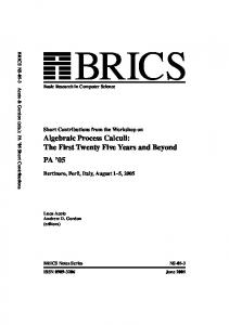
In this section we present a model of gene transfer by plasmid co-transfection1 involving non-Markovian reactions, derived from [23]. We model complex formation for green and red plasmids, together with the main stages of co-transfection (Fig. 1). The process C(g, r) represents a complex of g green plasmids and r red plasmids, where g, r are numbers. A complex can grow in size by receiving the numbers g 0 , r0 on channel bind and adding these to g, r respectively. Alternatively, it can bind to another complex by sending the numbers g, r on channel bind. At any stage a complex C(g, r) can enter the cell, represented by an enter reaction to DC(g, r). In this model, the rate of entry is proportional to the square of the size of the complex, where the size is given by the total number of red and green plasmids (g + r). The rate of entry relates to the charge of the molecule, where larger complexes have increased charge and are better able to penetrate the cell wall. Once translocation has occurred, the resulting complex of plasmids EN C can dissociate into individual green (EN G) or red (EN R) plasmids, one at a time. We model this using an unbind reaction, which removes a red or green plasmid from the complex. The unbinding rate is proportional to the number of red or green plasmids, respectively. The gene expression of plasmids involves the transcription of plasmids into mRNA and the transla1 Model and prototype simulator http://research.microsoft.com/spim

available

from

Figure 2: Simulation results of the plasmid cotransfection model of Fig. 1, where the horizontal axis represents time in hours and the vertical axis represents numbers of molecules.

Figure 1: A stochastic pi-calculus model of plasmid co-transfection.

tion of mRNA into proteins. The degradation of mRNA is a 170-step process which we model as a single reaction with an Erlang distribution. The green plasmids produce green fluorescent proteins (GFP ), while the red plasmids produce red fluorescent proteins (RFP ). The SPiM code for the model is given in Appendix A. Fig. 2 shows the results of simulating the model of Fig. 1, using the generic abstract machine instantiated with the non-Markovian stochastic pi-calculus. The model parameters are given in Appendix A. The individual plasmids stochastically bind together to form complexes of different sizes, which then enter the cell and move towards the nucleus. Entire complexes can be degraded while in transit. Once they reach the nucleus the complexes unbind, releasing their plasmid cargo, which is then transcribed to produce red or green

Figure 3: Simulation of the initial entry of complexes into the cell. We simulated the initial stages of the model of Fig. 1, starting with 1000 individual red and green plasmids and allowing these plasmids to form complexes before entering the cell. We let DC(g,r) = () to prevent further movement of the complexes and plot the composition of plasmids DC(g,r) immediately after entry. We used a 3D plot where the x axis represents the number of green plasmids in the complex, the y-axis represents the number of red plasmids in the complex and the height represents the number of complexes with the given composition of red and green plasmids. The largest complex contained 11 red and 9 green plasmids, but the majority of complexes contained less than 10 plasmids.

fluorescent proteins. In order to visualise the proportion of complexes of different sizes, we can plot the complexes immediately after entry into the cell (Fig. 3). In general the complexes can be of arbitrary size, depending on the initial populations of plasmids. Control over the ratio between transfected plasmids is a key requirement for the development of novel therapeutic strategies that act in the tissue on the gene level. Here stochasticity plays an important role. Future analysis of the model can be used as a basis for determining optimal co-transfection strategies that result in specific ratios of red and green fluorescent proteins inside individual cells.

6.

DISCUSSION

We have introduced a generic abstract machine for the simulation of process calculi with potentially unbounded numbers of species and reactions. Instantiating the machine for a particular calculus requires the definition of functions to extract the species and reactions from the processes of the calculus. We have detailed the simulation of the non-Markovian stochastic pi-calculus using this abstract machine, and have presented a model of plasmid co-transfection that illustrates the flexibility of the proposed framework. To cope with a large number of reactions when simulating non-Markovian processes with a large number of species, the implementation of the generic abstract machine should use optimised data structures to quickly access reactions affected by propensity changes. This requires either computing an explicit dependency graph between reactions, as suggested in [6], or having efficient hashing structures to access reactions in the machine term. For the Markovian case, we have characterised the improvement in simulation efficiency by the ability to count complexes that share private channels as a single species. More practical comparisons such as benchmark comparisons with existing stochastic pi-calculus simulators are left for future work. Little work has so far been done to provide efficient nonMarkovian simulations. In [1], the Gillespie algorithm is extended to delayed reactions, allowing non-Markovian simulation of these types of reactions. In the scope of process calculi, Priami has formalised the semantics of the stochastic pi-calculus models with general distributions [17]. The simulation proposed in [17] is based on automatic rescaling of the general distribution functions of transitions during the execution, in order to reflect the history of the execution, as needed for non-Markovian reactions. This strategy has been adopted and implemented to allow non-Markovian simulation of BlenX models [10, 16]. While rescaling distribution functions is manageable for distributions like Gamma or Hyper-exponential, more general distributions may be harder to compute. The non-Markovian simulation algorithm we propose does not rely on such a rescaling of distribution functions and therefore provides an efficient and straightforward simulation of reactions with arbitrary probability distributions. The algorithm relies on the fact that our generic abstract machine allows a potentially unbounded number of new species to be dynamically generated. Our generic abstract machine aims at simulating a broad range of process calculi. This range includes process calculi capable of n-ary reactions, and reactions having arbitrary stoichiometric coefficients. To highlight the flexibility of our approach, we have used our machine to simulate a

variant of the DSD calculus [14]2 . As a proof-of-principle, we have also instantiated the generic abstract machine to a variant of the stochastic bioambient calculus [12]. Since this calculus relates processes that may move between different ambients, it was necessary to extend the encoding of species to correctly translate interactions as “flat” reactions. This instantiation required the addition of a species renaming operator in the generic abstract machine, and is detailed in Appendix B. Although the instantiation can be significantly improved through further optimisations, this nevertheless produces the first simulation algorithm for a non-Markovian stochastic bioambient calculus. Further refinements to the algorithm are left for future work. Our approach can potentially be used to simulate a range of existing process calculi within the same framework. In future, this could allow models to be constructed from components written in different domain-specific languages, allowing exact stochastic simulation of heterogeneous systems. Our approach could also aid the development of future programming languages and calculi, by reducing the overhead for implementing custom stochastic simulation algorithms. Acknowledgements. Thanks to Filippo Polo for development of the SPiM user interface and visualisations.

7.

REFERENCES

[1] D. Bratsun, D. Volfson, L. S. Tsimring, and J. Hasty. Delay-induced stochastic oscillations in gene regulation. Proceedings of the National Academy of Sciences of the United States of America, 102(41):14593–14598, 2005. [2] F. Ciocchetta and J. Hillston. Bio-PEPA: A framework for the modelling and analysis of biological systems. Theoretical Computer Science, 410(33-34):3065 – 3084, 2009. [3] V. Danos, J. Feret, W. Fontana, R. Harmer, and J. Krivine. CONCUR 2007 - Concurrency Theory, chapter Rule-Based Modelling of Cellular Signalling, pages 17–41. 2007. [4] L. Dematt´e, C. Priami, and A. Romanel. Modelling and simulation of biological processes in BlenX. SIGMETRICS Performance Evaluation Review, 35(4):32–39, 2008. [5] R. Ewald, J. Himmelspach, M. Jeschke, S. Leye, and A. M. Uhrmacher. Flexible experimentation in the modeling and simulation framework JAMES II – implications for computational systems biology. Brief Bioinform, Jan 2010. [6] M. A. Gibson and J. Bruck. Efficient exact stochastic simulation of chemical systems with many species and many channels. The Journal of Physical Chemistry A, 104(9):1876–1889, 2000. [7] D. T. Gillespie. Exact stochastic simulation of coupled chemical reactions. J. Phys. Chem., 81(25):2340–2361, 1977. [8] D. T. Gillespie. Approximate accelerated stochastic simulation of chemically reacting systems. J. Chem. Phys., 115:1716–1733, 2001. [9] P. Lecca and C. Priami. Cell cycle control in eukaryotes: a BioSPI model. In BioConcur’03. ENTCS, 2003. 2

Simulator available at http://research.microsoft.com/dna

[10] I. Mura, D. Prandi, C. Priami, and A. Romanel. Exploiting non-Markovian Bio-Processes. Electr. Notes Theor. Comput. Sci., 253(3):83–98, 2009. [11] M. Pedersen and G. Plotkin. A language for biochemical systems. In Computational Methods in Systems Biology, volume 5307 of LNCS, pages 63–82. Springer, 2008. [12] A. Phillips. An abstract machine for the stochastic bioambient calculus. Electronic Notes in Theoretical Computer Science, 227:143–159, January 2009. [13] A. Phillips and L. Cardelli. Efficient, correct simulation of biological processes in the stochastic pi-calculus. In Computational Methods in Systems Biology, volume 4695 of LNCS, pages 184–199. Springer, September 2007. [14] A. Phillips and L. Cardelli. A programming language for composable DNA circuits. Journal of the Royal Society Interface, 6(S4):419–436, August 2009. [15] A. Phillips, L. Cardelli, and G. Castagna. A graphical representation for biological processes in the stochastic pi-calculus. Transactions in Computational Systems Biology, 4230:123–152, November 2006. [16] D. Prandi, C. Priami, and A. Romanel. Simulation of Non-Markovian Processes in BlenX. Technical Report TR-11-2008, The Microsoft Research - University of Trento Centre for Computational and Systems Biology, 2008. [17] C. Priami. Stochastic π-calculus with general distributions. In Proc. of the 4th Workshop on Process Algebras and Performance Modelling, CLUT, pages 41–57, 1996. [18] C. Priami, A. Regev, E. Shapiro, and W. Silverman. Application of a stochastic name-passing calculus to representation and simulation of molecular processes. Information Processing Letters, 80:25–31, 2001. [19] A. Regev, E. M. Panina, W. Silverman, L. Cardelli, and E. Y. Shapiro. Bioambients: an abstraction for biological compartments. Theor. Comput. Sci., 325(1):141–167, 2004. [20] A. Regev, W. Silverman, and E. Shapiro. Representation and simulation of biochemical processes using the pi-calculus process algebra. In Pacific Symposium on Biocomputing, volume 6, pages 459–470, Singapore, 2001. World Scientific Press. [21] D. Sangiorgi and D. Walker. The π-calculus: a Theory of Mobile Processes. Cambridge University Press, 2001. [22] T. Tian and K. Burrage. Binomial leap methods for simulating stochastic chemical kinetics. J. Chem. Phys., 121:10356–10364, 2004. [23] C. M. Varga, K. Hong, and D. A. Lauffenburger. Quantitative analysis of synthetic gene delivery vector design properties. Mol Ther, 4(5):438–446, Nov 2001.

APPENDIX A. SPIM CODE FOR PLASMID CO-TRANSFECTION directive sample 4.0 1000 val enter = 0.1 val degrade = 0.01

val val val val

detach = 1.0 transport = 1.0 translocate = 1.0 unbind = 1.0

val val val val

transcribe = 4.0 translate = 1.5 d_RNA = 0.466 d_protein = 0.019

new [email protected]:chan(float,float) new [email protected]:chan new [email protected]:chan let C(g:float,r:float) = do delay@enter*(g+r)*(g+r); DC(g,r) or !bind(g,r) or ?bind(g’,r’); C(g+g’,r+r’) or delay@degrade and DC(g:float,r:float) = do !attach; MDP(g,r) or delay@degrade and ENC(g:float,r:float) = do delay@degrade or delay@unbind*g; (ENG() | ENC(g-1.0,r)) or delay@unbind*r; (ENR() | ENC(g,r-1.0)) and MDP(g:float,r:float) = do delay@detach; DC(g,r) or delay@transport; PC(g,r) or delay@degrade; () and PC(g:float,r:float) = do delay@translocate; ENC(g,r) or delay@degrade; () and Microtubule() = ?attach; Microtubule() and ENG() = delay@transcribe; (ENG() | mRNAG()) and ENR() = delay@transcribe; (ENR() | mRNAR()) and mRNAG() = do delay@translate; (mRNAG() | GFP()) or delay@Erlang(170,d_RNA) and GFP() = delay@d_protein and mRNAR() = do delay@translate; (mRNAR() | RFP()) or delay@Erlang(170,d_RNA) and RFP() = delay@d_protein run 100 of C(1.0,0.0) run 100 of C(0.0,1.0) run 100 of Microtubule()

B.

SIMULATION OF THE STOCHASTIC BIOAMBIENT CALCULUS

The bioambient calculus was first presented in [19] for modelling mobile compartments in biological processes. This appendix describes how the bioambient calculus can be simulated using the generic abstract machine presented in the main text. Non-Markovian simulation can be achieved by means of Definition 3, producing the first non-Markovian simulation algorithm for the stochastic bioambient calculus.

B.1

Syntax and Reduction

The syntax and reduction rules of the stochastic bioambient calculus used in this section are presented in Definition 14 and are reproduced from [12]. A process P can be a choice of actions M , an instance X(˜ n) of a definition X with parameters n ˜ , a parallel composition of processes P | Q, a process νx P with a private channel x, or an ambient P consisting of a process P inside a compartment. A choice M

P, Q ::=

M | X(˜ n) | P |Q | νx P | P

Process

π1 .P1 + . . . + πN .PN

Choice

M ::=

E ::= X1 (m ˜ 1 ) 7→ P1 , . . . , XN (m ˜ N ) 7→ PN

Environnment τr .P + M

π ::= |

τr γ!x(˜ n)

0 local!x(˜ n).P + M | local?x(m).P ˜ + M0

Delay Send

0 Q | c2p!x(˜ n).P + M | Q0 | c2p?x(m).P ˜ + M0

r

−→ P Fx

−→ P | P 0 {m:=˜ ˜ n} F

x −→

| γ?x(m) ˜ | µ!x

Receive Move

|

µ?x

Accept

0 Q | s2s!x(˜ n).P + M | Q0 | s2s?x(m).P ˜ + M0

x −→

local s2s

Local Sibling

Q | in!x.P + M | Q0 | in?x.P 0 + M 0

x −→

| |

c2p p2c

Parent Child

Q | out!x.P + M | Q0 | out?x.P 0 + M 0

x −→

µ ::= |

in out

Enter Leave

Q | merge!x.P + M | Q0 | merge?x.P 0 + M 0

x −→

merge

Merge

γ ::= |

|

F

0 Q | p2c!x(˜ n).P + M | Q0 | p2c?x(m).P ˜ + M0

r

P −→ P 0

⇒

Q | P | Q0 | P 0 {m:=˜ ˜ n}

x −→ Q | P | Q0 | P 0 {m:=˜ ˜ n}

F

F

Q | P | Q0 | P 0

F

Q | P | Q0 | P 0

F

Q | P | Q0 | P 0

r

−→

P

Q | P | Q0 | P 0 {m:=˜ ˜ n}

P0

Definition 14. Syntax and core reduction rules of the stochastic bioambient calculus, based on [12]. Γ ::=

a, b Γ

I ::= X(˜ n) M V ::= ∅ | {Γ := Γ0 } is local (Γ1 , Γ2 )

, ∅

Location

species(0)

Species Renaming

species(P ) , species(P, (root1 , root2 )) species( P , (a, b)) , species(P, (a0 , a)) if fresh(a0 ) species(X(˜ n), Γ) , X(˜ n)Γ if E(X(˜ n)) = C

, Γ1 = Γ2

is sibling((a1 , b1 ), (a2 , b2 )) , a1 6= a2 ∧ b1 = b2 is child ((a1 , b1 ), (a2 , b2 )) , b1 = a2

species(X(˜ n), Γ) , species(P, Γ) if E(X(˜ n)) = P 6= C species(νx P, Γ) , species(P {x:=y} , Γ) if fresh(y) species(P1 | P2 , Γ) , species(P1 , Γ) ] species(P2 , Γ)

Definition 15. Assigning locations to species, where a, b represent globally unique ambient identifiers.

(S, R)#∅

, (S, R) ˜ V , (S, R#M V )#M

(S, R)#M V

, {(J#M V, F, M V 0 #M V, J 0 #M V ) | (J, F, M V 0 , J 0 ) ∈ R ∧ releq(J, J#M V )}

R#M V ˜ V ({S, (I → 7 (i, C))}, R)#M

, (S 0 , (I 0 , S 0 ) ⊕ R0 ) if I 0 = I#M V and S 0 = S 00 {I 0 7→ (i + i0 , C)} and ( if I 0 ∈ dom(S) then S(I 0 ) = (i0 , C) else i0 = 0) ˜ V and (S 00 , R0 ) = (S, R)#M Γ0

Γ0

releq({P1Γ1 , P2Γ2 }, {P1 1 , P2 2 }) , is local (Γ1 , Γ2 ) ∧ is local (Γ01 , Γ02 ) ∨ is sibling(Γ1 , Γ2 ) ∧ is sibling(Γ01 , Γ02 ) is child (Γ1 , Γ2 ) ∧ is child (Γ01 , Γ02 ) is child (Γ2 , Γ1 ) ∧ is

child (Γ02 , Γ01 )

∨ ∨

{Γ1 := Γ2 }#M V X(˜ n)Γ #M V

, {Γ1 #M V := Γ2 #M V } , X(˜ n)Γ#M V

Γ#{Γold := Γnew } , Γnew if Γ = Γold (c, d)#{a, b := a0 , b0 } , c, a0 if d = a and b0 = b Γ#{Γold := Γnew } , Γ otherwise.

Definition 16. Instantiation of the generic abstract machine to the stochastic biolambient calculus.

consists of a competition between zero or more actions π.P , where π is the action that can be performed, after which process P is executed. An action π can be a delay τr , a send γ!x(˜ n) of values n ˜ on channel x, or a receive γ?x(m) ˜ of values m ˜ on channel x, where γ denotes the type of communication. This can be inside the same ambient (local), from one sibling ambient to another (s2s), from a child ambient to its parent (c2p) or from a parent ambient to a child (p2c). In addition, an action π can be a move µ!x on channel x or an accept µ?x on channel x, where µ denotes the type of movement. This can be an ambient entering one of its siblings (in), a child ambient leaving its parent (out) or a merge of two sibling ambients (merge).

B.2

actions(X(˜ n)Γ ) , C {m:=˜ ˜ ˜ n} if C = E(X(m)) reactions(I, J) , unary(I) ] binary(I, J) unary(I) , {({I}, F, f, J) | (F, M V, J) ∈ delays(I) ∧ f (T ) = T #M V } delays(I) , {(Fr , ∅, species(P, Γ)) | τr .P ∈ actions(I)} if I = X(˜ n)Γ binary(I1 , J) , {({I1 , I2 }, F, f, J) | C2 = actions(I2 ) ∧ C1 = actions(I1 ) ∧ I1 = X1 (˜ n)Γ1 ∧ I2 = X2 (m) ˜ Γ2 ∧ I2 ∈ {I1 } ∪ J ∧ f (T ) = T #M V

Extracting Reactions from Ambients

The main challenge when instantiating the generic abstract machine with the bioambient calculus is to extract a “flat” set of reactions from a bioambient process. To achieve this, processes are labelled with the location in which they evolve. The location is a pair consisting of the identifier of the ambient in which the process is located, together with the identifier of the parent ambient. For instance, in the process

P1 | P2

, P2 has location (a, b), where a is the

identifier the ambient containing P2 and b is the identifier of the parent ambient. Both a and b denote ambient identifiers that are assumed to be globally unique. The assigning of locations to species is presented in Definition 15. The identifiers root1 and root2 denote the top-level enclosing ambient and the top-level parent ambient, respectively. When computing reactions, the process locations are used to check if processes are able to interact. The computation of reactions from a bioambient process is given in Definition 17 and relies on the predicates is local , is sibling and is child . For example, executing an s2s interaction between two species P1a1 ,b1 and P2a2 ,b2 requires that their parent ambients are equal but that their enclosing ambients are different, i.e. b1 = b2 and a1 6= a2 . When an ambient moves (by using in, out, merge actions), we relabel the species to reflect the change in location. As an example, consider the following reduction: Q1 | in!x.P1 | Q2 | in?x.P2

−→

Q1 | P1 | Q2 | P2

Rewriting this using process locations gives the reduction below: F

x b,c b,c −→ Qa,b | P1a,b | Qb,c Qa,c | in!x.P1a,c | Qb,c 1 2 | P2 1 2 | in?x.P2

and we obtain the corresponding reaction:

∧ (F, M V, J) ∈ interact(C1Γ1 , C2Γ2 )} interact(C1Γ1 , C2Γ2 ) , comm(C1Γ1 , C2Γ2 ) ] comm(C2Γ2 , C1Γ1 ) ] moves(C1Γ1 , C2Γ2 ) ] moves(C2Γ2 , C1Γ1 ) comm(C1Γ1 , C2Γ2 )

, {(Fx , ∅, J) | J = species(P1 , Γ1 ) ]species(P2{m:=˜ ˜ n} , Γ2 )) ∧ γ!x(˜ n).P1 ∈ C1 ∧ γ?x(m).P ˜ 2 ∈ C2 ∧ γ ∈ comm actions(Γ1 , Γ2 )}

}, J) moves(C1Γ1 , C2Γ2 ) , {(Fx , {Γ1 := Γnew 1 | J = species(P1 , Γ1 ) ] species(P2 , Γ2 )) ∧ µ!x(˜ n).P1 ∈ C1 ∧ µ?x(m).P ˜ 2 ∈ C2 new ∧ Γ1 = move path(µ, Γ1 , Γ2 ) ∧ µ ∈ move actions(Γ1 , Γ2 )} local ∈ comm actions(Γ1 , Γ2 ) ⇔ is local (Γ1 , Γ2 ) s2s ∈ comm actions(Γ1 , Γ2 ) ⇔ is sibling(Γ1 , Γ2 ) c2p ∈ comm actions(Γ1 , Γ2 ) ⇔ is child (Γ1 , Γ2 ) p2c ∈ comm actions(Γ1 , Γ2 ) ⇔ is child (Γ2 , Γ1 ) in ∈ move actions(Γ1 , Γ2 ) ⇔ is sibling(Γ1 , Γ2 ) out ∈ move actions(Γ1 , Γ2 ) ⇔ is child (Γ1 , Γ2 ) merge ∈ move actions(Γ1 , Γ2 ) ⇔ is sibling(Γ1 , Γ2 ) move path(in, (a, c), (b, c))

,

a, b

move path(out, (a, b), (b, c))

,

a, c

move path(merge, Γ1 , Γ2 )

,

Γ2

Definition 17. Instantiation of the generic machine to the Bioambient calculus. We assume a fixed global environment E that contains the species definitions. Note that we set f to be the species renaming function f (T ) = T #M V .

in!x.P1a,c + in?x.P2b,c −→ P1a,b + P2b,c As the ambient containing P1 and Q1 moves, the locations of P1 and Q1 have to be updated. This is specified by attaching to each reaction O the required location renaming (in the above example, the renaming is {(a, c) := (a, b)}). The renaming operation and the reduction relation obtained are presented in Definition 16. During the renaming of current reactions (R#M V ), we must check whether the change in location invalidates any existing reactions. This is achieved using the releq predicate presented in Definition 16. If the change in location means that species are too far apart to interact, the corresponding reaction is removed. As dis-

cussed in the main text, there is broad scope for calculusspecific optimisations. For example, unused reactions can be garbage-collected, ambients with the same contents can be grouped together as a single species, and complexes in the bioambient calculus can be treated in a similar fashion to complexes in the stochastic pi-calculus. The renaming function can also be optimised by using a hash table to directly access reactions concerned by the renaming. Finally, the proof of correctness of the abstract machine is left for future work.