AbstractâA new method, called genetic programming-spectral vegetation index (GP-SVI), for the .... 1http://www.spotimage.fr/html/_167_194_201_640_.php ..... transmission mechanisms, is at the core of the genetic process.4. As shown in Fig ...
2446
IEEE TRANSACTIONS ON GEOSCIENCE AND REMOTE SENSING, VOL. 46, NO. 8, AUGUST 2008
A Genetic-Programming-Based Method for Hyperspectral Data Information Extraction: Agricultural Applications Clément Chion, Jacques-André Landry, and Luis Da Costa
Abstract—A new method, called genetic programming-spectral vegetation index (GP-SVI), for the extraction of information from hyperspectral data is presented. This method is introduced in the context of precision farming. GP-SVI derives a regression model describing a specific crop biophysical variable from hyperspectral images (verified with in situ observations). GP-SVI performed better than other methods [multiple regression, tree-based modeling, and genetic algorithm-partial least squares (GA-PLS)] on the task of correlating canopy nitrogen content in a cornfield with pixel reflectance. It is also shown that the band selection performed by GP-SVI is comparable with the selection performed by GA-PLS, a method that is specifically designed to deal with hyperspectral data. Index Terms—Compact Airborne Spectrographic Imager (CASI) sensor, crop nitrogen, feature selection, genetic programming (GP), hyperspectral remote sensing, precision farming, site-specific management, spectral vegetation indices (SVIs).
I. I NTRODUCTION AND B ACKGROUND A. Context
R
ECENT development of hyperspectral imagery has brought a new challenge for information extraction techniques. Large amounts of data are now available for landscape studies (see [1] for example) or agricultural monitoring (e.g., [2] and [3]). For the latter, democratization of hyperspectral technologies of acquisition gave rise to great hopes for the assessment of crops’ biophysical variables throughout the growing season [4]–[6]. Knowledge obtained from the evaluation of these variables, coupled with variable-rate technologies (VRTs) (see [7] for details on VRTs), allows the farmer to undertake a site-specific management strategy; the net results include lower operating costs and reduced soil and water pollution due to chemical excess [8]. The early detection of stresses within crops is a critical step in precision farming; hyperspectral technologies give the opportunity to provide exhaustive, fastcollected, and relatively low-cost information from a whole field [9]. The aim of this paper is to derive an algorithm that can extract an adequate descriptive model for a continuous variable within a scene, given a hyperspectral data set and a set of in situ measures of this variable.
Manuscript received October 23, 2006; revised May 7, 2007. C. Chion and J.-A. Landry are with the École de Technologie Supérieure, University of Québec, Montreal, QC H3C 1K3, Canada. L. Da Costa is with the TAO Team, INRIA Futurs, 78153 Paris, France. Color versions of one or more of the figures in this paper are available online at http://ieeexplore.ieee.org. Digital Object Identifier 10.1109/TGRS.2008.922061
B. Problematic In many agricultural applications, the ability to assess a biophysical variable over a whole culture is key to improving its management. For example, the knowledge of canopy nitrogen variability in a field can help a farmer modulate his fertilizer supplies. If successfully conducted, this approach, called precision farming, yields ecological benefits with sustainable management of arable soils and also considerable economical savings for the farmer.1 The “ground truth” (knowledge acquired in situ about a geographical region) is essential in agriculture. This knowledge is key when studying hyperspectral data, and it is a great starting point when building descriptive models using interpolation or regression methods. One drawback is that ground truth data is often difficult and expensive to collect [10], particularly for agricultural applications (e.g., field campaigns and/or laboratory analyses). However, given that weather conditions [11], sensor types [12], correction steps, or noise can make remote sensing products less reliable [13], it is not yet possible to derive accurate “universal models” describing a scene variable that would be true in all configurations (i.e., accurate from one data set to another). These reference data are essential to perform any supervised machine learning (ML) strategy dealing with high-dimensional hyperspectral data. Informative about health status, quantitative relations between optical properties (mainly reflectance) and vegetation composition (e.g., pigment content, internal structure, or water content) are well established at the leaf level [14], [15]. However, when considering the canopy scale with remote sensing techniques such as satellite or airborne imagery, many factors prevent a simple basic extension of knowledge from leaf to canopy scales; Jacquemoud [16] identifies three types of distorting factors: external (incident radiance, measurement geometry, and atmosphere influence), internal (contribution of fruits, flowers, and stems in the reflectance; influence of canopy architecture, spatial distribution, and inclination of leaves; and density), and factors related to soil (mainly roughness and chemical composition). The latter will be of great importance for canopy zones characterized by low leaf area index (LAI), which is a dimensionless canopy physical variable representing the relative coverage of the foliage with respect to the underlying soil area. Intrapixel heterogeneity induced by sensor resolution is also a disturbing factor. Consequently, methods are required to minimize undesirable effects inherent to this type of 1 http://www.spotimage.fr/html/_167_194_201_640_.php
0196-2892/$25.00 © 2008 IEEE
CHION et al.: GP-BASED METHOD FOR HYPERSPECTRAL INFORMATION EXTRACTION
data and to extract a footprint of the biophysical variable under observation. Some approaches are discussed in the next section in order to set the context of hyperspectral data analysis. In Section III, data used in this paper and all associated processing steps are briefly described. In the second part, the genetic programming (GP) framework is presented, and the specificities of the GP-spectral vegetation index (SVI) algorithm are discussed. In Section IV, we present the strategy of the experiments to achieve our goals. Results and discussion are presented in Section V, and a general conclusion is drawn in Section VI. II. T ECHNIQUES FOR H YPERSPECTRAL D ATA E XPLORATION : A S HORT I NSIGHT Over the last few years, several approaches have been developed to deal with hyperspectral data specificities. In agriculture, SVIs, band selection techniques, and regression and classification methods are widely used. First elaborated for multispectral data exploration, SVI can be defined by ratios like “simple ratio” (SR) given by SR =
NIR R
(1)
(where NIR and R represent the reflectances in the near-infrared and red portions of spectrum, respectively), as well as by more complex arithmetic nonlinear combinations of spectral bands such as MSAVI2 [17], [18] given in (2), obtained from multiband sensors � MSAVI2 = (NIR+1)−0.5 (2·NIR+1)2 −8·(NIR−R). (2) SR is commonly used to estimate the green biomass [15], whereas MSAVI2 aims at reducing the underlying soil effect on canopy reflectance. In the realm of agricultural applications, SVIs have been widely investigated to model variations of diverse biophysical variables within fields. The classical approach to design SVIs consists of studying the reflectance curve of a piece of vegetation to find the spectral signature of the element under investigation by identifying relevant wavelengths (mainly peaks, gaps, and slopes). Once these particular wavelengths are found, arithmetic combinations are computed to extract effects of the variable observed from the rest of the information (e.g., see the transformed vegetation index [19]). However, this approach is limited to coarse singularities and leads to the loss of potentially relevant information contained in the rest of the broad reflectance spectrum [20]. Consequently, results obtained with this procedure are not always satisfactory, which has led some authors to develop new approaches to design SVIs. The most widely used SVI is certainly the normalized difference vegetation index (NDVI) which appears in many studies to describe diverse phenomena [21]–[23]; its main usage is to evaluate chlorophyll density in order to differentiate vegetation landscape from urban zones or water areas. Estimating nitrogen content over a wheat field, Hansen and Schjoerring [23] looked for the best pair of spectral bands (b1, b2) by following the general form of NDVI [defined by equation (3)] and considering the partial least squares (PLS) regression with ground measures NDVI =
b1 − b2 . b1 + b2
(3)
2447
The approach of Hansen et al. gave good results and confirmed that it is still difficult to proceed without “ground truth” for precise information extraction from remotely sensed data. Variations in reflectance associated with plant constituents’ variability (such as nitrogen content) within hyperspectral data are probably too subtle to overcome noise effects and inaccuracy resulting from the various image correction steps (radiometric, atmospheric, and geometric). Band selection techniques are a particular form of feature selection in ML [24]. Band selection aims at reducing the high dimensionality of hyperspectral data (frequently more than 100) by selecting only a subset of the spectral bands containing the relevant information for a specific application, reducing the complexity of the analysis. Indeed, many of the spectral bands are highly correlated (particularly the adjacent ones) and contain redundant information. So far, mostly standard statistical methods have been used for this purpose: multiple regression (MR), PLS regression [23], discriminate analysis [25], wavelet-based classification [26], or clustering [27]. Using NDVIs, transformed soil-adjusted vegetation indices, and MR, Thenkabail et al. [5] identified a subset of only 12 spectral narrow bands (ranging from 350 to 1050 nm) that could potentially describe principal crop variables (LAI, plant height, grain yield, and wet biomass); a sensor with 12 narrow bands could, in fact, be built for such applications, considerably decreasing problem complexity. Feature extraction techniques such as generalized local discriminant bases [28] or segmented principal component transformation [29] are also worth mentioning as a means of reducing problem complexity. Most of these investigations have been conducted mainly for classification problems; it would be interesting to test these techniques in the context of regression problems. Furthermore, reducing search-space dimension avoids the curse of dimensionality [30], a phenomenon characterized by a decrease in solution accuracy when input characteristic vector dimension (number of spectral bands in the case of hyperspectral data) exceeds a threshold value. GP has already been used in hyperspectral data analysis for supervised classification problems by combining spectral bands [31], [32] and via the development of image-processing algorithms [33] to extract scene features. Ross et al. [31] propose a GP-based approach to evolve “mineral identifiers” aiming at detecting whether a specific material resides within a hyperspectral image pixel. In order to recognize each material, a specific classifier is evolved, which will provide a binary output (present or absent) when applied to a new pixel. Some a priori knowledge about materials present in the scene is necessary to train each classifier separately. Brumby et al. [33] evolved fixed-length chromosomes representing a suite of image-processing primitives to generate a binary image representing burned regions in a scene; however, considering the fixed-length representation of individuals, this method is closer to the genetic algorithm (GA) paradigm. Contrary to previous works [31]–[33], GP-SVI aims at describing a continuous variable by evolving a regression model, consequently providing a continuous field solution instead of a binary output over the whole area. The GP-SVI algorithm is inspired both by SVI and band selection methods in the sense that it searches for a descriptive regression model that uses only a subset of the spectral bands that are then arithmetically combined. The strategy to find the best SVI describing a crop
2448
IEEE TRANSACTIONS ON GEOSCIENCE AND REMOTE SENSING, VOL. 46, NO. 8, AUGUST 2008
Fig. 1. Experimental field-plot spatial layout. The three nitrogen treatments correspond to low nitrogen (N0 , N of 60 kg · ha−1 ), normal nitrogen (N1 , N of 120 kg · ha−1 ), and high nitrogen (N2 , N of 250 kg · ha−1 ). This layout derives from a two-factor split-plot completely randomized design with the following constraints. Each combination Ni Wj appears four times, Ni soil treatments are contiguously nested within Wj blocks because they are well controlled, whereas Wj treatment blocks are spaced because they are vaporized, with much more risks of dispersion.
biophysical variable is inspired by GP, explaining the name of the proposed algorithm. III. M ATERIALS AND M ETHODS A. Materials 1) Experimental Design and Layout: Data used to test and validate the proposed method were collected during an intensive field campaign supported by the GEOIDE Network of Excellence in 2000. Several hyperspectral images and ground measurements were collected throughout the growing season of a test cornfield (Zea mays) stretching from sowing to harvest, on a field located at the seed research farm in the Macdonald campus of McGill University, Sainte-Anne-de-Bellevue, QC, Canada. The experimental field (cf. Fig. 1) was split up into 48 20 × 20 m plots with different combinations of weed and nitrogen treatments (cf. the caption of Fig. 1 for more details on these treatments), resulting in a strong spatial heterogeneity. The soils at this experiment site are classified as Bearbrook and Sainte Rosalie clays (both belonging to the dark gray Gleysolic group); their colors extend from dark brown to grayish brown, with a granular structure. Corn was sown on May 30, 2000, with a 75-cm row spacing at a rate of 76 000 seeds · ha−1 . Herbicides were applied on June 26, 2000, and nitrogen fertilizer was added prior to sowing and again in the second week of July. For an exhaustive description of the experimental plan, readers are referred to [2]. 2) Data Description: During the growing season, three flights were made with a Compact Airborne Spectrographic Imager (CASI) sensor to acquire hyperspectral images at key stages of the plants’ life. Data acquired are composed of 72 spectral bands ranging from 409 to 947 nm with ∆λ = 7.47 nm at a 2-m pixel resolution. Due to the presence of noise, the last two channels in the near infrared were removed from the analysis, resulting in 70 useful bands. At the time of each image acquisition, observations on canopy and soil biophysical vari-
ables were collected within the field to allow for the analyses of relations between remote spectral data and ground truth. For the validation step of the new method presented in this paper, only chlorophyll meter soil and plant analysis development (SPAD) data and LAI data were available as ground truth reference; these data are briefly discussed in the next section. a) Ground truth data processing: In this paper, we focused on canopy nitrogen content at the beginning of the tasseling stage, with data being taken early in August. During this period, 88 observations of plant nitrogen content were exploitable for analysis, taking into account that two measurements were needed to evaluate this quantity. First, SPAD chlorophyll meter measures were transformed into plant nitrogen concentration values using Dwyer’s relation [34]. This relationship was chosen because it was particularly developed for corn at the tasseling stage and reused in that specific context [35]. Second, these nitrogen concentrations were weighted using the LAI value to obtain a final value that is proportional to the total nitrogen content in a pixel [36]. Initially, two LAI measures were collected inside each of the 48 plots, for a total of 96 samples. Due to human errors,2 only 93 measures were available. A 3 × 3 mean filter was applied to hyperspectral data, as described in the next section, introducing border lane (soil areas between plots) effects for some sampling points; consequently, five more data were removed, leaving a total of 88 ground truth data points for the present paper. The quantity of canopy nitrogen in a given pixel depends on the following two factors: 1) the surface density of leaves (“how many leaves”) in that pixel and 2) the nitrogen level contained in the resident leaves (“how much nitrogen by leaf”). In that sense, both LAI and leaf nitrogen content influence canopy nitrogen in a given field zone (consequently in a given pixel), which explains our strategy (similar to the one adopted by Strachan et al. [36]). b) CASI data processing: Data were preprocessed by the research team of John Miller at the Centre for Research in Earth and Space Science, York University, Toronto, ON, Canada. This preprocessing comprises atmospheric correction, radiometric calibration, and geometric corrections, which are mandatory operations prior to the creation of a geographically referenced database. These geographic data were imported into a geographic information system (GIS) software (PCI GEOMATICA V9.1.6). A geographically referenced database was then created to make data manipulations easier. Once the preprocessing stage was executed, a 3 × 3 mean filter was applied onto the images for two reasons: First, SPAD measures were collected in a 1-m radius around each flag, which implies a possible influence of neighbor pixels due to spatial resolution; second, accuracy of the geometric correction is about 0.5 pixel [2] (about 1 m because of the 2-m image resolution) if one considers the error arising from GPS for assessment of flags’ positions. Once all processing was performed, relevant data were extracted from the GIS environment to be treated using the GPSVI algorithm programmed using Microsoft Visual C++ V6.0. 2 The sources of errors for nitrogen assessment are not a major problem for this paper because our goal is not to advance new results in agronomy but to rather propose a new method that is able to extract descriptive models of crop biophysical variable.
CHION et al.: GP-BASED METHOD FOR HYPERSPECTRAL INFORMATION EXTRACTION
2449
composition of good descriptive models. However, there exists an overlap between classes (standard deviations are not plotted for clarity), implying that information in this domain is not sufficient to accurately describe nitrogen; this highlights the need to explore the rest of the spectrum. The succeeding section presents the GP-SVI method. First, a general description of GP is given, followed by the explanations of adjustments and choices made relative to the GP-SVI algorithm. B. Methods
Fig. 2. Spectral response of canopy at the 88 sample locations of the Macdonald farm, as measured by the CASI hyperspectral sensor early in August.
Fig. 3. Mean reflectance curves plotted for three nitrogen classes. It is obvious that the maximum variance lies in the near-infrared portion. In this region of the spectrum, reflectance is positively correlated with canopy nitrogen content (i.e., LAI and leaf nitrogen concentration).
CASI spectra at the 88 pixels (extracted at sample geographical locations) are shown in Fig. 2. The maximum variability among sample reflectance curves is located in the NIR part of the spectrum for wavelengths greater than 750 nm. We also noticed that, around the reflectance peak in the green portion (∼550 nm), data variance is relatively high. In an attempt to potentially locate discriminating portions of the spectrum region regarding canopy nitrogen, we split reflectance curves into three classes of low, medium, and high canopy nitrogen content and show the mean reflectance curve of each class in Fig. 3. It is noticeable that canopy nitrogen content and its reflectance in the near-infrared portion are positively correlated; keeping in mind that canopy nitrogen content in a pixel is influenced by both LAI and leaf nitrogen concentration (cf. Section III-A2a), this observed correlation is assumed to be due to LAI variability, which is known to influence NIR reflectance (see [37, p. 206]). Zooming in on the other portions of the reflectance spectrum does not offer anything similar. Because of these preliminary observations made on our data set, we expected to find spectral bands in this portion in the
1) GP: General Presentation: GP is part of the ML field and, in particular, a branch of evolutionary computation (EC) in artificial intelligence techniques. Koza [38] introduced GP in 1992, which is a derivation of the GA paradigm proposed by Holland [39], [40]. The main difference between GA and GP is that solutions in GA are (conventionally) fixed in length, whereas GP allows variable length solutions. Consequently, the shape of the solution is free in GP, whereas it is fixed initially in conventional GA. GP foundations come from the Darwinian theory of species evolution [41] in the sense that, among a “population” (i.e., a subset of “possible solutions”), there is selection of “individuals” well adapted to their “environment” (i.e., “potential solutions” giving a good answer to the “problem constraints”). During a process of reproduction, groups of two selected “individuals” will give a part of their “genome” (“structure”) to produce two “children” (i.e., new “potential solutions”) who will take place in a new “generation” (i.e., new subset of “possible solutions”). After selection for the reproduction process, several functions, called genetic operators or genetic functions, are applied with an associated probability. The two principals are the crossover and mutation operators that are inspired by genetic phenomena, associated with DNA, during sexual reproduction (cf. Figs. 4 and 5). In the following section, details on these operators will be presented in the context of GP-SVI. In several application fields, GP proved its efficiency, providing sometimes better results than solutions designed by humans. Computational molecular biology [42], cellular automata, sorting networks, analogical electrical circuits [43], controllers, and antennas are some of these fields, according to EC specialists.3 GP is particularly relevant in answering problems of different types, such as nonanalytical solvable, multiobjective, badly formulated, and complex problems or problems with a solution space of infinite dimension. However, an unavoidable preliminary step in the utilization of GP is to acquire a deep knowledge of the application field and the specific problem to solve. No “magic formula” exists, and adjustments and choices must be made regarding the specificities of the problem. This is discussed in the next section. 2) GP-SVI Algorithm: a) Algorithm overview: The aim of the method is to evolve, with the use of GP, a descriptive regression model linking ground truth observations (canopy nitrogen content in this paper) to an SVI. To this end, the GP-SVI algorithm explores the solution space composed of arithmetic combinations 3 http://www.genetic-programming.com
2450
IEEE TRANSACTIONS ON GEOSCIENCE AND REMOTE SENSING, VOL. 46, NO. 8, AUGUST 2008
Fig. 4. Classical crossover function applied between two binary trees. In this figure, bi is the value of the ith band of the CASI sensor as described before.
generation. The rest of the population is then filled by the repeated selection of pairs of individuals, their crossings, and their mutations. Crossover and mutation functions will then be processed between pairs of selected individuals, each one with an associated probability of occurrence. Crossover is considered as the core of GP [38], and consequently, its probability of occurrence is close to one. On the other hand, mutation is often a low-probability event introducing new material and creating diversity with the risk of destroying good solutions. Some of these parameter values were optimized through a sensitivity analysis presented in Section IV, whereas the others were chosen empirically. b) Representation: Binary trees: An individual is represented by a binary tree structure, which consists of nodes, each having a value, followed by two nodes (for nonterminal nodes) or none (for terminal nodes). In that way, each solution is defined by a (computational) tree. This structure is chosen for its simplicity of implementation and its ability to describe the entire solution space; indeed, the sought solution is an arithmetic combination of bands in order to build any type of arithmetic sequence. This structure is shown in Figs. 4 and 5 (description of genetic operators). We also need a reading convention to avoid ambiguity under noncommutative operator nodes (“/” and “−”); we choose to give the priority to the left branch of each node to settle this problem. Finally, a tree is read from the bottom to the top of the tree. Parent 1 in Fig. 4 would be read as (b53 − b35 )/(b53 + b35 ). c) Grammar and building rules: The sought solutions have the shape of an SVI, which implies that each individual is a more or less complex sequence of arithmetic operations between spectral bands. Consequently, using language theory formalism, we are able to propose the following context-free grammar G, which is defined as a quadruple G = (N, Σ, P, S) where N set of variables (nonterminal); Σ set of constants (terminal); P set of production rules; S start symbol with the following definitions: N = {O, B, S}
Fig. 5. Punctual mutation function applied on a binary tree.
of spectral bands, similar to SVI; it does so by evaluating the strength of the correlation between each of the potential solutions and ground truth observations. The first step is the creation of an initial population of potential solutions (i.e., arithmetic combination of spectral bands), according to simple rules defined later. Once the initial population has been created, for all population individuals, a score is assessed via a fitness function. The individuals are ranked according to this score, and the best of them (the “elite”) will proceed directly to the following
Σ = {oi , bj }, with 1 ≤ i ≤ 4 and S → O O → oi OO → oi BO P = → oi OB → oi BB B → bj
1 ≤ j ≤ 70
where oi set of arithmetic operators; oi = {‘+’, ‘−’, ‘÷’, ‘×’}; bj set of CASI spectral bands; bj = {b1 , b2 , . . . , b70 }.
CHION et al.: GP-BASED METHOD FOR HYPERSPECTRAL INFORMATION EXTRACTION
These basic rules allow the stochastic creation of an initial generation and provide the basis to build the children resulting from the application of genetic operators. Examples of randomly created individuals are shown in Figs. 4 and 5. We will later discuss additional building rules in Section IV-B. d) Fitness function and selection criteria: Once the first population is randomly built, one has to evaluate each individual’s ability to solve the problem. To do so, we must determine an objective with specific constraints if necessary. The relevance of a potential solution (SVI computed from hyperspectral data) was evaluated by calculating its correlation strength with ground truth data. To this end, we investigated four basic regression types: linear, exponential, logarithmic, and power. Pearson coefficients were stored for each individual in order to elaborate a selection strategy. Another factor is that the solution searched for has to be as general as possible; moreover, as code bloat (exponential increase of individual’s structure size with negligible improvements of fitness scores) is a threat in GP, we opted to give penalty to large individuals. This idea follows the Occam’s razor principle (see [44, p. 67]) which states that “other things being equal, simple theories are preferable to complex ones.” The strategies tested to this end are described below. Regression is computed between each individual and ground truth training data set. Retaining Pearson coefficient Rk , indicating the strength of the correlation, we built a fitness function penalizing length; in this case, the fitness value of each individual k is calculated using f (k) = �
|Rk | � �� . 1+Lk 1 + log 1+L min
(4)
Consequently, the probability P (k) for an individual k to be selected among the n-size population is given by f (k) P (k) = � . n f (i)
(5)
i=1
Length Lk is computed by summing the tree nodes forming an individual k (for example, Lk = 7 in Fig. 5); if Lk = Lmin , the fitness is reduced to the Pearson coefficient, and the probability P (k) is equivalent to classical wheel shown in (5). The logarithmic operator is introduced to smooth the length penalty; indeed, it was found that a simple normalization of Rk by length Lk was too selective, reducing the mean length of all population solutions to a little more than Lmin . Observing that a loss of diversity among the selected individuals leads to a drop in overall performances, we introduced a preliminary first-round tournament with a classical wheel selection. At the end of this first step, four different individuals are selected for the second round with the probability mentioned in (6), only considering Rk . Then, by calculating f (k) and P (k) for each individual, two of them are chosen for reproduction P (k) =
|Rk | , i=N � |Ri | i=1
where |Rk | = + Rk2 .
(6)
2451
In the following section, genetic operators are briefly discussed; as they represent the core of the GP process, they are revisited in the context of the GP-SVI method. e) Genetic functions: Crossover: The crossover operator, inspired by DNA transmission mechanisms, is at the core of the genetic process.4 As shown in Fig. 4 (in the case of binary tree structure representation chosen in this paper), this operator allows the exchange of two subtrees coming from two parents, selected based on their fitness, to engender two children. The associated probability of occurrence of the crossover function is chosen to be high (pc > 80%), in accordance with its dominant role in the evolutionary process. Although genetic-oriented strategies based on crossover are not mathematically proven to lead to global maximum convergence, probabilistically, they do because of the implicit parallel search [45]. However, one has to pay attention to specific problems with crossover; some authors believe that this operator is mainly responsible for “code bloat” (exponential increase of individuals’ size through iterations), inevitably leading to failure of the convergence. To avoid such a problem (or at least to delay its occurrence), some authors have proposed solutions [46], [47]. The strategy that we adopted is described in Section IV. Mutation: The role of the mutation operator is twofold: It introduces “new” elements during iterations, and it can rescue parts (subtrees) of solutions, preserving them from introns, as shown in Fig. 5. The role of the mutation operator is important in the GP process, and this is demonstrated later in the section devoted to the parameter selection. However, its probability of occurrence was chosen to be low (pm < 20%) to avoid the systematic “killing” of the good solutions at the output of crossover. Here, again, many other mutation operators have been developed, but it is beyond the scope of this paper to test them. Elitism: The elitism operator aims at preserving the best individuals between generations. The form of elitism used in this paper is called “strong” elitism in the sense that it systematically transfers (in a deterministic way) a fixed proportion pe of the best individuals from generation N to N + 1. The influence of pe is presented in the section devoted to the results. IV. S TRATEGY OF E XPERIMENTATIONS A. Benchmark Experiments presented later have two distinct goals. The first goal is to assess GP-SVI performances in terms of its potential to compute good descriptive models of a crop biophysical variable. These performances are compared with statistical methods: MR, PLS combined with GA (GA-PLS), and treebased modeling (TBM). Classical SVI performances are also computed, and the best one is reported. The second goal is to evaluate GP-SVI’s ability to perform band selection; we compare its results with those provided by GA-PLS [48], [49] (commonly used in chemometrics with spectral data).5 4 http://www.genetic-programming.com 5 An additional implicit objective is to confirm that GP has the potential to accurately extract information from hyperspectral imagery.
2452
IEEE TRANSACTIONS ON GEOSCIENCE AND REMOTE SENSING, VOL. 46, NO. 8, AUGUST 2008
All experiments are performed on the data sets described in Section III. MR will not be described, as it is a classical statistical method, but a brief overview of GA-PLS and TBM will be presented. The GA-PLS method was proposed by Leardi [48], [49] and is particularly useful in the case of spectral data. This method aims at making feature selection before performing PLS regression between a very large amount of descriptors (often spectral data) and a set of observations. This feature selection is performed using GA, and a complete description is given in [48]. To our knowledge, GA-PLS has not been used in remote sensing. Its comparison with GP-SVI is possible because of the availability of GA-PLS6 source code in MATLAB. The TBM algorithm selected is M5P [50], an improvement of Quinlan’s algorithm M5 [51]. M5P grows a tree-based model where each leaf is a regression model on the most discriminating attributes of the data. Consequently, this algorithm provides continuous piecewise models, unlike regression models where each leaf is a constant value. M5P is implemented within the Weka v.3.4 software [52]. To evaluate algorithms’ performances, we consider two indicators. The first is the explained variance R2 (in percentage) of model prediction against nonlearned ground truth data. The second is the relative generalization error rmse% , as defined in
� i=n �� � yi − yi )2 � i=1 (ˆ � rmse% = � i=n . (7) � (yi )2 i=1
Here, yˆi represents the nitrogen value estimated by the regression model, and yi is the in situ nitrogen measurement. In the next section, precautions taken to overcome GP pitfalls are presented. B. Special Precautions Three major flails threaten the successful course of GP in general and GP-SVI in particular. The first one arises when all individuals in a population become very similar, leading to the loss of diversity within a population. This poses the problem of precocious convergence of the solution and a failure in reaching a global maximum. The second flail, mentioned earlier, is known as “code bloat.” This phenomenon is characterized by an exponential increase of the individuals’ structure size with negligible improvements of fitness scores; this is apparently caused by the proliferation of introns (noncoding subparts in an individual’s structure) [53], although it is still much debated (see, for example, [54]). Finally, the last pitfall of GP is the phenomenon of “overfitting,” a structural problem of ML techniques, characterized by the increase in generalization error (assessed on a nonlearned data subset) coupled with a negligible improvement in performances on the learning data set. The three problems mentioned here are probably not independent, and strategies used in this paper to overcome them are described hereafter.
6 http://www.models.kvl.dk/intranet/dl-monitor/go.asp?get=genpls.zip
In order to solve these problems or, at least, to alleviate them, we adopted several additional rules. These strategies were kept and validated as they improved the overall results on our data set. The development of other effective strategies could be imagined and is the goal of numerous efforts in evolutionary algorithm (EA) research. 1) Removal of Doubloons: This first strategy is radical; all individuals in a new population are scanned in order to remove (suppress) copies of any individual. For any deleted solution, a new one is created with the same parameters as for building the first generation. This measure was taken in order to minimize the loss of diversity associated with the duplication of some good solutions. This resulted in a slower convergence but in more relevant best solutions. 2) Banning the “Consanguinity”: This rule forbids the selection of the same individual twice at the first and second rounds of the tournament. Intuitively, one can feel that sharing a subtree of a solution with itself does not promote the diversity and may lead to early convergence. 3) No “Monoband” Individuals: Considering that we want to promote diversity, it is clear that a solution composed of only one spectral band does not have more influence than a simple mutation. As the number of individuals present in any population during the process is constant, it is considered that “monoband” individuals just take the place of a potentially more interesting one, consequently reducing the diversity. In the grammar defined in Section III, this strategy is highlighted by the fact that the starting symbol S is constrained to be followed by O, representing the set of operators. This also implies that parameter Lmin = 3 in (4). 4) Maximal Length Parameter: To reduce code bloat, we chose to introduce a threshold length parameter that allows the elimination of solutions that are too long. This threshold value was chosen experimentally. 5) Maximal Depth for the First-Generation Individuals: We also introduced a parameter max _prof which limits the depth (number of tree levels) of randomly created individuals in the first population. We know that the size (number of nodes) of individuals tends to increase in an exponential manner, and instinctively, it implies that it is better to create simple (short) solutions at the outset, letting the evolutionary process increase the complexity of the individuals. Of course, this measure helps avoid early bloat by starting with simple individuals. This parameter will be optimized with a sensitivity analysis. 6) Length Penalty During the Selection Process: This measure, introduced earlier, tends to limit code bloat and indirectly helps to delay overfitting, as a long solution is more likely to be overtrained than a shorter one. In the next section, we present the GP-SVI parameter selection process.
C. Parameter Selection In order to avoid the overfitting phenomenon, we evaluated the generalization error through the process; this error tends to decrease rapidly at the outset and then slowly after a few iterations. Overfitting appears when the error on validation data set starts to increase again, and we stop the learning step when reaching the minimum validation error iteration.
CHION et al.: GP-BASED METHOD FOR HYPERSPECTRAL INFORMATION EXTRACTION
2453
TABLE I SIMULATION PARAMETERS
Fig. 6.
Sensitivity curves for pe parameter optimization.
Genetic strategies present another disadvantage in the great number of parameters that have to be optimized. Several optimization methods exist for the selection of parameters such as design of experiments [55], simulated annealing [56], or genetic algorithms. We chose to carry out a sensitivity analysis of the most influent parameters while empirically selecting the values of the remainders. Concerning the regression type, we noticed that, for every batch of simulations (the other parameters being fixed), logarithmic regression always gave appreciably better average results than linear, exponential, or power. Thus, we chose to use logarithmic regression for all experiments. The number of generations (Ng ) and the number of individuals (Nind ) are closely linked parameters, as their respective values are limited by computer performances and define the search endeavor. Ng is also chosen considering the occurrence of overfitting; for all runs, we observed that this problem never appeared before the 2850th iteration. We fixed Nind = 300 and Ng = 3000. As mentioned earlier, we introduced a parameter that kills an individual whose length exceeds a threshold value max _node. This value does not affect the fitness scores in the range of understandable SVI size, and we chose max _node = 25 as a compromise. Beyond this threshold value, we observed intron proliferation. Crossover probability pc does not have a great influence on fitness, except with using very low values. We chose a very high value of 98%, following a series of test observations. The three remaining parameters show greater influence on the process results and were optimized via a sensitivity analysis. First, Fig. 6 shows the sensitivity curves for the percentage of population selected by elitism (parameter pe in Table I). We obtained better performances with pe = 10%. Fig. 7 shows the sensitivity curves for the probability associated with the mutation operator (pm in Table I). The best performance was observed when pm = 10%. Fig. 8 shows the performance of the method when the maximum individual depth is varied (max _prof in Table I). This was chosen to be three. It is remarkable that, in the case of mutation and elitism, the lowest values always give the worst results, which confirms
Fig. 7. Sensitivity curves for pm parameter optimization.
Fig. 8. Sensitivity curves for max _prof parameter optimization.
that these two operators are essential for the parallel search. All parameter values and descriptions are summarized in Table I. General results are now presented and discussed.
2454
IEEE TRANSACTIONS ON GEOSCIENCE AND REMOTE SENSING, VOL. 46, NO. 8, AUGUST 2008
TABLE II COMPARED PERFORMANCES ON A TEST DATA SET
TABLE III TEN MOST OFTEN SELECTED BANDS IN THE BEST-RUN MODELS BY GP-SVI AND GA-PLS OVER 40 RUNS
V. R ESULTS AND D ISCUSSION We found two main results searching for a model that explains nitrogen distribution through a cornfield. First, GP-SVI improved the performances (on our data set) of all other tested methods, according to the two indicators mentioned. Models derived from regression between all classical SVI and nitrogen measures were tested, and the results from the best performance [named NDVIHANSEN , defined in (8)] are shown in Table II � �
i=51 i=42 � � 1 1 × b × b − i i 6 2 i=46 i=41 �
�. (8) NDVIHANSEN = i=51 i=42 � � 1 1 × b × b + i i 6 2 i=46
i=41
In order to perform an unbiased assessment of GP-SVI performances, we performed a k-fold cross-validation test with k = 11, which the ML community recommends in experiments with small data-set size [57]. The idea is to split the whole data set into 11 equally sized blocks of data: nine blocks used for training, one block used to assess rmse validation during the process, and the last block used to assess the generalization error reported in Table II. This procedure is repeated 11 times in order to validate and test GP-SVI using all blocks. Because of the small data-set size, this approach minimizes the risk that performance assessment will be biased by a specific configuration of the training data set. In order to be consistent for the 11 runs, each block was constituted with respect to the global distribution of nitrogen values in the whole data set; this procedure is called stratification. Note that k = 10 is a standard for this approach, but k = 11 was chosen to build k equally sized blocks (88/11 = 8). Although GP-SVI results in better performance on average, the variability through the runs is larger than that with GA-PLS (cf. Table II). This noticeable difference between performance variabilities comes from two factors. First, GA-PLS performs a feature selection before computing its best model search, which considerably reduces the variability in the set of the best models found through several runs. Second, GP-SVI considers as “best individual” the one that minimizes rmse on the validation subset up until iteration 3000. We, however, observed that, for some specific runs, better solutions appeared after iteration 3000. A different strategy could be to keep one of these fitter solutions; as in agricultural applications, we search for an ad hoc solution
to a given configuration (a specific biophysical variable such as nitrogen within a specific field) and do not pretend to find a universal SVI that is capable of describing a biophysical variable. TBM M5P performs well regarding rmse; however, explained variance (R2 ) fluctuates considerably between runs. This is interpreted as the consequence of outliers [58]. Indeed, these data distort the error calculation during tree growth, leading to an inaccurate model with poor generalization errors. Finally, MR with band selection offers lower performances than GP-SVI. During the learning step of GP-SVI, the pressure on individual selection is related to the maximization of |R| via the fitness function (4), which explains the adequate test performance regarding R2 . Moreover, this learning step is terminated when rmse is minimized on a validation set, which explains why GPSVI offers the best tradeoff in generalization, both on variance explanation (R2 ) and rmse minimization. The second analysis concerns band selection; GP-SVI results are quite close to those obtained by GA-PLS (Table III). These results were obtained by counting the ten most often selected spectral bands over a series of 40 runs. The percentages shown in Table III (second row on each method) represent the occurrence of each band in the best-run model for each method. From Table III, we observe that GP-SVI and GA-PLS have 40% of agreement on the most selected bands (b9 , b10 , b19 , and b31 ). Moreover, 20% of the other most selected bands are just one band apart. Values on percentage of occurrence are higher for GA-PLS, primarily because the number of distinct bands constituting the best-run model is 21 on average for GA-PLS and 10 for GP-SVI (because of constraint parameter max _node = 25). GP-SVI selected regions around 428 and 682 nm (ignored by GA-PLS); both methods chose reflectance at 550 nm. This is consistent with the work by Filella et al. [25] who identified reflectances at 430, 680, and 550 nm, discriminating wheat nitrogen status. We also noticed that b10 (480 nm) is widely the most selected CASI band over all runs for both GA-PLS and GP-SVI, indicating a clear possibility that the canopy’s absorption of light in the blue portion would be linked to its
CHION et al.: GP-BASED METHOD FOR HYPERSPECTRAL INFORMATION EXTRACTION
2455
VI. C ONCLUSION
Fig. 9. Good descriptive model defined by 10.843 × ln(IV1 ) − 19.987 represented as a grayscale image. White values correspond to high canopy nitrogen content, whereas black ones represent low nitrogen content. It is possible to note that, for each block of three-adjacent-Ni Wj treatment combination (cf. Fig. 1), it is always possible to identify N1 (the globally darkest), N2 , and N3 (the globally brightest) treatment.
level of nitrogen. This is interesting, as the interpretation of Fig. 3 (see Section III-B2) leads to the idea that the infrared domain could be relevant for canopy nitrogen quantification, but nothing pointed to the importance of band b10 . This highlights the limitation of visually selecting spectral bands by only observing reflectance curves. To illustrate the relevance and transparency of GP-SVI outputs, the best model of a GP-SVI run has been analyzed and is shown in Fig. 9. The mathematical expression of nitrogen model Npredicted given in (10) uses the SVI that is called IV1 b3 × b8 × (b10 ) × b56 b31 × (b37 )2 × b70 × (b34 −b63 + b47 ) 3
IV1 =
Npredicted = 10.843 × ln(IV1 )−19.987.
(9) (10)
We observe that three bands (b3 , b8 , and b10 ) are located in the blue part of the reflectance spectrum, four in the nearinfrared (b47 , b56 , b63 , and b70 ), two in the red portion (b34 and b37 ), and finally, one (b31 ) in the green part. A closer look at the bands selected reveals interesting patterns. Indeed, although NIR bands are the most numerous, the contribution of the ratio b56 /b70 is minor because it is almost constant throughout the data set (coefficient of variation of 2.5%). Band b47 belongs to the end of the red edge region (756 nm), known to be a good indicator of plant chlorophyll content [25], itself positively correlated with nitrogen [37]. Consequently, the presence of band b63 must be related to LAI because this physical crop parameter is calculated to compute the amount of nitrogen content in a pixel (cf. Section III-A2a). b63 is then the most influent spectral band in the NIR domain within IV1 . This short analysis of NIR bands in a solution generated by the GP-SVI solution provides an idea of the potential of this method to explore the whole spectral domain. Constraining the number of bands in a solution found via GP-SVI allowed us to find interpretable solutions which are consistent with knowledge found in the literature.
This paper presented an adaptation of GP, GP-SVI, for the extraction of information from hyperspectral data. The performance of the method was tested on a real application problem, so some real-world inherent limitations had to be dealt with, particularly concerning the lack of data (in situ agricultural data are human resource consuming and expensive to collect). Hyperspectral data contain large volumes of information, and extraction of the relevant part associated with a specific application is a great challenge. Statistical methods are often chosen for these types of problems, mainly because of their strong fundamental basis. EC approaches are less friendly than statistical techniques, specifically because of the great number of parameters to optimize and the threat of overfitting or code bloat (for GP). However, in the context of an agricultural application, we showed in this paper that improvements with the task of canopy nitrogen description were obtained by the GP-SVI method as compared to classical approaches. It is important to note that GP-SVI can be extended to any regression problem between a set of explicative variables and a set of observations in several fields (such as chemometrics or financial applications). We mentioned that the goal of this paper was not to advance new knowledge in agronomy because of noisy data, although the presented results appear to be in accordance with the literature. However, in a context of sitespecific management, we demonstrated that GP-SVI was able to overcome real-world data-related problems, such as data scarcity, to produce understandable solutions that outperform other regression methods. We would like to conclude this paper with the following three important points. 1) Techniques of images’ corrections (atmospheric, radiometric, and geometric) are constantly evolving; however, there are still major difficulties associated with the finding of “pure” indices describing biophysical variables. In other words, there is still a significant dependency on outer variables. Overcoming this difficulty is only possible through the intervention of the manual field worker, who will know where to look for ground truth representative of the field. This is usually not a problem for an agricultural producer who has a good knowledge of his field. The ability of generalization of our algorithm depends heavily on the quality of data used during learning. 2) An important issue with our algorithm is common to all metaheuristic optimization methods, such as EAs. These methods are usually evaluated, performing limited empirical studies where the algorithms’ parameters are hand tuned. This is due to many constraints, and the shortcomings of this methodology have already been elucidated [59]–[61]. However, the fact is that parameter settings may often have significant influence on the performance of EAs, and finding good parameter values can itself be a difficult optimization problem [62]. Ideally, we would like to be able to generalize our results for a large experimental space over the algorithm’s parameter values. A brute-force algorithm would be too expensive for this kind of task, and studying methods like the one proposed in [62] would be beneficial.
2456
IEEE TRANSACTIONS ON GEOSCIENCE AND REMOTE SENSING, VOL. 46, NO. 8, AUGUST 2008
3) Finally, concerning the repeatability of GP-SVI, we are confident that, using the present data set with parameters given in Table I, one will obtain models with performances as described in Table II. Due to stochastic processes involved in GP-SVI, model expression and SVI developed for each run would not be strictly identical; however, spectral bands retained will be consistent through runs with those presented in Table III. Moreover, contrary to problems where an exact solution exists or to problems with synthetic data sets, we addressed an application with a real-world data set, which is imperfect by nature. In this view, it would be wrong to pretend the best solution (if one exists) is reached with GP-SVI or any other EAs. ACKNOWLEDGMENT The authors would like to thank the National Sciences and Engineering Research of Canada for their financial support and the anonymous reviewers for their insightful comments and advice. R EFERENCES [1] G. P. Asner, C. A. Wessman, C. A. Bateson, and J. L. Privette, “Impact of tissue, canopy, and landscape factors on the hyperspectral reflectance variability of arid ecosystems,” Remote Sens. Environ., vol. 74, no. 1, pp. 69–84, Oct. 2000. [2] P. K. Goel, S. O. Prasher, J. A. Landry, R. M. Patel, R. B. Bonnel, A. A. Viau, and J. R. Miller, “Potential of airborne hyperspectral remote sensing to detect nitrogen deficiency and weed infestation in corn,” Comput. Electron. Agric., vol. 38, no. 2, pp. 99–124, Feb. 2003. [3] P. K. Goel, S. O. Prasher, R. M. Patel, J. A. Landry, R. B. Bonnell, and A. A. Viau, “Classification of hyperspectral data by decision trees and artificial neural networks to identify weed stress and nitrogen status of corn,” Comput. Electron. Agric., vol. 39, no. 2, pp. 67–93, May 2003. [4] D. Haboudane, J. R. Miller, E. Pattey, P. J. Zarco-Tejada, and I. B. Strachan, “Hyperspectral vegetation indices and novel algorithms for predicting green LAI of crop canopies: Modeling and validation in the context of precision agriculture,” Remote Sens. Environ., vol. 90, no. 3, pp. 337–352, Apr. 2004. [5] P. S. Thenkabail, R. B. Smith, and E. D. Pauw, “Hyperspectral vegetation indices and their relationships with agricultural crop characteristics,” Remote Sens. Environ., vol. 71, no. 2, pp. 158–182, Feb. 2000. [6] P. K. Goel, S. O. Prasher, J.-A. Landry, R. M. Patel, A. A. Viau, and J. R. Miller, “Estimation of crop biophysical parameters through airborne and field hyperspectral remote sensing,” Trans. ASAE, vol. 46, no. 4, pp. 1235–1246, 2003. [7] J. K. Schueller, “A review and integrating analysis of spatially-variable control of crop production,” Fertil. Res., vol. 33, no. 1, pp. 1–34, Oct. 1992. [8] N. Zhang, M. Wang, and N. Wang, “Precision agriculture—A worldwide overview,” Comput. Electron. Agric., vol. 36, no. 2, pp. 113–132, Nov. 2002. [9] M. S. Moran, Y. Inoue, and E. M. Barnes, “Opportunities and limitations for image-based remote sensing in precision crop management,” Remote Sens. Environ., vol. 61, no. 3, pp. 319–346, Sep. 1997. [10] J. Theiler, N. R. Harvey, S. P. Brumby, J. J. Szymanski, S. Alferink, S. Perkins, R. Porter, and J. J. Bloch, “Evolving retrieval algorithms with a genetic programming scheme,” Proc. SPIE, vol. 3753, pp. 416–425, 1999. [11] W. J. D. Van Leeuwen, “Spectral vegetation indices and uncertainty: Insights from a user’s perspective,” IEEE Trans. Geosci. Remote Sens., vol. 44, no. 7, pp. 1931–1933, Jul. 2006. [12] R. Fensholt, I. Sandholt, and S. Stisen, “Evaluating MODIS, MERIS, and VEGETATION vegetation indices using in situ measurements in a semiarid environment,” IEEE Trans. Geosci. Remote Sens., vol. 44, no. 7, pp. 1774–1786, Jul. 2006. [13] M. Brown, J. E. Pinzon, K. Didan, J. T. Morisette, and C. J. Tucker, “Evaluation of the consistency of long-term NDVI time series derived from AVHRR, SPOT-vegetation, Sea WiFS, MODIS, and Landsat ETM+ sensors,” IEEE Trans. Geosci. Remote Sens., vol. 44, no. 7, pp. 1787– 1793, Jul. 2006.
[14] J. Peñuelas, “Reflectance indices associated with physiological changes in nitrogen and water-limited sunflower leaves,” Remote Sens. Environ., vol. 48, no. 2, pp. 135–146, May 1994. [15] J. Peñuelas and I. Filella, “Technical focus: Visible and near-infrared reflectance techniques for diagnosing plant physiological status,” Trends Plant Sci., vol. 3, pp. 151–156, 1998. [16] S. Jacquemoud, “Utilisation de la haute résolution spectrale pour l’étude des couverts végétaux: développement d’un modèle de réflectance spectrale,” in Méthodes Physiques en Télédétection. Paris, France: Université de Paris VII, 1992, p. 92. [17] J. Qi, A. Chehbouni, A. R. Huete, Y. H. Kerr, and S. Sorooshian, “A modified soil adjusted vegetation index,” Remote Sens. Environ., vol. 48, no. 2, pp. 119–126, May 1994. [18] A. R. Huete, “A soil-adjusted vegetation index (SAVI),” Remote Sens. Environ., vol. 25, no. 3, pp. 295–309, Aug. 1988. [19] N. H. Broge and E. Leblanc, “Comparing prediction power and stability of broadband and hyperspectral vegetation indices for estimation of green leaf area index and canopy chlorophyll density,” Remote Sens. Environ., vol. 76, no. 2, pp. 156–172, May 2001. [20] N. C. Coops, N. Goodwin, and C. Stone, “Predicting Sphaeropsis sapinea damage in Pinus radiata canopies using spectral indices and spectral mixture analysis,” Photogramm. Eng. Remote Sens., vol. 72, no. 4, pp. 405– 416, Apr. 2006. [21] J. G. P. W. Clevers and W. Verhoef, “Modelling and synergetic use of optical and microwave remote sensing. Report 2: LAI estimation from canopy reflectance and NDVI: A sensitivity analysis with the SAIL model,” BCRS, Delft, The Netherlands, Rep. 90-39, 1991. [22] J. A. Gamon and C. B. Field, “Relationships between NDVI, canopy structure, and photosynthesis in three Californian vegetation types,” Ecol. Appl., vol. 5, no. 1, pp. 28–41, Feb. 1995. [23] P. M. Hansen and J. K. Schjoerring, “Reflectance measurement of canopy biomass and nitrogen status in wheat crops using normalized difference vegetation indices and partial least squares regression,” Remote Sens. Environ., vol. 86, no. 4, pp. 542–553, Aug. 2003. [24] A. Murni, Mulyono, D. Chahyati, Y. Censor, and M. Ding, “Evaluation of five feature selection methods for remote sensing data,” in Proc. SPIE, Wuhan, China, 2001, vol. 4553, pp. 196–202. [25] I. Filella, L. Serrano, J. Serra, and J. Peñuelas, “Evaluating wheat nitrogen status with canopy reflectance indices and discriminant analysis,” Crop Sci., vol. 35, no. 5, pp. 1400–1405, Sep./Oct. 1995. [26] P. Kempeneers, S. De Backer, W. Debruyn, P. Coppin, and P. Scheunders, “Generic wavelet-based hyperspectral classification applied to vegetation stress detection,” IEEE Trans. Geosci. Remote Sens., vol. 43, no. 3, pp. 610–614, Mar. 2005. [27] G. E. Meyer, J. Camargo Neto, D. D. Jones, and T. W. Hindman, “Intensified fuzzy clusters for classifying plant, soil, and residue regions of interest from color images,” Comput. Electron. Agric., vol. 42, no. 3, pp. 161–180, Mar. 2004. [28] S. Kumar, J. Ghosh, M. M. Crawford, and I. Member, “Best-bases feature extraction algorithms for classification of hyperspectral data,” IEEE Trans. Geosci. Remote Sens., vol. 39, no. 7, pp. 1368–1379, Jul. 2001. [29] X. Jia and J. A. Richards, “Segmented principal components transformation for efficient hyperspectral remote-sensing image display and classification,” IEEE Trans. Geosci. Remote Sens., vol. 37, no. 1, pp. 538–542, Jan. 1999. [30] R. Bellman, Adaptive Control Processes: A Guided Tour. Princeton, NJ: Princeton Univ. Press, 1961. [31] B. J. Ross, A. G. Gualtieri, F. Fueten, and P. Budkewitsch, “Hyperspectral image analysis using genetic programming,” Appl. Soft Comput., vol. 5, no. 2, pp. 147–156, Jan. 2005. [32] P. J. Rauss, J. M. Daida, and S. Chaudhary, “Classification of spectral imagery using genetic programming,” in Proc. GECCO, 2000, pp. 726–733. [33] S. P. Brumby, J. Theiler, S. Perkins, N. R. Harvey, and J. J. Szymanski, “Genetic programming approach to extracting features from remotely sensed imagery,” presented at the Int. Conf. Image Fusion (FUSION), Montreal, QC, Canada, 2001. [34] L. M. Dwyer, A. M. Anderson, B. L. Ma, D. W. Stewart, M. Tollenaar, and E. Gregorich, “Quantifying the nonlinearity in chlorophyll meter response to corn leaf nitrogen concentration,” Can. J. Plant Sci., vol. 75, pp. 179– 182, Jan.–Apr. 1994. [35] B. B. Mehdi, C. A. Madramootoo, and G. R. Mehuys, “Yield and nitrogen content of corn under different tillage practices,” Agron. J., vol. 91, no. 4, pp. 631–636, Jul. 1999. [36] I. B. Strachan, E. Pattey, and J. B. Boisvert, “Impact of nitrogen and environmental conditions on corn as detected by hyperspectral reflectance,” Remote Sens. Environ., vol. 80, no. 2, pp. 213–224, May 2002.
CHION et al.: GP-BASED METHOD FOR HYPERSPECTRAL INFORMATION EXTRACTION
[37] B. J. Yoder and R. E. Pettigrew-Crosby, “Predicting nitrogen and chlorophyll content and concentrations from reflectance spectra (400–2500 nm) at leaf and canopy scales,” Remote Sens. Environ., vol. 53, no. 3, pp. 199– 211, Sep. 1995. [38] J. R. Koza, Genetic Programming: On the Programming of Computers by Means of Natural Selection. Cambridge, MA: MIT Press, 1992. [39] J. Holland, Adaptation in Natural and Artificial Systems, 1st ed. Ann Arbor, MI: Univ. Michigan Press, 1975. [40] J. Holland, Adaptation in Natural and Artificial Systems, 2nd ed. Cambridge, MA: MIT Press, 1992. [41] C. Darwin, On the Origin of Species by Means of Natural Selection. London, U.K.: J. Murray, 1859. [42] J. R. Koza, “Evolution of a computer program for classifying protein segments as transmembrane domains using genetic programming,” in Proc. 2nd Int. Conf. Intell. Syst. Mol. Biol., 1994, pp. 244–252. [43] J. R. Koza, D. Andre, H. Forrest, I. Bennett, and M. A. Keane, “Use of automatically defined functions and architecture-altering operations in automated circuit synthesis using genetic programming,” in Proc. 1st Annu. Conf. Genet. Program., 1996, vol. 140, pp. 132–149. [44] T. M. Mitchell, Machine Learning. New York: McGraw-Hill, 1997. [45] G. Rudolph, “Convergence analysis of canonical genetic algorithms,” IEEE Trans. Neural Netw., vol. 5, no. 1, pp. 96–101, Jan. 1994. [46] W. B. Langdon, “Size fair and homologous tree crossovers for tree genetic programming,” Genet. Program. Evolvable Mach., vol. 1, no. 1/2, pp. 95– 119, Apr. 2000. [47] S. Luke and L. Panait, “Fighting bloat with nonparametric parsimony pressure,” in Proc. 7th Int. Conf. Parallel Probl. Solving Nature, 2002, vol. 2439, pp. 411–421. [48] R. Leardi, “Application of genetic algorithm-PLS for feature selection in spectral data sets,” J. Chemom., vol. 14, no. 5/6, pp. 643–655, Sep.–Dec. 2000. [49] R. Leardi, “Genetic algorithms in chemometrics and chemistry: A review,” J. Chemom., vol. 15, no. 7, pp. 559–569, Aug. 2001. [50] Y. Wang and I. H. Witten, “Inducing model trees for continuous classes,” presented at the 9th European Conf. Machine Learning, Prague, Czech Republic, 1997. [51] J. R. Quinlan, “Learning with continuous classes,” in Proc. 5th Australian Joint Conf. Artif. Intell., Singapore, 1992, pp. 343–348. [52] I. H. Witten and E. Frank, Data Mining: Practical Machine Learning Tools and Techniques, 2nd ed. San Mateo, CA: Morgan Kaufmann, 2005. [53] P. Nordin and W. Banzhaf, “Complexity compression and evolution,” in Proc. 6th Int. Conf. Genetic Algorithms, Pittsburgh, PA, 1995, pp. 310–317. [54] S. Luke, “Code growth is not caused by introns,” in Proc. GECCO, Las Vegas, NV, 2000, pp. 228–235. [55] R. O. Kuehl, Design of Experiments: Statistical Principles of Research Design and Analysis. Pacific Grove, CA: Duxbury/Thomson Learning, 2000. [56] S. Kirkpatrick, C. D. Gelatt, Jr., and M. P. Vecchi, “Optimization by simulated annealing,” Science, vol. 220, no. 4598, pp. 671–680, May 1983. [57] Y. Bengio and Y. Grandvalet, “No unbiased estimator of the variance of K-fold cross-validation,” J. Mach. Learn. Res., vol. 5, pp. 1089–1105, Dec. 2004. [58] L. F. R. A. Torgo, “Inductive learning of tree-based regression models,” in Computer Science. Porto, Portugal: Univ. Porto, 1999. [59] K. A. De Jong, M. A. Potter, and W. M. Spears, “Using problem generators to explore the effects of epistasis,” in Proc. 7th Int. Conf. Genetic Algorithms, 1997, pp. 338–345. [60] A. E. Eiben and M. Jelasity, “A critical note on experimental research methodology in EC,” in Proc. IEEE CEC, Honolulu, HI, 2002, pp. 582–587. [61] D. Whitley, K. Mathias, S. Rana, and J. Dzubera, “Evaluating evolutionary algorithms,” Artif. Intell., vol. 85, no. 1/2, pp. 245–276, Aug. 1996. [62] B. Yuan and M. Gallagher, “Statistical racing techniques for improved empirical evaluation of evolutionary algorithms,” in Proc. 8th Int. Conf. Parallel Probl. Solving Nature, 2004, vol. 3242, pp. 172–181.
2457
Clément Chion received the B.Ing. degree in mechanical and automation from the Institut National des Sciences Appliquées, Rennes, France, in 2003, and the M.Ing. degree (with highest honors— “excellent”) in artificial intelligence applied to remote sensing from the École de Technologie Supérieure, University of Québec, Montreal, QC, Canada, in 2005, where he has been working toward the Ph.D. degree in engineering applied to spatiotemporal modeling of real socioecological systems since 2006. His current research interests include agent-based modeling, knowledge extraction from geographic data, data mining, analysis and modeling of human decision making, and emergence of spatiotemporal dynamics in real complex systems.
Jacques-André Landry received the B.S. degree (great distinction, university scholar) in agricultural engineering and the Ph.D. degree in biosystems engineering from McGill University, Montreal, QC, Canada, in 1988 and 1994, respectively. He has been a Faculty Lecturer and then a Professor with McGill University from 1988 to 2001. Since 2001, he has been a Professor with the Department of Automated Production Engineering, École de Technologie Supérieure (the largest engineering school in Canada), University of Québec, Montreal. His research includes the application of artificial intelligence to the agroenvironment. He is a member of the Laboratory for Imagery, Vision and Artificial Intelligence, where he conducts research on intelligent control systems for the environment, artificial vision applied to biological/irregular objects, image analysis in precision agriculture, and evolutionary algorithms for image classification/characterization. He has authored or coauthored over 50 papers in peer-reviewed journals and proceedings, presented over 60 communications at international conferences, and directed more than 25 graduate students since 1994. Dr. Landry has been a Registered Professional Engineer since 1988.
Luis Da Costa received the B.Comp.Sc. and M.Comp.Sc. degrees from the Simon Bolivar University, Caracas, Venezuela, in 1994 and 1998, respectively, and the Ph.D. degree from the Ecole de Technologie Supérieure, University of Québec, Montreal, QC, Canada, in 2006. He is currently a Postdoctoral Researcher with the TAO Team, INRIA Futurs, Paris, France, working on the application of evolutionary algorithms to solve software engineering problems. He is also interested in the application of agent-based modeling techniques, EC, and nonlinear system analysis to the simulation of adaptive systems.