1242
IEEE TRANSACTIONS ON IMAGE PROCESSING, VOL. 7, NO. 9, SEPTEMBER 1998
A Harmonic Retrieval Framework for Discontinuous Motion Estimation Wei-Ge Chen, Member, IEEE, Georgios B. Giannakis, Fellow, IEEE, and N. Nandhakumar, Senior Member, IEEE
Abstract— Motion discontinuities arise when there are occlusions or multiple moving objects in the scene that is imaged. Conventional regularization techniques use smoothness constraints but are not applicable to motion discontinuities. In this paper, we show that discontinuous (or multiple) motion estimation can be viewed as a multicomponent harmonic retrieval problem. From this viewpoint, a number of established techniques for harmonic retrieval can be applied to solve the challenging problem of discontinuous (or multiple) motion. Compared with existing techniques, the resulting algorithm is not iterative, which not only implies computational efficiency but also obviates concerns regarding convergence or local minima. It also adds flexibility to spatio-temporal techniques which have suffered from lack of explicit modeling of discontinuous motion. Experimental verification of our framework on both synthetic data as well as real image data is provided. Index Terms— Compression, computer vision, discontinuous motion, harmonic retrieval, motion estimation, multimedia, multiple motion, video communication.
I. INTRODUCTION
M
OTION estimation plays an important role in computer vision as well as in video communications, which has become increasingly important due to the rapid growth of multimedia applications [11]. In computer vision, twodimensional (2-D) image motion estimation is useful for reconstructing three-dimensional motion or scene structure [2]. In video communications, image motion estimation is mainly used for interframe video compression [21, ch. 10]. Accurate estimation of image motion is important for high compression ratios because it facilitates reduction of temporal dependency among video frames. Due to its importance, motion computation has been studied extensively and many different methods have been proposed with various degrees of success (see, e.g., [5]).
Manuscript received January 20, 1995; revised February 20, 1997. The work of W.-G. Chen and N. Nandhakumar was supported by the National Science Foundation under Grant IRI-91109584. The work of G. B. Giannakis was supported by the National Science Foundation under Grant MIP9210230 and by the Office of Naval Research under Grant N00014-93-1-0485. The associate editor coordinating the review of this manuscript and approving it for publication was Prof. Eric Dubois. W.-G. Chen is with Microsoft Corporation, Redmond, WA 98052 USA (email:
[email protected]). G. B. Giannakis is with the Department of Electrical Engineering, University of Virginia, Charlottesville, VA 22903-2442 USA (e-mail:
[email protected]). N. Nandhakumar is with the LG Electronics Research Center of America, Inc., Princeton, NJ 08550 USA (e-mail:
[email protected]). Publisher Item Identifier S 1057-7149(98)06387-8.
This paper introduces a new framework for computing motion in the presence of motion discontinuities. Motion discontinuities appear as spatial discontinuities of motion fields and arise frequently when there are occlusions or multiple moving objects in the scene that is being imaged. In fact, multiple moving objects can be thought as a special case of occlusions where the occluding surfaces are in motion. Since motion discontinuities occur when the motion field contains multiple (at least two) regions of piecewise smooth motion, discontinuous motion can also be thought as multiple motion. Techniques for discontinuous motion will be equally successful for multiple motion and vice versa. An inherent obstacle in motion computation is the aperture problem, which manifests itself in nonunique local motion estimates and renders motion computation an ill-posed problem [17, ch. 12]. Usually, a unique estimate of the global motion field can be obtained through regularization, which essentially resorts to a stabilizing term that imposes a smoothness constraint on the global motion field [18]. It is rather obvious that the smoothness constraint should only be imposed within regions where motion is smooth and should not be applied across motion discontinuities. However, motion discontinuities are usually not known prior to motion computation—the notable “chicken-and-egg” problem [17, ch. 12]. Many approaches have been attempted to avoid the erroneous smoothing across motion discontinuities, e.g., [4], [6], [15], [16], [20], [23], [25], [28, p. 77], [30]–[33]. Among the most notable and successful ones seem to be the Markov random field (MRF) based approaches [15], [20], [30]–[32]. No closed-form solution is available with the MRF-based approaches, instead an iterative algorithm is used to optimize a highly nonlinear and nonconvex function. Approaches for motion estimation can be categorized into two groups: i) techniques which usually exploit feature/correlation matching or the differential optical flow constraint in the spatial domain of images, and ii) spatiotemporal techniques that operate in the spatio-temporal frequency domain. Most of the methods developed to deal with motion discontinuities are restricted to the first group of techniques. Much less study of discontinuous motion exists with respect to the spatio-temporal techniques. Many different spatio-temporal formulations have assumed that motion is constant within the spatio-temporal window, and hence motion discontinuities are ignored [1], [9], [12], [14], [26]. Despite their favorable experimental performance [5], lack of explicit models for discontinuous motion hampers
1057–7149/98$10.00 1998 IEEE
CHEN et al.: DISCONTINUOUS MOTION ESTIMATION
1243
(a)
(b)
(c)
Fig. 1. Time-varying partition of the image plane. (a)–(c) Time-varying partition sets for a circular entity and a stationary background at t = 0; 1; 2. The shape of W2 (t) does not change but the position changes. However, the shape of W1 (t) is “deformed” over time due to occlusion from the circular entity.
application of spatio-temporal techniques to the estimation of complex motion fields where multiple motion is common. This paper provides a new viewpoint on computing discontinuous (or multiple) motion within the spatio-temporal class. We show that when each smooth piece of the motion field is sufficiently smooth, multiple motion estimation amounts to a multicomponent harmonic retrieval problem. This viewpoint allows us to exploit many mature results from a century of research on frequency estimation (see, e.g., [24, ch. 10]). Our approach is unique in that • the resulting algorithm is not necessarily iterative, a clear computational advantage, which also avoids convergence problems; • our spatio-temporal solution explicitly models and estimates discontinuous motion, and thus, adds flexibility to spatio-temporal techniques; • velocity estimation is achieved regardless of, and therefore is not affected by, the spatial distribution (shape) of the moving image region and the “density” of motion discontinuities; • Neurophysiological evidence suggests that the human vision system may use the spatio-temporal approach to compute motion [3]. With this regard, our formulation may serve as a candidate model for discontinuous motion processing in the human vision system. In the following section, we first establish an explicit model for discontinuous motion, and demonstrate the equivalence of discontinuous motion estimation to multicomponent harmonic retrieval. Section III deals with the adaptation of different frequency estimation techniques to this problem and discusses other implementation details. Finally, in Section IV, we provide experimental results of applying our technique to both synthetic as well as real image sequences. II. MODELING MULTIPLE MOTION Consider a partition of the image region ( could be the whole image plane or a window of interest on the image plane) such that and
(1)
Fig. 1(a) gives an illustrative example of such a partition. Conditions in (1) guarantee that members of the partition . Let are disjoint and they fully cover the image region
be the image motion (velocity) where and are the continuous horizontal vector field on and vertical coordinates of , respectively. We are interested satisfying the following in a particular partition conditions. , the image motion field is (C1) On each continuous with respect to and , . ,1 for every pair satisfying (C2) On and , the motion field is discontinuous with respect to and at . Conditions (C1) and (C2) state that a valid partition decomposes the image plane into regions within each of which motion is continuous with respect to and (C1), but between each adjacent pair of which motion is discontinuous with respect to and (C2). We name each member of the partition, , to be a smooth motion region. The boundaries of each smooth motion region are referred to as motion discontinuities or motion boundaries. usually corresponds to a Each smooth motion region whose image appears on . In a physical entity (object) , time-varying image sequence, a smooth motion region, and the may change with time due to the motion of to explicitly occlusion among the objects. We write it as of denote such a time dependency. Note that the number sets in the partition may be time-varying and should be denoted . However, for brevity, we maintain the constancy by and let . An example can be found in of ] undergoes Fig. 1(a)–(c) where a striped circular entity [ ] motion from left to right and the gray background [ remains stationary. A. Problem Definition at discrete We collect a sequence of images . Note that usually the images are time instants are discrete. However, in the sampled spatially and , as continuous for nofollowing discussion we retain , tational simplicity. Given the time-varying image sequence, and for all constitutes the finding general multiple motion estimation problem. We note that , no motion discontinuity is present, and thus when the image motion field is smooth throughout the image region . Techniques involving unconditional global smoothness 1 [W ] l
and [Wn ] denote the closure of
Wl
and
Wn
, respectively.
1244
IEEE TRANSACTIONS ON IMAGE PROCESSING, VOL. 7, NO. 9, SEPTEMBER 1998
constraints may be effective in this case. But when , unconditional smoothness constraints are not appropriate and erroneous velocity estimates will result, especially at motion boundaries. motion We assume that for a short time interval is time-invariant. In addition, as commonly assumed in the motion estimation literature [5], we approximate the slow spatial variations within each smooth motion region by constant on each to motion. In our terms, we restrict be constant, according to the following assumption: (A1)
This assumption is reasonable when the variation in depth compared to the viewing is relatively small within each distance. In particular, (A1) holds when the image region is locally defined. Note that we allow disconnected constant motion regions that have the same motion to be considered as one single constant motion region. As a consequence, we assume
Fig. 2(a)–(c) depicts of as defined in Fig. 1. and the fact that ’s Due to the definition of do not overlap, the observed image can be written as the “superposition” of the ideal images of all entities restricted ’s, by their corresponding (2) would be easier if were not The estimation of deformable with time, which in fact means that no occlusion . In the following, we (or deocclusion) occurred during into a “constant” portion and a “deformable” decompose that is not deformable portion. The constant portion of with time is useful for motion estimation while the deformable is an error source because it introduces noise portion of due to “the appearance of new” or “the disappearance of old” pixels. to by shifting the Consider registering all window function according to the motion and define an “average window” function as (3)
(A2)
Under assumptions (A1) and (A2), we wish to find , , given the time-varying image sequence and .
to the current time, the average window By shifting describes part of function that has a constant support “shape.” Next consider the rest of (4)
B. An Explicit Model for Multiple Motion denote the observed image with support Let and be what we will call the “ideal” region at . By image associated with physical entity if nothing “ideal,” we mean that it would be the image of . The observed image of physical entity at occluded , , is with support region . is identical to . But more Occasionally, becomes an frequently, they are not identical and imaginary quantity because it cannot be observed in full. One , should not be too concerned with the existence of because we introduce the notation merely for the convenience of illustration. induces motion of the support region of Motion of . When motion is mostly translational and perspective effects of the imaging system are negligible, the “ideal” image is the translated version of , namely at time . Furthermore, the actual “observed” is the translated “ideal” image with the new image of . Thus, we denote the “observed” image support region , where stands by , i.e.,2 for the indicator (window) function of if elsewhere. 2 W (t) is a set containing image points while w (x; y ; t) is a binary valued l l function defined on the set Wl (t). Distinguishing Wl (t) and wl (x; y ; t) is necessary for the rest of the discussion.
the “window difference,” which only accounts for the deforover time [e.g., Fig. 2(e)–(g)]. Substituting mation of (3) and (4) into (2) yields
(5) (6) where
(7) , is generally not directly the “virtual” image of entity observed but artificially defined to be the nondeformable part that appears simply shifted from frame to frame. of It is effectively the signal component from which motion estimates are going to be extracted. The error term (8) that cannot be described by corresponds to the part of the shift operation and is considered as the noise component in our model.
CHEN et al.: DISCONTINUOUS MOTION ESTIMATION
1245
Fig. 2. Window functions, average windows and window differences for the partitions in Fig. 1. (a)–(c) Window function w1 (x; y ; t), t = 0; 1; 2. (d) w 0 (x u1 t; y v1 t), the average window of w1 (x; y ; t). Only one instance is shown because u1 = v1 = 0 (the shift is zero) and w 10 (x u1 t; y v1 t) is the same for all t. (e)–(g) Window difference, d1 (x; y ; t), t = 0; 1; 2, of w1 (x; y ; t) shown in (d)–(f). d1 (x; y ; t) is deformed over time and cannot be described by a shift operation. w2 (x; y ; t) and related figures are not shown since the circular entity is not occluded by anything and thus the average window, w 20 (x u2 t; y v2 t), coincides with w2 (x; y ; t); the window differences, d2 (x; y ; t), are zero everywhere.
0
0
0
0
0
0
having frequency
III. ESTIMATING MULTIPLE MOTION In this section, we first demonstrate that based on (6), multiple motion estimation is equivalent to a multicomponent harmonic retrieval problem. Afterward, we adapt two harmonic retrieval techniques so that they become most suited to the task of motion estimation. Then, we address some issues that are unique to motion estimation. A. Multiple Motion Estimation as Frequency Estimation Taking the 2-D spatial Fourier transform of both sides of (6) yields
(10) amounts to estimating the freEstimating velocities quencies of the harmonics in (10). For each of the velocities, the corresponding harmonic signal component has ampliwhile the noise component has tude square . time-averaged amplitude square Intuitively speaking, for better estimation of , we prefer the amplitude of the signal component to be larger than that of the noise component. Thus, it is natural to define the signalto-noise ratio (SNR) as SNR
(11)
(9) , signal , viewed as a time For fixed harmonics in noise, the th harmonic series, is a sum of
and use it as a measure or indicator for reliable motion estimation.
1246
IEEE TRANSACTIONS ON IMAGE PROCESSING, VOL. 7, NO. 9, SEPTEMBER 1998
Recalling the definitions of and in (7) and (8), we infer that the SNR in (11) primarily depends on and the amount of occlusion during . , we can However, without specific knowledge of only hope to characterize the SNR by adopting a stochastic be a stationary formulation. Let the ideal image random field characterized by its power spectrum density . Using a property of the periodogram [7, Th. 4.4.2, p. 95] and taking into account (7) and (8), the expected values ( ) of the amplitude square of the signal and noise components in (9) are found to be
(12) Fig. 3. The SNR as a function of the velocity of the occluded physical entity (case 1). The SNR drops as increases. Note also that when = 10 pixels/frame, the physical entity l has disappeared from the view completely at = 10.
and
t
(13) is where in deriving (13) we also have assumed that for . In light of (12) and (13), independent of the stochastic definition of (11) is given by SNR
(14)
which is intuitively appealing. Indeed in (14), if the window is “small” compared to the average difference , the SNR is high; but if the window window difference is large, the SNR is low. An extreme case occurs when there is no occlusion for a particular physical entity , does not “deform” over time, the corresponding window is zero everywhere. hence, the window difference and in We then have infinite SNR [see, e.g., Figs. 1 and Fig. 2(a)–(c), respectively]. Again, without specific knowledge of occlusion, it is not possible to further analyze the SNR. In the following, we select three examples that may often occur in practical imaging situations and numerically analyze the effect of occlusion on the SNR in (14) for a particular . What these typical cases reveal can be physical entity useful guidelines for the application of our formulation. Case 1—Linearly Occluding Object: We assume that is an rectangle and the area of shrinks linearly with . In particular, we assume that the shrinking direction, i.e., but occurs only in the . This is the typical case when an object is gradually moving behind an occluding surface and thus the visible part is gradually decreasing. For example, this is the case when a car is starting to be occluded by a building or when a car is moving out of the field of view. Equivalently, the results , which happens of this case apply to linearly enlarging when the object is coming out of the occluding surface, for example, a car emerging from behind a building or from outside of the field of view. The SNR in (14) is evaluated
O
u
u
numerically using pixels, pixels and pixels/frame for plotted in Fig. 3 against . Note that the SNR drops as increases which makes sense since the amount of occlusion increases as , the SNR is at infinity. Note also that well. When pixels/frame, which means that when the physical entity, e.g., the car, has disappeared from the view completely at the end of the image sequence. For all values, the SNR is high enough for satisfactory performance of harmonic retrieval algorithms. A general guideline born out of our experience with synthetic and real data is that when physical entities become invisible (complete occlusion) in more than 10% of the frames at the end of the sequence, motion estimates may become unreliable. Case 2—Moving Foreground over Stationary Background: be an rectangle whose size and position do Let be an rectangle whose size not change. Let does not change but horizontal position changes according to . In this case, we consider . This is the typical case where the stationary background is occluded by a moving foreground object. The SNR in (14) is evaluated pixels, pixels numerically using pixels/frame for and plotted in Fig. 4 against . In Fig. 4, the SNR drops initially as increases but remains constant for the rest part. The reason for the initial increases as decrease is that the support size of increases [cf., (14)]. When , the occluding rectangle no longer overlaps between successive frames and the in (14) equals the size of size of the support of for the remaining frames. Thus, further increasing no longer causes SNR decrease. Again, for all in Fig. 4 the SNR is high enough for satisfactory performance of harmonic retrieval algorithms. Case 3—Completely Visible/Invisible Entity: In this case, being completely visible in we consider the physical entity some frames of the sequence but completely invisible in the remaining frames of the sequence. is completely Let us assume that the physical entity invisible in out of frames. We wish to determine how large
CHEN et al.: DISCONTINUOUS MOTION ESTIMATION
1247
to be applied conservatively because we have not considered other sources of modeling errors such as perspective effects and sensor noise that also affect the SNR in (14). Furthermore, these three cases were chosen to quantitatively demonstrate the effect of occlusion on the SNR. They are by no means the only sorts of occlusion that our formulation can handle. B. Velocity Estimation Based on Periodogram Analysis
Fig. 4. The SNR as a function of the velocity of the occluding surface (Case 2). The SNR drops initially as increases but remains constant for the rest part.
u
The classical tool for estimating the parameters of harmonics in noise is the periodogram (see, e.g., [24, ch. 4]). When the sample size of the data is large enough, periodogram analysis yields frequency estimates approaching the maximum likelihood ones. Another advantage of estimating frequencies by picking peaks in the periodogram is that it is computationally efficient due to the fast Fourier transform (FFT). In our experiment, we illustrate that periodogram analysis is effective for the estimation of multiple motion. In the following, we first list the basic formulae for periodogram analysis and then make modifications to adapt it for multiple motion estimation. , the periodogram of our time series For fixed is given by (15) Recalling (10), for each different peaks at
, (16)
Fig. 5. The SNR as a function of number of frames in which the physical entity is completely occluded. The SNR decreases as that number increases. As long as l is visible in more than half (five out of ten) of the available frames, the SNR is satisfactory.
O
an we can afford. Specifically, we assume be an rectangle (completely visible) in frames, and (completely invisible) in frames (missing frames). The SNR pixels in (14) is evaluated numerically using . As can be seen in Fig. 5, the SNR decreases for is visible in more than half of as increases. As long as the available frames, the SNR is high enough for satisfactory performance of harmonic retrieval techniques. In summary, we have shown that using the model in (6), estimating velocities of multiple motion is equivalent to estimating frequencies of multicomponent harmonics. The occlusion can be modeled as a noise term and in usual circumstances the noise level is tolerable for harmonic retrieval techniques.3 Note that although we have analyzed only three special cases, many additional real life scenarios can be thought of as combinations of the above cases. The guidelines that we have developed may still be applicable with some modifications. In real situations however, these guidelines have 3 Note
that since any harmonic retrieval method will depend on the data length in terms of resolution and variance of the estimates, for a given SNR the performance of our framework will be influenced by the length of the image sequence in a similar manner (see, e.g., [24]).
T
space, (16) represents the parametric equations In 3-D planes, on which has maximal for values. This is reminiscent of the traditional spatio-temporal approaches in which, however, only one plane is present due to a single motion (see, e.g., [14]). Fig. 6 depicts a case where three motion regions and thus three motion planes in space are present. In geometric terms, estimating motion amounts to estimating the orientations of these motion planes. However, traditional spatio-temporal approaches that deal with a single plane are clearly not applicable since the multiplicity of planes clearly violates the single plane assumption. , for a chosen value of , may be viewed Signal harmonics in noise, the as a time series that is a sum of th harmonic having frequency (17) which is a special case of (10). The periodogram reveals the information about the frequencies. Specifically, the number of different component velocities is obtained by # of “dominant” peaks of
(18)
Denote the component velocity set by where is the number of distinct component velocities . be -tuple and denote the number of Let zero padded when computing the FFT which is assumed to be
1248
IEEE TRANSACTIONS ON IMAGE PROCESSING, VOL. 7, NO. 9, SEPTEMBER 1998
Fig. 6. Geometric interpretation of the periodogram analysis: (a) in (!x ; !y ; !) space, IF (!x ; !y ; ! ) peaks on N = 3 planes defined by (16); (b) the intersection of the motion planes and the !y = 0 plane, (c) the intersection of the motion planes and the !x = 0 plane; and (d) the intersection of the motion planes and the !x = !y plane. In (b) and (c), the three lines correspond to three motion planes in (a). In (d), however, two lines overlap and can only be estimated as one line.
large enough. The set
subject to
is estimated via [cf. (17)]
(23) (19) where subject to (20) local maxima from the Essentially, (19) and (20) pick , because if and only if periodogram are the local maxima, will be maximized. The geometric interpretation of (17)–(20) is that, in space, by setting we are in fact looking at the intersection of the motion planes defined by (16) and the . In this subspace ( plane), the lines of plane intersection with the motion planes are illustrated in Fig. 6(b). subspace [see Fig. 6(c)], we have Similarly, in the # of “dominant” peaks of
is the estimate of the component velocity set
, and is -tuple . subspace [see Fig. 6(c)]. Now consider the According to (10), the frequencies of the harmonics are . Similar to (18)–(22), we have # of “dominant” peaks of
(24)
and (25)
subject to (26)
(21)
and (22)
where set
is the estimate of the sum component velocity , and is tuple .
CHEN et al.: DISCONTINUOUS MOTION ESTIMATION
1249
Note that even when , , it is still possible to for some , or, for some , have for some . Geometrically speaking, or, space are distinct, although the motion planes in the intersection lines in each subspace may not be distinct. For instance, one can compare Fig. 6(a)–(c), where three distinct planes and lines are present, with Fig. 6(d), where only two subspace. Thus, we always lines are present for the , and . It is therefore natural have to be to define the estimate of (27) The estimates for the component velocity sets , , and are not the same as the estimates for the vectors . and We have to find the correct pairings of components in order to find the estimates for . Since the total is usually not very large, a number of velocity vectors simple exhaustive search approach suffices. Due to (27), some , , and may of component velocity sets estimates elements. First, we make every component have less than velocity set have elements by systematically repeating some of its existing elements. Then, we try all possible pairings of these augmented component velocity sets and pick the one with the minimal mean squared error as the correct pairing. denote the cardinality of a Formally speaking, if we let , denoting an extended -permutation of the set, then set , is defined as follows: , is the same as regular 1) if permutation of , , where 2) if is the smallest among such sets with . The correct pairing of and is then obtained by
establish reliable element-wise correspondence. Alternatively, one may avoid the element-wise correspondence problem by developing averaging schemes such as the one we describe next. Recall that when , for fixed , peaks . The scaled periodogram defined by at (29) . In other words, if we work with the will thus peak at scaled periodogram, the peak locations remain the same for . Now, the task of averaging over different values all can be performed by averaging the scaled periodogram prior to peak picking. Define the average scaled periodogram as
(30) The scaled periodogram can be easily obtained by adjusting ) prior to the amount of zero padding (depending on computing the FFT. The average scaled periodograms w.r.t. , , and w.r.t. , , can be similarly defined as in (30). Substituting (30) into (18)–(25) may lead to velocity estimators with reduced variance. Remark: It is possible to develop an alternative approach to replace the procedure after frequency detection and arrive . For a fix pair of , let at # of “dominant” peaks of
(31)
and (32) subject to
(28) (33) , , , , and . The above estimation procedure holds for each and every . In the noise-free case, choosdistinct pair will be sufficient for velocity estimation. ing one However, due to noise effects, averaging the estimates over may be desirable for reducing the estimates’ many obtained at different variance. Averaging of pairs necessitates the correct matching of elements , which means that for a of each set of should correspond to the same true particular , and . If the averaging is pervalue independent of that corresponds formed over inconsistent element to different true values, the estimates will deteriorate rather at different than improve. Thus, estimating and then averaging is not feasible unless we can
where
is tuple . From the geometric interwhere are points on pretation, we know that triplets the planes as defined in (10) (see also Fig. 6). Given enough of these points, a clustering algorithm such as ISODATA (see, e.g., [29]) can be used to estimate the number of planes (motion) and the parameters of the planes, which are . Note that the average periodogram technique is no longer applicable, leaving this approach more likely to be noise sensitive. This is due to that averaging before detection is preferred to detection before averaging (see, e.g., [9] and references therein). Also, clustering algorithms generally require many samples and are more complicated. However, further theoretical analysis, implementation, and comparison of the alternative approach with the current approach are beyond the scope of this paper and will be investigated in future research.
1250
IEEE TRANSACTIONS ON IMAGE PROCESSING, VOL. 7, NO. 9, SEPTEMBER 1998
C. Velocity Estimation Based on Subspace Methods A basic limitation of frequency estimation based on periodogram analysis is the Rayleigh resolution limit [13, ch. 12], according to which frequencies separated by less than Hz cannot be resolved. Thus, the resolution problem is more severe for small temporal sample sizes (small ) which is precisely the case for motion estimation. For example, if and , periodogram analysis cannot tell component velocities that are less than 1 pixel/frame apart from each other. In situations when high precision velocity estimates are desired, we propose to use superresolution frequency estimation techniques based on subspace decomposition, such as the multiple signal classification (MUSIC) algorithm (see, e.g., [13, p. 456]). If we substitute MUSIC for periodogram analysis in Section III-B, the superresolution velocity estimation follows. The pairing procedure remains the same while the average periodogram part is no longer applicable. In our current implementation, we avoid the element-wise correspon. dence problem by simply not averaging over
D. Dominant Component Problem It often happens that a dominantly large part of the image moves coherently. For example, a stationary background may lead to a dominant harmonic in (9). The dominant harmonic forms a very strong peak in the periodogram and the MUSIC spectrum, which makes the detection of weaker peaks difficult especially at low SNR. The usual solution to this problem in harmonic retrieval is a step-by-step peak detection; i.e., after the detection of the dominant peak, the detected harmonic is removed and with a smaller dynamic range one continues with the next dominant peak (see, e.g., [27]). For example, in the subspace, we use the following procedure. . Step 1) Set in the average Step 2) Find the strongest peak location scaled periodogram of (30). Step 3) Use a notch filter to remove the harmonic estimated in Step 2. . Step 4) Let Step 5) Repeat Step 2 until no more peaks appear (for threshold selection used to decide the presence (absence) of peaks see [27]). . Step 6) Let
We define the one-step prediction error as (34) , the prediction error should be zero under ideal Within for conditions. If we assign a label according to each
we can find the estimate of
as (35)
Prior to the labeling process (35), one may use lowpass . We realize that filtering to combat the noise in erroneous spatial assignment is mainly caused by the noise which is largely owing to the implementation of in , interpolation has to be employed (34). To calculate when the motion vectors do not have integer values. The use of interpolation, however, is common to many existing techniques especially the MRF-based approaches, e.g., [20].
F. Contrast Enhancement In the following, we describe a preprocessing step that may prove beneficial to the motion estimation procedures discussed so far. When considering the SNR issue, we have examined the dependency of the SNR on the image content only in the average sense. However, preprocessing the image sequence and enhancing the useful portion of the image content may also increase the SNR. One such situation occurs when the moving entity is small in size and has little contrast with the background. Correspondingly, the harmonic component for this entity will have so low an amplitude that the peak detection becomes difficult. Different contrast enhancement techniques can be helpful in this situation. In particular, we consider the following simple histogram modification. be unimodal with Assuming that the histogram , we let , and values according to the mapping: create a new image
E. Spatial Assignment of Motion Estimates
if
In some applications, e.g., synthetic aperture radar, the goal is merely to measure the velocities. However, obtaining , as we have described in the velocity estimates previous sections, is only a part of our motion estimation problem, because we have to assign the ’s to the correct spatial locations in the image; i.e., we have to find the associated with each . It is interesting to notice that this step, namely explicit spatial assignment of velocity estimates, is unique to this new framework for multiple motion estimation. In existing motion estimation methods, the assignment is always concurrent with velocity estimation and thus implicit.
if if
(36) .
Essentially, the mapping of (36) increases the brightness of those pixels that appear less frequently in the original image. Experimental results have shown that contrast enhancement achieved by (36) often improves motion estimates. However, we emphasize that the preprocessing step is contingent but not imperative for the successful application of our framework.
CHEN et al.: DISCONTINUOUS MOTION ESTIMATION
1251
Fig. 7. Synthetic motion sequence (ten frames). The images are arranged in row-first format. The background is stationary (u0 = 0; v0 = 0) while the block on the upper-left corner moves downwards (u1 = 0; v1 = 2) and the other block on the lower right corner moves to the northeast direction (u2 = 1; v2 = 1).
0
(a)
(b)
Fig. 8. Estimated motion field of the synthetic sequence in Fig. 7: (a) motion field at
G. Performance Issues In this section, we discuss two additional issues on the performance of the algorithm, namely the identifiability of the motion vectors and the complexity of the algorithm. In some cases, it is impossible to estimate motion from the image data even under ideal conditions, e.g., when there is not enough texture in the image. It is of theoretical interest to identify a broader set of such cases. From a system identification point of view, we need to establish conditions for motion identifiability. Suppose we have established the number of motion vectors, , and the correspondence between component motions to . Further, suppose is known. Let us arrive at for a particular . In order to obtain a unique consider and such that estimate of , we need two pairs of (37) has a unique solution, as follows.
t
= 0 and (b) motion field at
t
= 8.
TABLE I TRUE AND ESTIMATED MOTION PARAMETERS
(IC1)
and are linearly independent. Furthermore, we have to ensure that at and , and are uniquely identifiable. To this end, ignoring the effect of noise on frequency estimation, it suffices to have , and (IC2) . (IC3) Note that these conditions should not be understood as restrictions of this work since they are common to most
1252
IEEE TRANSACTIONS ON IMAGE PROCESSING, VOL. 7, NO. 9, SEPTEMBER 1998
Fig. 9. Multicomponent harmonic signal, periodograms and MUSIC spectrum. (a) The real part of F (!x ; !y ; t) with !x = 0; !y = 0:4909. It is the superposition of three harmonic components. (b) Periodogram of the multicomponent harmonic signal in (a). Three peaks correspond to three components. (c) Periodogram of three component harmonic signal with close frequency separation. Three peaks become indistinguishable due to the resolution limit of the periodogram. (d) MUSIC spectrum of the same data for (c). Three peaks are clearly visible.
motion estimation algorithms. Violations of these conditions are manifestations of many known problems in motion estimation. Some illustrations are in order. For example, when the image data have a constant gray level within the finite Fourier transform window, (IC1) and (IC2) will be violated and . since we only have In fact, the problem persists when the image data have a constant gray level along a particular orientation—because, in pairs will be on a straight line this case, the possible and thus linearly dependent. These are all manifestations of what is commonly known as the aperture problem in motion estimation (see, e.g., [19]). (IC3) is closely related to temporal aliasing in motion estimation. In general, when (IC1) and (IC2) are satisfied, (IC3) limits the range of motion vectors that are identifiable. can be arbitrarily large Theoretically, the magnitude of as long as the Fourier transform of the spatial image, i.e., , is continuous, in which case, one can always and to be arbitrarily small so that (IC3) is select satisfied. But, when is discrete, becomes nonidentifiable beyond a certain range. For example, in the case of periodic texture, it is impossible to distinguish motion vectors that are different by multiples of the period of the texture, if the range of motion vectors is unknown. A similar
approach that looks at the motion identifiability problem from the system identification point of view can be found in [10]. Finally, we note that the proposed algorithm is computationally efficient. The whole process consists of 2-D spatial FFT’s of each frame and several small sized 1-D FFT’s depending on the number of motion vectors and the length of temporal processing window. The correspondence can be solved at minimal cost even using the exhaustive approach as described in Section III-B. For example, when , i.e., there are three motion vectors to estimate, all we need to do is the evaluate the right hand argument of (28) 216 times and sort them. As for the labeling process, we need to perform motion prediction times for each possible motion vector at each pixel. As a result, extra memory buffers are needed to store the intermediate results of motion prediction. IV. EXPERIMENTAL RESULTS We have carried out experiments on synthetic image sequences as well as real image data. The validity of the formulation, the accuracy of the estimates, and comparison with an existing method are established through the synthetic data. We then applied our formulation to the publicly available
CHEN et al.: DISCONTINUOUS MOTION ESTIMATION
1253
Fig. 10. Synthetic motion sequence (ten frames). The images are arranged in row-first format. The background is stationary (u0 = 0; v0 = 0) while the foreground grid moves to the northwest direction (u1 = 1; v2 = 1).
0
0
(a)
(b)
Fig. 11. Estimated motion field of the synthetic sequence by our formulation: (a) overall motion field at upper-left corner (32 32) of (a).
2
TRUE
AND
TABLE II ESTIMATED MOTION PARAMETERS
Hamburg taxi data. In all cases, we have treated the whole image as a single processing window to demonstrate the effectiveness of our algorithm for multiple motion. As is the case for most motion estimation algorithms, better results could be obtained if our algorithm were applied adaptively to smaller local blocks within which the motion vectors are closer to be constant, assuming that noise effects do not dominate. A. Feasibility, Accuracy, and MUSIC for Motion Fig. 7 shows artificially generated motion sequence of ten frames using the Brodatz texture data [8]. The images are
t
= 0 and (b) detailed version of the
arranged in row-first format. The background is stationary ( ) while the block on the upper-left corner ) and the other block on moves downwards ( the lower right corner moves to the northeast direction ( ). Fig. 9(a) depicts the real part of with . Although it is supposed to be the superposition of three harmonic components—one with zero frequency (the background), one with frequency 0.9818 rad (the first block) and one with frequency 0.4909 rad (the second block), visually one cannot discern the individual harmonic components. In the periodogram, however, we see clearly three peaks corresponding to the three harmonic combecomes smaller, the difference ponents [Fig. 9(b)]. When between ’s also becomes smaller [cf. (17)] and thus the three peaks become difficult to separate in the periodogram [Fig. 9(c)], but still are possible to separate in the MUSIC spectrum [Fig. 9(d)].
1254
IEEE TRANSACTIONS ON IMAGE PROCESSING, VOL. 7, NO. 9, SEPTEMBER 1998
(a)
(b)
Fig. 12. Estimated motion field of the synthetic sequence by Singh’s method: (a) overall motion field at upper-left corner (32 32) of (a).
2
t
= 0 and (b) detailed version of the
B. “Dense” Motion Discontinuities
Fig. 13. Estimated motion field of the synthetic sequence by the phase-based method. This figure shows the normal (optical) flow only. The algorithm did not produce any output for the full flow due to the low confidence of the estimates.
We therefore recognize the feasibility of the periodogram approach and its resolution limit, which motivates the use of MUSIC for motion. Table I shows the true and estimated motion parameters while Fig. 8 shows the spatial motion 3 finite impulse response (FIR) lowpass vector map. A 3 filter was used prior to the labeling process of (35). The results on synthetic data indicate that our formulation is indeed capable of estimating multiple motion accurately.
One of the features of our formulation is that motion estimation is achieved regardless of the spatial distribution (shape) of the image of the physical entities. Thus, in contrast to existing methods which usually prefer clustered regions with homogeneous motion and “sparse” motion discontinuities, our algorithm is expected to perform well even when the moving object (occluding surface) is distributed in space and motion discontinuities are rather “dense” and abundant. These situations arise, for example, when one looks through foliage or screen windows. We chose Singh’s method for comparison, since it has been reported to have better performance at motion discontinuities than traditional methods [28, pp. 76–78] and its implementation is made publicly available by Barron et al. [5]. Fig. 10 shows an artificially generated motion sequence of ten frames using the Brodatz texture data [8]. The images are arranged in row-first format. The background is stationary ( ) while the rectangular grid in the foreground, simulating a screen window, is moving to the northwest ). The true parameters and those direction ( estimated using our method are shown in Table II. Fig. 11(a) shows the overall motion field estimated using our algorithm, and Fig. 11(b) is the detailed version of the 32 32 upper-left corner of Fig. 11(a) for better visualization. The motion field estimated using Singh’s method is shown in Fig. 12(a) and (b). In Fig. 13, we show the result using the phase-based algorithm [12] on the same data. The implementation is from the same source [5]. We remind the reader that the condition for this comparison is very unfavorable for the phase-based algorithm since it does not explicitly model motion discontinuity. These examples suggest that “dense” motion discontinuities have little effect on our formulation while they may have significant adverse effects on other methods.
CHEN et al.: DISCONTINUOUS MOTION ESTIMATION
1255
(a) Fig. 14.
(b)
The first and last frame of the Hamburg taxi sequence: (a) image at
t
= 0 and (b) image at
t
= 20.
TABLE III MANUALLY MEASURED APPROXIMATE MOTION PARAMETERS AND ESTIMATED MOTION PARAMETERS
C. Results on Real Data Fig. 14(a) and (b) show the first and the last frames of the Hamburg taxi data [22]. There are five distinct moving entities in this sequence: 1) the stationary background; 2) the turning taxi in the center; 3) a bus in the lower right corner moving to the upper-left; 4) a black car in the lower left corner moving to the lower right; and 5) a pedestrian in the upper-left corner. Unfortunately, the groundtruth values of motion parameters are not available. However, in Table III, we provide “groundtruth” parameters through manual feature point tracking for comparison with the estimated parameters (see also [5]). Since these manually generated values may not be always reliable, the differences between the estimates and the manually measured values should not be understood as errors. Since we have used the whole image as a single processing window, the pedestrian is not detected due to its relatively tiny size and slow motion. Preprocessing using histogram modification described in Section III-F was applied. Fig. 15(a) and (b) show the estimated motion field at the beginning and the end of the sequence. A 7 7 FIR lowpass filter was used prior to the labeling process of (35). Results in Table III and Fig. 15(a) and (b) demonstrate that our algorithm can effectively estimate multiple motion in real image data.
(a)
(b)
V. CONCLUSIONS
Fig. 15. Estimated motion field for the Hamburg taxi sequence: (a) motion field at t = 0 and (b) motion field at t = 19. For visualization purpose, the motion fields are subsampled by a factor of five.
It is widely assumed that, locally if not globally, each piece of the piecewise smooth motion field can be sufficiently described by a single motion vector. Under this assumption,
we have introduced a new framework to process discontinuous (or multiple) motion. In contrast to most existing techniques,
1256
IEEE TRANSACTIONS ON IMAGE PROCESSING, VOL. 7, NO. 9, SEPTEMBER 1998
our velocity estimation algorithm is noniterative; furthermore, velocities are computed regardless of motion discontinuities and thus, the proposed algorithm performs well when the moving object (occluding surface) is distributed in space and motion discontinuities are rather “dense” and abundant. Our framework broadens considerably the scope of the spatio-temporal approaches, which have suffered from lack of explicit modeling and processing of motion discontinuities. It also enables us to achieve superresolution in velocity estimates, e.g., by using MUSIC for motion, which is fundamentally not reachable by existing spatio-temporal approaches, As for future research, we may combine this framework with the time-varying motion estimation techniques developed in [9] and achieve time-varying multiple motion estimation. The combined discontinuous (or multiple) and time-varying motion models are more realistic models for motion computation in video sequences. Preliminary results are encouraging and will be reported elsewhere.
ACKNOWLEDGMENT The authors thank Prof. G. Zhou at Georgia Tech for the implementation of the MUSIC algorithm. The authors appreciate the efforts and the suggestions of the anonymous reviewers.
REFERENCES [1] E. H. Adelson and H. R. Bergen, “Spatiotemporal energy models for the perception of motion,” J. Opt. Soc. Amer. A, vol. 2, pp. 284–299, 1985. [2] J. K. Aggarwal and N. Nandhakumar, “On the computation of motion from sequences of images—A review,” Proc. IEEE, vol. 76, pp. 917–935, Aug. 1988. [3] T. D. Albright, “Direction and orientation selectivity of neurons in visual area MT of the macaque,” J. Neurophysiol., vol. 52, pp. 1106–1130, 1984. [4] P. Anandan, “A computational framework and an algorithm for the measurement of visual motion,” Int. J. Comput. Vis., vol. 6, pp. 283–310, 1989. [5] J. L. Barron, D. J. Fleet, and S. S. Beauchemin, “Systems and experiment: Performance of optical flow techniques,” Int. J. Comput. Vis., vol. 12, pp. 43–47, 1994. [6] M. J. Black, “Recursive nonlinear estimation of discontinuous flow fields,” in Comput. Vis.—ECCV’94, J.-O. Eklundh, Ed. Berlin, Germany: Springer-Verlag, 1994, vol. 1, pp. 138–145. [7] D. R. Brillinger, Time Series: Data Analysis and Theory. San Francisco: Holden-day Inc., 1981. [8] P. Brodatz, Textures: A Photographic Album for Artists and Designers. New York: Dover, 1966. [9] W.-G. Chen, G. B. Giannakis, and N. Nandhakumar, “Spatio-temporal approach for time-varying image motion estimation,” in Proc. IEEE International Conference on Image Processing, Austin, TX, Nov. 1994, vol. II, pp. 232–236. [10] W.-G. Chen, N. Nandhakumar, and W. N. Martin, “Image motion estimation from motion smear—A new computation model,” IEEE Trans. Pattern Anal. Machine Intell., vol. 18, pp. 412–425, Apr. 1996. [11] J. L. Flanagan, “Technologies for multimedia communications,” Proc. IEEE, vol. 82, pp. 590–603, Apr. 1994. [12] D. J. Fleet and A. D. Jepson, “Computation of component image velocity from local phase information,” Int. J. Comput. Vis., vol. 5, pp. 77–104, 1990. [13] S. Haykin, Adaptive Filter Theory. Englewood Cliffs, NJ: PrenticeHall, 1991. [14] D. J. Heeger, “Optical flow from spatiotemporal filters,” in Proc. 1st Int. Conf. Computer Vision, June 1987, pp. 181–190.
[15] F. Heitz and P. Bouthemy, “Motion estimation and segmentation using a global Bayesian approach,” in Proc. IEEE Int. Conf. Acoustics, Speech, Signal Processing, 1990, pp. 2305–2308. [16] E. Hildreth, “Computations underlying the measurement of visual motion,” Artif. Intell., vol. 23, pp. 309–354, 1984. [17] B. K. P. Horn, Robot Vision. Cambridge, MA: MIT Press, 1986. [18] B. K. P. Horn and B. G. Schunck, “Determining optical flow,” Artif. Intell., vol. 17, pp. 185–203, 1981. , “Determining optical flow,” Artif. Intell., vol. 24, pp. 185–203, [19] 1981. [20] J. Konrad and E. Dubois, “Bayesian estimation of motion vector fields,” IEEE Trans. Pattern Anal. Machine Intell., vol. 14, pp. 910–927, Sept. 1992. [21] J. S. Lim, Two-Dimensional Signal and Image Processing. Englewood Cliffs, NJ: Prentice-Hall, 1990. [22] H.-H. Nagel, “Displacement vectors derived from second-order intensity variations in image sequences,” Comput. Vision Graph. Image Process., vol. 21, pp. 85–117, 1983. [23] H.-H. Nagel and W. Enkelmann, “Dynamic occlusion analysis in optical flow fields,” IEEE Trans. Pattern Anal. Machine Intell., vol. 8, pp. 565–593, 1986. [24] B. Porat, Digital Processing of Random Signals: Theory and Method. Englewood Cliffs, NJ: Prentice-Hall, 1994. [25] M. Proesmans, L. V. Gool, E. Pauwels, and A. Oosterlinck, “Determination of optical flow and its discontinuities using nonlinear diffusion,” in Comput. Vis.—ECCV’94, J.-O. Eklundh, Ed. Berlin, Germany: Springer-Verlag, 1994, vol. 2, pp. 295–304. [26] I. Reed, R. Gagliardi, and L. Stotts, “Optical moving target detection with 3-D matched filtering,” IEEE Trans. Aerosp. Electron. Syst., vol. 24, pp. 327–335, 1988. [27] R. H. Shumway, “Replicated time-series regression: An approach to signal detection and estimation,” in Handbook of Statistics, D. R. Brillinger and P. R. Krishnaiah, Eds. Amsterdam, The Netherlands: Elsevier, 1983, vol. 3, pp. 383–408. [28] A. Singh, Optic Flow Computation: A Unified Perspective. Los Alamitos, CA: IEEE Comput. Soc. Press, 1991. [29] C. W. Therrien, Decision, Estimation and Classification: An Introduction to Pattern Recognition and Related Topics. New York: Wiley, 1989. [30] T. Y. Tian and M. Shah, “Motion segmentation and estimation,” in Proc. IEEE Int. Conf. Image Processing, Austin, TX, Nov. 1994, vol. II, pp. 785–789. [31] J. Y. A. Wang and E. H. Adelson, “Representing moving images with layers,” IEEE Trans. Image Processing, vol. 3, pp. 625–638, 1994. [32] J. Zhang and J. Hanauer, “The application of mean field theory to image motion estimation,” IEEE Trans. Image Processing, vol. 4, pp. 19–32, 1995. [33] H. Zheng and S. D. Blostein, “An error-weighted regularization algorithm for image motion-field estimation,” IEEE Trans. Image Processing, vol. 2, pp. 246–252, 1993.
Wei-Ge Chen (M’95) received the B.S. degree from Beijing University, Beijing, China in 1989, and the M.S. degree in biophysics and the Ph.D. degree in electrical engineering, both from the University of Virginia, Charlottesville, in 1992 and 1995, respectively. Since 1995, he has been with the Microsoft Corporation, Redmond, WA, working on the development of advanced video compression technology. He has been an active participant of the Moving Pictures Expert Group. His research interests includes image/video processing, analysis, and compression.
CHEN et al.: DISCONTINUOUS MOTION ESTIMATION
Georgios B. Giannakis (S’84–M’86–SM’91–F’96) received the Diploma in electrical engineering from the National Technical University of Athens, Greece, 1981, and the M.Sc. degree in electrical engineering the M.Sc. degree in mathematics in 1986, and the Ph.D. degree in electrical engineering in 1986, all from the University of Southern California (USC), Los Angeles. After lecturing for one year at USC, he joined the University of Virginia, Charlottesville, in September 1987, where he is now a Professor with the Department of Electrical Engineering. His general interests lie in the areas of signal processing, estimation and detection theory, and system identification. Specific research areas of current interest include diversity techniques for channel estimation and multiuser communications, nonstationary and cyclostationary signal analysis, wavelets in statistical signal processing, and non-Gaussian signal processing with applications to SAR, array, and image processing. Dr. Giannakis received the IEEE Signal Processing Society’s 1992 Paper Award in the Statistical Signal and Array Processing (SSAP) area. He co-organized the 1993 IEEE Signal Processing Workshop on Higher-Order Statistics, the 1996 IEEE Workshop on Statistical Signal and Array Processing, and the first IEEE Signal Processing Workshop on Wireless Communications in 1997. He was Guest Co-Editor of two special issues on high-order statistics of the International Journal of Adaptive Control and Signal Processing and the EURASIP journal Signal Processing. He was also Guest Co-Editor of a special issue on signal processing for advanced communications of the IEEE TRANSACTIONS ON SIGNAL PROCESSING (January 1997). He has served as an Associate Editor for the IEEE TRANSACTIONS ON SIGNAL PROCESSING and the IEEE SIGNAL PROCESSING LETTERS, a secretary of the Signal Processing Conference Board, and a member of the IEEE SP Publications Board and the SSAP Technical Committee. He is also a member of the IMS and the European Association for Signal Processing.
1257
N. Nandhakumar (S’78–M’86–SM’91) received the M.S. degree in computer, information, and control engineering from the University of Michigan, Ann Arbor, and the Ph.D. degree in electrical engineering from the University of Texas at Austin. Currently, he is Manager of the Video and Image Processing Group at LG Electronics Research Center, Princeton, NJ, where he is pursuing research in the areas of video indexing and retrieval, video compression, motion analysis, and areas related to image and video processing for networked multimedia applications. Previously, he led the development of machine vision technology for emerging wafer inspection markets. He has also taught graduate courses and directed sponsored research in the areas of computer vision, image processing, and pattern recognition. His research and development activity has dealt with the estimation of motion from image sequences, autonomous navigation for mobile robots, 3-D object reconstruction, integration of multisensory data, and development of machine vision systems for industrial automation. He established the Machine Vision Laboratory at the University of Virginia, Charlottesville, where he holds a visiting faculty position. His research has been supported by federal, state, and industrial sources. Results of his research have been published in more than 80 journal papers, conference proceedings, and book chapters. Recently, his graduate students received awards at Zenith Data Systems’ Master’s of Innovation Contest, and at B. F. Goodrich’s Collegiate Inventors Program. He has also participated in the organization of several international conferences on computer vision, pattern recognition, and image analysis. He is Associate Editor of the Journal of Pattern Recognition. Dr. Nandhakumar is a member of the International Society for Optical Engineering and a member of the IEEE Computer Society Pattern Analysis and Machine Intelligence Technical Committee.