John M. Olin, School of Business, Washington University, St. Louis, MO, 63130, USA. ... The Vollmann, Nugent and, Zartler (VNZ) procedure (1968), is similar to the. Steepest .... where D and F are the distance and flow matrices, respectively.
INT.
J. PROD.
RES., 1989, VOL. 27, No.2, 293-308
A heuristic algorithm for the quadratic assignment
formulation to the plant layout problem
Downloaded by [University of Oklahoma Libraries] at 20:08 23 January 2015
BOAZ GOLANYt and MEIR J. ROSENBLATTtt A heuristic algorithm for solving the quadratic assignmentformulation to the plant layout problem is presented. The algorithm involvesderiving an initial assignment of departments to sites (a construction phase) and then, possibly, improving the solution through exchange between pairs of departments. A 'classical' numerical example is used to demonstrate the effectiveness, costwise and in terms of computational effort.of the algorithm. Finally, a set of examplespreviously used by various authors is assembled and solved in the Appendix. Results are compared to optimal solution values and to the average solution of another known heuristic. These examples could serve as a sample set for testing the effectiveness of other approaches to this problem.
I.
Introduction The quadratic assignment formulation has been used to represent the problem of assigning departments to sites. The cost function in this case depends on the flow between the departments, and their respective locations. Generally, the distance between the various sites is measured by a rectangular distance. The formulation of the plant layout problem using the quadratic assignment approach is given by: ,.
Minz=
I"
n
n
n
I I k=l I m=l I AIJkmXijXkm
(1)
i=1 j=l
Xij=l
j=l, ... n
(2)
Xij=l
;=l, ... n
(3)
i= 1
I• J~
I
(4) where: X. = {I .J 0
if department i is assigned to location j otherwise
and:
hk = work flow
from department i to department k
dJm ='distance' between location j and location m (travel cost between locations); where dJJ=O Revision received January 1988. t Faculty of Industrial Engineering and Management Technion-Israel Institute of Technology, Haifa 32000, Israel. : John M. Olin, School of Business, Washington University, St. Louis, MO, 63130, USA. OOZ(}-7543/S9 $}OO © 1989Taylor & Francis Ltd.
Downloaded by [University of Oklahoma Libraries] at 20:08 23 January 2015
294
B. Golany and M. J. Rosenblatt
The use of this formulation assumes that all departments have the same size and that the designer is indifferent (costwise) to allocating a department to a site (i.e. assignment costs are constant), see Hillier and Connors (1966). This quadratic assignment formulation is viewed as representing the static version of the plant layout problem (SPLP); for a dynamic version see Rosenblatt (1986). Also, this formulation has been used by Rosenblatt (1979) in his initial work on the multiobjective approach to the plant layout problem. This approach has been followed in several versions by various authors; see Dutta and Sahu (1982), Fortenberry and Cox (1985), Rosenblatt and Sinuany-Stem (1986) and Urban (1987). In the following section, several approaches suggested for solving the quadratic assignment problem will be discussed. Then a heuristic algorithm for solving this problem willbe presented. The effectivenessand the rationale ofthe heuristic algorithm is then discussed, followed by a numerical example. Finally, a selected set of numerical examples used by other authors is presented in the Appendix. This set of examples could serve as a benchmark for comparing the effectivenessof other algorithms to the quadratic assignment problem.
2. Solution procedures to the quadratic assignment problem The purpose of this section is not to present an exhaustive literature review of algorithms for the quadratic assignment problem. Rather, the purpose is to give an idea of the complexity involved in solving the quadratic assignment problem. This complexity is the motivating factor behind the development of a simple heuristic algorithm in the next section. Several heuristic algorithms have been developed for this problem (see Francis and White 1974). Some of these algorithms are improvement procedures, i.e. starting with an initial (typically, an arbitrary) layout and attempting to improve it by a series of changes in the facilities' location. Others are construction procedures which try to generate a reasonably good initial layout. Among the improvement algorithms, the most well known is perhaps the Steepest Descent Pairwise Interchange procedure, due mainly to its use in the CRAFT procedure. For a given assignment, the algorithm compares all pairwise interchanges of facility locations (there are n(n -1 )/2 possible pairwise interchanges) and selects the change that provides the highest savings in cost. As can be realized, the procedure is myopic and requires a heavy amount of computation. Furthermore, this procedure (CRAFT) depends on an initial assignment of departments to locations. The Vollmann, Nugent and, Zartler (VNZ) procedure (1968), is similar to the Steepest Descent Pairwise Interchange, except that Jess computational work is required. Instead of comparing all the possible pairwise interchanges, two facilities with the highest total cost are identified and become candidates for exchange. The Move Desirability approach (see Hillier 1963, Hillier and Connors 1966), is another improving algorithm developed for solving the quadratic assignment plant layout problem. This algorithm requires an initial assignment, and compares the desirability of moving departments in different directions (up, down, left, right and diagonal). The computation time of this algorithm was found to increase with n2 (where n is the number of departments), compared to nJ for the Steepest Descent Pairwise Interchange (see Nugent et al. (1968». Overall, it seems that the VNZ procedure is at least as attractive as the other two algorithms, although no significant difference exists between the three.
Downloaded by [University of Oklahoma Libraries] at 20:08 23 January 2015
Heuristic algorithm for the quadratic assignment formulation
295
Of the construction algorithms, PLANET (developed by Apple and Deisenroth 1972), is a well-known computerized procedure which establishes a layout by repeatedly selecting departments for placement and then determining where to place them. At each step it uses three alternative methods to evaluate the relationship among departments not yet selected and those which are already placed. (See a comparison of PLANET with other computerized algorithms in Apple 1977, ch. 13.) A more recent construction algorithm is SHAPE (developed by Hassan et al. (1986)). Finally, Tompkins and White (1984, p. 504) mention a 'quick and dirty' heuristic method which starts by ranking the distances in an increasing order, and the flow values in a decreasing order. The algorithm then continues by assigning pairs of facilities to pairs of sites, according to the order dictated by the ranked vectors. The exact procedures for solving this problem are based on implicit enumeration techniques, like branch and bound, see Gilmore (1962) and Lawler (1963). These procedures usually become computationally prohibitive for large values of n. The branch and bound procedure may also be used for developing good lower and upper bounds on the optimal solution. Generally, due to the computational effort required by the exact methods, only relatively small problems are solved by these techniques. All other problems are solved using heuristic techniques. Burkard and Stratmann (1978) compared optimal and suboptimal algorithms for solving the general quadratic assignment problem. They presented optimal algorithms surveyed earlier by several authors. A variety of algorithms were tested on a set of problems and their computational effectiveness was investigated. Some of the heuristic steps they mentioned (in particular, the rule of 'best match' and the 'nearest neighbour' - ibid. p. 134) are similar to steps 2 and 6 in the construction phase of our algorithm.
3. The heuristic algorithm The proposed heuristic algorithm for solving the plant layout quadratic assignment problem is composed of three phases: I. Sets Construction; II. Initial Assignment; III. Improvement. I.
Sets construction Step 1. Using the distance matrix, determine the 'sum of distances' from each site to all other sites, where
Step 2. Divide the sites into subsets I k , k= I, ... K, of equal weights, i.e. i,jel t implies H-/ =""1. Rank the subsets according to their increasing values of »j. (Ranking within the subset is arbitrarily determined.) Step 3. For each site j, construct the set of 'neighbouring sites' (e.g. sites having a mutual facet) and denote it as Nr Step 4. Determine the total flow to and from each department i, where I S;=-2
n
L (J.t+fk')·
k=\
Rank the departments in decreasing order of S;, where ties are broken arbitrarily.
296
B. Golany and M. J. Rosenblatt Order sites. departments Determine neighbouring sets
Assign
Q
facility to 0 site
Downloaded by [University of Oklahoma Libraries] at 20:08 23 January 2015
Yes
Initiol assignment completed
No
Calculate potential savings Update layout
No
Finol Ioyoot completed
Flow chart of the heuristic algorithm.
At this stage we have two ordered lists -the sites in an increasing order of 'access difficulty'. and departments in decreasing order of flow volume. In the next phase, an initial assignment is constructed by matching the two lists. II. Initial assignment Step 5. Start with the department ranked first and any site in the subset ranked first (II)' Step 6. Assign the current department to the current site. Eliminate this site from I l' Select the next department in the list. If no more departments are available, stop. Step 7. If current subset of sites I l is empty, select the next subset. If current subset of sites I l has only one site - return to Step 6. Otherwise (i.e. I l has more than one site), select the site jell such that assigning to it the next department i yields the maximum (incoming and outgoing) flow with one of its neighbouring sites which has already been assigned -then return to Step 6. More specifically, we selectj*eI l so that
Xm,Xi/(J;m +f m;) = max Xm,Xij(J.m+ fmi) VteN j . jeI",
Heuristie algorithm for the quadratic assignment formulation
297
Downloaded by [University of Oklahoma Libraries] at 20:08 23 January 2015
Step 8. Ifties occur among sites in It (having the same maximum value), check if the next department in the list has the same value of Sf. If it does, interchange the departments in the list and return to Step 7. To avoid cycling this interchange can only be performed once. If in Step 7 we again have a tie, no backward change will take place. If no interchange is possible, select arbitrarily a site among the 'tied' (maximum value) sites of It and return to Step 6. III. Improvement Step 9. Given the current layout and its associated cost, the 'flowedistance' measure between each of the n(n-1)/2 pairs of departments is computed. Then the average and standard deviation of the 'flow-distance' measure is derived. Any pair with a score of more than k standard deviations above the mean is a candidate for improvement. (In this study, k=2 was chosen.) Step 10. Select the next candidate pair for improvement. If none exists, stop. Step 11. The member of the pair with the higher flow score, S" is fixed in its site, while the other member of the pair is considered for replacement with one of i's neighbours. Ties are again broken arbitrarily. Step 12.The 'weakest' (i.e.smallest S) neighbour in the set of neighbours of the fixed department is selected as a candidate for interchange with the other member of the pair. If total cost is reduced due to this interchange, this potential change becomes a candidate for change. Step 13. Choose the best candidate for change as determined in Step 12, and perform the interchange. Go to Step 9. Stopping rule The improvement procedure can be stopped in one of several ways.
(1) Determine a priori the maximum number of interchanges the procedure is allowed to perform (e.g. nI2). (2) Determine a priori a threshold on the relative improvement to be acceptable. Thus, if in Step 13 the current (best) improvement fails to reach this threshold (e.g. 2%)-then stop. (3) Let the procedure run till no candidate for improvement can be found (i.e. in Step 9, no pair exists with cost beyond k standard deviations above the mean). (4) Let the procedure run as in the rule above, but store all past interchanges in memory. Stop when the current candidate for interchange has already been exchanged. (5) Compute a lower bound on the cost associated with the problem; see, for example, Francis and White (1974, p. 337). Stop when the cost of the current layout is within some percentage of the lower bound (e.g. 5%). In this study we applied the fourth rule with k = 2.
4. Discussion of the algorithm The motivation behind developing this algorithm is the computational difficulty in solving the quadratic assignment formulation of the plant layout problem. In order to save computation time, the problem of deriving the initial layout was reduced to a matching problem of two ordered vectors (distance and flow). These two vectors are generated by 'contracting' two-dimensional matrices of distance and flow into onedimensional vectors by summing along rows and columns.
Downloaded by [University of Oklahoma Libraries] at 20:08 23 January 2015
298
B. Golany and M. J. Rosenblatt
The main difference between this heuristic algorithm and the ones briefly described in the second section is as- follows. Previous algorithms are basically improvement procedures, whereas this algorithm combines both construction and improvement phases. Previous procedures start with a given initial assignment. In our algorithm, the first two phases are devoted to constructing the initial layout of the plant. The basic logic in these two phases is to identify the most important departments for assignmentthose with the heaviest flow -and assign them to sites with the easiest access to all other sites. In a rectangular layout structure, this means that we always start with the sites in the middle of the structure and end up assigning the less important departments to the edges. It should be emphasized that by summing up the values of the rows, some vital information is lost, which may lead to a non-optimal solution. However, the original flow matrix is not totally ignored. This information is partially used in the selection procedure of the second phase, Step 7. After the initial layout is obtained, the 'outlier pairs' (as previously defined) are obtained. These 'outliers' point to cases where strong relationship (i.e, heavy flow) between departments has not been previously detected. However, in the third phase ofthe algorithm an attempt is made to correct this. In this phase, only a partial set of combinations is considered in order to save computational time. Thus, instead of testing all possible pairs for improvement as suggested by the steepest-descent pairwise interchange procedure, or by the move-desirability approach, only a small subset (with a high 'contribution' to cost) is investigated. This bears some similarity to the ABC approach taken in controlling inventories (see Peterson and Silver 1979). Finally, we note that in several steps of the algorithm ties are broken arbitrarily. This means that the application of our algorithm more than once may result in different layouts. In general, it is recommended to apply the procedure several times whenever ties are encountered, and to choose the best layout. Also, one must be aware that some of the stopping rules may not prevent the occurrence of infinite cycling. Stopping rule 4, in particular, was designed in order to prevent such cycling.
5.
A numerical example A numerical example from Francis and White (1974, p. 332), is used for illustrative purposes. Consider the following rectangular (2 x 3) configuration with the following data. A rectilinear distance is considered, where the width of each site is one unit.
j=1 'j=4
~:~I
2 1 0 1 2
2
3
I
2
2 1 0 3 1 2 3 0 2 1 2 1 3 2 1 2
2
1
1
2
0
1
1
0
0 I
D=
I
j=3 j=6
1
Heuristic algorithm for the quadratic assignment formulation
F=
0 4 6 2
4
4
4 0 4 2
2
8
6 4
0 2
2
6
2 2 2 0
6
2
4 2 2 6
0
10
4 8 6 2
10
0
299
Downloaded by [University of Oklahoma Libraries] at 20:08 23 January 2015
where D and F are the distance and flow matrices, respectively. The solution procedure Step 1. W2=W~=7; W I=W3=W..=W6=9. Step 2. II ={2,5}, I 2 = {I , 3, 4, 6}. Step 3. N I ={2,4}, N 2={1,3,5}, N 3={2,6}, N..={1,5}, N~={2,4,6}, N 6 = {3, 5}. Step 4. SI(6)=30, Sz(5) = 24, Sil) = 20, S..(2) = 20, S~(3)=20, S6(4) = 14, where S1(6) means that department 6 was ranked first. Step 5. Current subset of sites is I I with two members. Assign department 6 to site 2, II is left with only one member-{5}. Step 6. Assign department 5 to site 5. I I is empty and current subset of sites is 12 with four members. Step 7. The current candidate department is 1 but there is a tie in the value of the flow, asfl6 +f61 =f15 +f51 =8. Step 8. As S3(1)= S..(2) = 20, interchange departments 2 and 1 in the list. Step 7. f26+f62 = 16>f25 +f52 =4. Assign department 2 to site 3. 12 is left with three members, and department I is again the candidate for assignment. Step 8. Again we have a tie as fI6+f61=fl~+f~l=fI2+f21=8, and since S ~(3) = S3( I), interchange departments 3 and I in the ordered vector or departments. Step 7. f36 +f63 = 12>f3 ~ +f~ 3 = 4. Assign department 3 to site 1. 12 is reduced to two members. At this stage the partial assignment is as follows:
~
and the next candidate for assignment is department 1. Step 7. As fl3 +f31 = 12 is greater than fl~ +f~1 =f12 +f21 =8, department 1 is assigned to site 4. Step 6. Assign department 4 to site 6. At this stage we have an initial layout:
IIIIIIJ ~
Total cost is 92. The 'flow*distance' measure for each pair of departments is given in the following matrix. Note that in our case, due to symmetry or the flow matrix (fij = hi), only the upper triangular part or the matrix is required.
B. Golany and M. J. Rosenblatt
300
Step 9. 1 1 0 2 3
2
5
6
cost
4
4
8
34
8
2
4
8
22
0
6
4
6
16
0
6
4
10
0
10
10
0
92
3 4
12 6 0
4
Downloaded by [University of Oklahoma Libraries] at 20:08 23 January 2015
5
6
Average cost =6.13 Standard deviation = 2.67
Step 10. For the pair 1- 2: cost = 12> 6.13 + 2.2.67 = 11.47. This pair is selected as a candidate for possible improvement. Step 11. S(l) = S(2) = 20. Choose arbitrarily which one is fixed and which one moves. Assume 2 is fixed. Step 12. Among department 2 neighbours (N 2 = {6,4});4 is the 'weakest' in terms of S(4) < S(6), and also in terms of 124