Av. Dias da Silva, 165. 3004-512 Coimbra. Portugal. (2) Universidade de Lisboa, Faculdade de Ciências. Centro de Investigação Operacional. Campo Grande ...
A Hybrid Algorithm for Dynamic Location Problems JOANA DIAS(1), M. EUGÉNIA CAPTIVO(2) ∗AND JOÃO CLÍMACO(1) (1)Faculdade de Economia and INESC-Coimbra Universidade de Coimbra Av. Dias da Silva, 165 3004-512 Coimbra Portugal (2) Universidade de Lisboa, Faculdade de Ciências Centro de Investigação Operacional Campo Grande, Bloco C6, Piso 4 1749-016 Lisboa Portugal
Abstract: In this research report a hybrid algorithm integrating genetic procedures and local search will be described which is able to solve capacitated and uncapacitated dynamic location problems. These problems are characterized by explicitly considering the possibility of a facility being open, closed and reopen more than once during the planning horizon. It is also possible to explicitly consider different open and reopen fixed costs. The Decision Maker (DM) can include additional restrictions in the proposed model. The algorithm developed is prepared to solve both mono and multi-objective location problems. In the latter case, the DM has to interact with the algorithm, indicating desired search areas in the objective space. Keywords: location problems, genetic algorithms, local search, multi-objective.
1 Introduction When faced with a hard combinatorial optimisation problem, the first obvious question that has to be answered is which algorithm(s) should be used to find the optimal solution. Usually, the best approach to solve a problem depends strongly on the specific problem, and even on the specific instance of the problem at hand, and sometimes the best results are obtained by combining different approaches (Toth, 2000). Before answering this question, it is equally important to answer another one: is it necessary to find the optimal solution or is it sufficient to
∗
This research was partially supported by research project POCTI/ISFL-1/152 and POCTI/MAT/139/2001.
1
find good (non-optimal) quality solutions? And how much time can we afford to spend on the pursuing of an optimal or near optimal solution? These questions are even harder to answer when dealing with a multi instead of a mono-objective decision-making context. Methods like branch and bound have long been used to find optimal solutions to combinatorial problems. Their main advantage is that they can calculate the optimal solution. Nevertheless this is generally achieved at the cost of an intensive and extensive use of resources like time and memory storage. When faced with really hard combinatorial optimisation problems, the use of exact methods becomes, most of the times, impracticable (in spite of the increase in computing power and hence speed of calculation). Quoting Goldberg, 1989, “…convergence to the best is not an issue in business or in most walks of life; we are only concerned with doing better relative to others. (…) Attainment of the optimum is much less important for complex systems. It would be nice to be perfect, meanwhile we can only strive to improve”.
Heuristic methods try to calculate good solutions, without guaranteeing their optimality, but offering good compromises between solution quality, computational time and storage. Reeves, 1993b, gives the following definition: A heuristic is a technique which seeks good (i.e. near optimal) solutions at reasonable computational cost without being able to guarantee either feasibility or optimality, or even, in many cases, to state how close to optimality a particular feasible solution is. In the
location problems’ field, much work has been done in the development of heuristic methods (see, for instance, Jacobsen, 1983; Barceló and Casanovas, 1984; Domschke and Drexl, 1985; Klincewicz and Luss, 1986; Tcha et al, 1988; Cornuejols et al, 1991; Sridharan, 1991, 1993; Galvão and Santibañez-Gonzalez, 1992; Beasley, 1993; Hansen et al, 1994; Klose, 1995, 1999; Salhi and Atkinson, 1995; Holmberg and Ling, 1997; Tragantalerngsak et al, 1997; Agar and Salhi, 1998; Pirkul and Jayaraman, 1998; Saldanha da Gama and Captivo, 1998; Rönnqvist et al, 1999; Rosing and Hodgson, 2002; Wu et al, 2002, Espejo et al, 2003, Levin and Ben-Israel, 2004). Metaheuristics are general combinatorial optimisation techniques, designed with the aim of solving as many different combinatorial optimisation problems as possible (Hertz and Widmer, 2003). Metaheuristics are naturally discrete. They have a number of disadvantages, one of them being the fact that it is generally necessary to tune several parameters (Jones et al, 2002), but have proven their capability of calculating high quality solutions for complex problems. However the design of a good metaheuristic remains an art (Osmann and Kelly, 1996). Examples of widely used metaheuristics are tabu search, simulated annealing, scatter search, evolutionary computing (including genetic algorithms, evolution strategies, evolutionary
2
programming and genetic programming – Eiben and Smith, 2003)1. They have been widely used in solving combinatorial problems in general (see, for instance, Reeves, 1993b and Taillard et al, 2001), and location problems in particular. Alves and Almeida, 1992, use simulated annealing to solve simple plant location problems. Houck et al, 1996, use genetic algorithms to solve large location-allocation problems, where each location is a point in a continuous two-dimensional space. Rolland et al, 1996, apply a tabu search procedure to the p-median problem. Kratica et al, 1996, 2001 and Kratica, 1999, use simple genetic algorithms to solve simple location problems, and propose the hybridisation of the genetic algorithm with an ADD-heuristic to improve its performance. Filipovic et al, 2000, improves the performance of a genetic algorithm that solves simple plant location problems by applying a grained tournament selection operator. Vaithyanathan et al, 1996, develop a neural network combined with tabu search algorithm for combinatorial problems and applied it to the simple plant location problem. Lorena and Lopes, 1997, apply genetic algorithms to computationally difficult set covering problems. Bornstein and Azlan, 1998, study the capacitated plant location problem and use simulated annealing to calculate the optimal values of location variables whose values was not possible to set through the use of reduction tests. Owen and Daskin (1998a, b) use evolution programs to solve strategic facility location problems (in a scenario planning context). Sun et al, 1998, develop a tabu search heuristic for the fixed charge transportation problem, and report some computational results. Abdinnour-Helm, 1998, describes a hybrid heuristic that uses genetic algorithms to solve the location problem and tabu search to solve the assignment problem for the uncapacitated hub location problem. The idea of considering two different processes of optimisation (one for location and another for the allocation problem) is also present in the work of Righini, 1995. The author describes a double annealing algorithm that works with two mutually dependent variable sets. Jaramillo, 1998, and Jaramillo et al, 2002, study genetic algorithms as an alternative procedure to generate optimal or near-optimal solutions for location problems. The authors study the capacitated and uncapacitated fixed charge location problems, the maximum covering problem and competitive location problems, and conclude that genetic algorithms should not be adopted for solving capacitated fixed charge problems. Filho and Galvão, 1998, develop a tabu search heuristic for the concentrator location problem. Rosing et al, 1999, describe a two-stage metaheuristic that is particularly suited to solve location problems like p-median, where the number of facilities is given in advance. Maniezzo et al, 1998, propose a bionomic heuristic as an effective method to solve the p-median problem and Alp et al, 2003, 1
For information on several metaheuristics see, for instance, Glover and Kochenberger, 2003.
3
propose an efficient and simple genetic algorithm for the same problem. Shimizu and Wada 2003, formulate a site location and route selection problem as a capacitated p-hub problem, and develop a hybrid tabu search algorithm. Shimizu, 1999, combines genetic algorithms with mathematical programming and considers the problem of locating a hazardous waste disposal plant problem under multiple objectives. Correa et al, 2001, models a real-world problem (the selection of facilities for a university’s admission examinations) as a capacitated p-median location problem and develops a genetic algorithm hybridised with a heuristic approach. The heuristic is responsible for determining admissible allocations. Antunes and Peeters, 2001, apply simulated annealing to a real-world multi-period location problem. Cortinhal and Captivo, 2003, study the total assignment capacitated location problem using genetic algorithms. In the present research report, we will describe an algorithm that hybridises genetic algorithms and local search, and that is able to solve dynamic capacitated and uncapacitated location problems, with opening, closing and reopening of facilities. The authors have already studied this problem and developed several efficient primal-dual heuristics2 (Dias et al, 2004a, b). The primal-dual heuristics developed calculate good quality solutions as well as lower bounds on the optimal objective function value. Nevertheless, their structure makes it difficult and time consuming to adapt these heuristics to even minor changes in the problem formulation. Thus, we can conclude that the previous developed heuristics are not particularly suited for situations where the DM wishes to introduce additional restrictions to the model or when the DM considers explicitly more than one objective. These observations motivated the development of metaheuristics, in particular genetic algorithms, to solve dynamic location problems. This research report is organized as follows: in the next section we present the problem, in section 3 the main characteristics of our algorithm are described, in section 4 the introduction of additional restrictions is considered, in section 5 the usage of the algorithm is extended to a multi-objective context and, finally, in section 6 we point out some conclusions and possible future work. We consider that the reader is familiarized with evolutionary algorithms, location problems and multi-objective programming.
2
For the uncapacitated case a branch and bound procedure based on the heuristic was also developed, that
guarantees the calculation of the optimal solution.
4
2 The Dynamic Location Problem Consider the following notation: J = {1,..., j,…, n} set of indexes corresponding to the clients’ locations; I = {1,..., i, …,m} set of indexes corresponding to facilities’ possible locations; T = number of time periods considered in the planning horizon (1≤t≤ξ≤T); cijt = cost of fully assigning client j to facility i in period t;
FAitξ = fixed cost of opening a facility i at the beginning of period t, and closing it at the end of
period ξ (the facility will be in operation from the beginning of t to the end of ξ); FRitξ = fixed cost of reopening a facility i at the beginning of period t, and closing it at the end
of period ξ (the facility will be in operation from the beginning of t to the end of ξ); d tj = demand of client j at period t;
Qi = maximum capacity of a facility located at i. Q'i =minimum capacity of a facility located at i. and let us define the variables: 1 if facility i is open at the beginning of period t and stays open until the end of period ξ aitξ = 0 otherwise
1 if facility i is reopen at the beginning of period t and stays open until the end of period ξ ritξ = , t >1 0 otherwise
xijt = fraction of customer j’s demand that is served by facility i during period t. In our model we consider possible that a facility is open, closed and reopen more than once during the planning horizon. The fixed open and reopen costs can be quite different and the model explicitly considers that difference. We defined three different types of capacity restrictions: maximum capacity restrictions, minimum capacity restrictions and maximum decreasing capacity restrictions. Maximum and minimum capacity restrictions establish lower and upper bounds on the total flow that reaches a facility in each time period. Generally a facility should not operate
5
under a minimum threshold (for economic reasons, for instance), and has physical limitations that impose maximum limits to the number of clients it can serve. Maximum decreasing capacity restrictions deal with a special kind of facilities that have a certain maximum capacity when they are (re) open. This maximum capacity diminishes as the facility serves clients. Examples of such facilities are, for instance, sanitary landfills that are open with a maximum capacity that diminishes, as waste is disposed, or a warehouse that has an initial stock that is “consumed” by clients3. Instead of considering that, conceptually, all facilities are composed of a single element, we can also consider that a facility is composed of several elements that can be of different dimensions4. If this is the case, it is possible to increase (decrease) the maximum capacity of an already open facility by locating a new element (closing an existing element). Examples of facilities that have this kind of behaviour are found, for instance, in the urban waste treatment systems, where transfer stations can be constituted by one or more elements5. We can now develop a general model that considers four different types of facilities: 1- uncapacitated facilities; 2- facilities with maximum and/or minimum capacity restrictions6; 3- facilities with maximum decreasing capacity restrictions; 4- facilities composed of one or more elements that can be of different dimensions. Consider the additional notation, necessary for facilities of type 4: Qs = maximum capacity of a facility of dimension s7; Nmax = maximum number of elements that can be operational simultaneously at facility i of type 4; 3
In this case the (re) opening of a warehouse can be interpreted as supply of goods that are treated as being
of a single kind. 4
Elements of different dimensions mean elements with different maximum capacities.
5
There are some papers in the literature that address location problems of facilities similar to these: Luss,
1982; Min, 1988; Shulman, 1991. 6
In this model it is considered that the maximum and minimum capacities of a facility located at i will
remain constant during the planning horizon. This means that the maximum and minimum capacities of a given facility are the same during all its operating periods. It is also possible to consider that these maximum and/or t t minimum capacities can change over the planning horizon. In this case capacities Qi and Q' i should be
considered. This change can easily be incorporated in the model and in the procedures that are going to be presented. 7
In this case we are not considering minimum capacities, but the model and the procedures developed could
be easily changed to accommodate their existence.
6
S = {1,...,q} set of indexes corresponding to elements’ possible dimensions, ordered by ascending order of the corresponding capacities; t cijs = cost of fully assigning client j to an element of dimension s located at i in period t;
ξ FAist = fixed cost of opening an element of dimension s at facility i of type 3 at the beginning
of period t, and closing it at the end of period ξ (knowing that this is the first element to be located at i); ξ FRist = fixed cost of locating one element of dimension s at i at the beginning of period t, and
closing it at the end of period ξ (knowing that at least one element has been previously located at i).8 And also the additional decision variables: 1 ξ aist = 0
if an element of dimension s located at i is open at the beginning of period t and stays open until the end of period ξ , knowing that this is the first element to be located at i otherwise
ξ rist = number of elements of dimension s located at i at the beginning of period t and staying
open until the end of period ξ, knowing that there has been already at least one element located at i; t = fraction of customer j’s demand that is served by an element of dimension s located at xijs
facility i during period t. Notice that it is possible to distinguish not only different open and reopen fixed costs but also different assignment costs, depending on the dimension of the element (generally, elements of greater dimension have smaller operating costs). We can define four different sets: I1 = {i∈I and i is of type 1}; I2 = {i∈I and i is of type 2}; I3 = {i∈I and i is of type 3}; I4 = {i∈I and i is of type 4}.
8
ξ
ξ
The fixed cost FAist should be equal to FRist plus the additional cost of installing for the first time an
element at location i. This additional cost may represent costs of land acquisition, development of infra-structures, etc. Let us define this additional cost as
ξ ξ f it . Then FAist = FRist + f it ,∀i , s ,t ,ξ ≥ t .
7
The capacitated dynamic location problem can be formulated as CDLPOCR: CDLPOCR Min ∑
∑
∑∑ cijst xijst + ∑
t i∈I 4 j
∑
T
ξ +∑ ∑ ∑ FAistξ aist
t i∈I 4 s ξ = t
s
T
∑ ∑ ∑ FRistξ ristξ +
t i∈I 4 s ξ = t
T
T
( 1)
∑ ∑ ∑ cijt xijt + ∑ ∑ ∑ FAitξ aitξ + ∑ ∑ ∑ FRitξ ritξ t i∈I / I 4 ξ = t
t i∈I / I 4 j
t i∈I / I 4 ξ = t
subject to:
∑ xijt + ∑ ∑ xijst = 1 ,
∀ j,t
( 2)
∑ ∑ (aiξτ + riξτ )− xijt ≥ 0 ,
∀ i∈I /I4 ,j,t
( 3)
∑ ∑ (aisξ τ + risξτ )− xijst ≥ 0 ,
∀ i∈I4,j,s,t
( 4)
∀ i∈I /I4,t
( 5)
∀ i∈I4,s,t,ξ ≥ t
( 6)
∀ i∈I /I4
( 7)
ξ ≤ 1, ∑ ∑ ∑ aist
∀ i∈I4
( 8)
∑ ∑ (aiξτ + riξτ ) ≤ 1 ,
∀ i∈I /I4,t
( 9)
∑ ∑ ∑ (aisξ τ + risξτ ) ≤ Nmax ,
∀ i∈I4,t
( 10 )
i∈I / I 4
i∈I 4 s
T
t
τ = 1ξ = t T
t
τ =1ξ = t
t −1 t −1
∑
∑ aiξτ −
τ = 1ξ =τ
t
Nmax∑ ∑
T
∑ ritξ
≥ 0,
ξ =t T
∑ aψis' τ − ristξ ≥ 0 ,
s' τ =1ψ =τ
T
T
∑ ∑ aitξ ≤ 1 ,
t = 1ξ = t T
T
s t =1ξ = t t
T
τ =1ξ = t t
T
s τ =1ξ = t t
T
(
)
Qi ∑ ∑ aiξτ + riξτ − ∑ d tj xijt ≥ 0 , τ =1ξ =t
∀i∈I2,t
( 11 )
j
8
∑ d tj xijt − Q'i
∑ ∑ (aiξτ + riξτ ) ≥ 0 , t
T
∀i∈I2,t
( 12 )
∀i∈I3,t
( 13 )
ξ ξ t t Qs ∑ ∑ ais τ + risτ − ∑ d j xijs ≥ 0 ,
∀i∈I4,s,t
( 14 )
aitξ ∈ {0,1},
∀i ∈ I / I 4 , t , ξ ≥ t
j
t
Qi ∑
∑ (aξτ + r ξτ )− ∑∑ d τ xτ ≥ 0 , t
T
i
τ =1ξ =τ t
τ =1ξ = t
T
τ =1ξ = t
i
(
ξ
τ =1 j
)
j ij
j
rit ∈ {0,1},
∀i ∈ I / I 4 , t > 1, ξ ≥ t
ξ aist ∈ {0,1},
∀i , s , t , ξ ≥ t
ξ rist ≥ 0 and integer,
∀i, s, t , ξ ≥ t
( 15 )
( 16 )
The objective function considers the minimization of all fixed and assignment costs. Constraints (2) guarantee that, in every time period, each client’s demand is satisfied; constraints (3) and (4) assure that, in every time period, a client can only be assigned to facilities that are operational in that time period; constraints (5) and (6) impose that a facility can only be reopen at the beginning of period t if it has been open earlier and, for i∉I4, i is not in operation at the beginning of period t; constraints (7) and (8) guarantee that a facility can only be open once during the planning horizon; constraints (9) and (10) assure that, in every time period, only one facility of types 1 to 3 or Nmax elements of type 4 can be open in each location; constraints (11) and (14) guarantee that the facilities’ maximum capacity will not be exceeded in any time period; constraints (12) are the minimum capacity constraints for facilities of type 2; constraints (13) are the maximum capacity constraints for facilities of type 3. It is interesting to note that, depending on the type of facilities present, after fixing a set of ξ ξ feasible values for the location variables aiξτ , riξτ , ais τ and risτ it is rather simple to calculate
the optimal allocation variables in each time period: 1- If all facilities are uncapacitated then each client is assigned to exactly one facility (the cheapest one); 2- If all facilities are of type two, then it is necessary to solve a transportation problem. The transportation problem will have 2m destinies and n+1 sources. The (n+1)-th source is fictitious and its supply is used to balance the problem. Destinies 1 to m correspond to the m 9
facilities, and will have demand equal to zero if the facility is closed during period t and equal to the maximum minus minimum capacity if the facility is open during t. Destinies i’ between m+1 and 2m will have demands equal to zero if the corresponding facility i = i’− m is closed during t, and demands equal to the facility’s minimum capacity otherwise. The costs of assigning origin j to destinies i and i+m are the same, for all i and for all j, except j equal to n+1 (the fictitious origin). The costs of assigning origin n+1 to any destiny 1 to m are equal to zero. The costs of assigning origin n+1 to destinies m+1 to 2m are equal to +∞. In this way we guarantee the satisfaction of all the minimum capacity restrictions. 3- If there are facilities of type two and four, then the assignment problem can be solved as described in 2 but considering q destinies for each facility i∈I4 (one for each possible dimension). The demand of each of these q destinies will be given by the number of elements of the corresponding dimension that are open at i. 4- If there is at least one facility of type 3, then it is necessary to solve a linear programming problem. The optimal allocation is more difficult to calculate because it is not possible to disaggregate the allocation problem in T independent linear problems (one for each time period), due to restrictions (13). The total assignment problem (TAP) can be solved using a general solver. TAP: Min ∑
∑ ∑∑ cijst xijst + ∑ ∑ ∑ cijt xijt
t i∈I 4 j
s
( 17 )
t i∈I / I 4 j
ξ ξ Subject to: (2)-(4), (11)-(14), with all location variables aiξτ , riξτ , ais τ and risτ fixed.
3 The Hybrid Genetic Algorithm We called “hybrid genetic algorithm” to the algorithm developed because it integrates both genetic algorithms and local search. Another possible name would be “memetic” algorithm, if interpreted as an algorithm that tries to take advantage of the powerful characteristics of genetic algorithms, incorporating all available knowledge about the problem under study. Our first experiences began with a simple genetic algorithm, without local search, but the results were far from being satisfactory. So, we followed Reeves, 1993b, advice: Hybridise whenever possible! Moscato and Cotta, 2003, feel that the success of memetic algorithms can probably be explained as being a direct consequence of the synergy of the different search approaches they incorporate. 10
According to Osmann and Kelly, 1996, an evolutionary algorithm is composed by five basic components: 1. a genetic representation of solutions to a problem; 2. a way to create an initial population of solutions; 3. an evaluation function; 4. genetic operators that alter the genetic composition of children during reproduction and 5. values for the parameters. These authors say that the data structure used for representation of solutions to the problem and the set of genetic operators constitute the algorithm’s most essential components. In the following subsections, all these components will be described for our particular algorithm. 3.1
Representation of solutions
Genetic algorithms work with populations of individuals, each representing a solution. So, the first step in designing a genetic algorithm for a particular problem is to devise a suitable representation scheme (Jaramillo et al, 2002). The way in which candidate solutions are encoded is a central factor in the success of a genetic algorithm. Sometimes, coming up with the best encoding is almost as difficult as solving the problem itself (Mitchell, 1996), especially because genetic representation is a component of genetic algorithms that is limited only by the implementer’s imagination (Van Veldhuizen, 1999). In this field of research, most authors borrowed the notions and definitions of biologists to refer to the codification of solutions as chromosomes, to chromosomes’ individual elements as genes, to genes’ possible values as alleles. Each gene is located at a particular position (locus) of the chromosome. If a solution is coded using one single chromosome, then each individual in the population is haploid. If a solution is coded using two chromosomes (similarly to human beings), it is called diploid. Most applications of genetic algorithms employ haploid individuals (Mitchel, 1996). It is also usual to define two different spaces: the genotype and phenotype space. The genotype space is the space where the whole evolutionary search takes place (Davis, 1996). The phenotype space can be very different and is the space of solutions to the problem under study. In most genetic algorithms applied to location problems, the solutions are represented by chromosomes such that genes are a direct translation of the decision variables. For example, in simple plant location problems with decision variables yi (equal to one if facility i is open or equal to zero otherwise), solutions can be coded as chromosomes such that each gene corresponds to a decision variable yi.
11
As noticed in section 2 once the location variables are fixed, it is usually rather simple to find the optimal allocation variables9. This simple observation justifies the choice of codifying only part of the solution (the location variables). If all facilities are of types 1 to 3, then all location variables are binary. If there is at least one facility of type 4, and Nmax is greater than one, then location variables risξτ can take integer values different from one or zero, which adds to the difficulty of finding a valid representation. For the time being let us consider that there are no facilities of type 4, meaning that all location variables are binary. Our first attempt to codify a solution to problem CDLPOCR was considering a gene for each variable aiξτ and riξτ (equal to one if the corresponding variable is equal to one and zero otherwise). The allocation variables were calculated as explained in section 2. This representation had a major drawback: the chromosomes’ length. With simple calculations is easy to conclude that even in small instances of the problem the chromosomes would have an enormous number of genes10 (most of which would be equal to zero). Another disadvantage of this representation is the difficulty in generating admissible solutions (in both the initialisation phase and in each generation). The observation of the algorithm’s behaviour drove us to another representation: two chromosomes (each of size mT) represent each individual. The first chromosome (let us called it the L-chromosome) is composed of mT genes that can take values zero or one. Gene in position (t-1)m+i is equal to one if facility i is open during time period t, and equal to zero otherwise11. This information is not sufficient to build an admissible solution for problem CDLPOCR, because it is necessary to determine the open and reopen periods. If a facility i is continuously operating from time period t1 to time period t2 it is necessary to know if there were any reopenings during that time interval. The second chromosome (let us called it the F-chromosome) will give exactly this information. Gene in position (t-1)m+i12 will be equal to 9
We are not considering here the problems where the assignment variables are also integer (total assignment
problems). These problems are generally more difficult to solve (see, for instance, Cortinhal and Captivo, 2003). 10
2mT
For a problem with m potential facilities and T time periods the number of location variables could reach
1+T 2 11
.
Each L-chromosome can also be interpreted as a matrix with T rows and m columns such that gene in
position [t,i] is equal to one if facility i is open during period t and zero otherwise. 12
Similar to the L-chromosome, this chromosome could be considered as a matrix with T rows and m
columns.
12
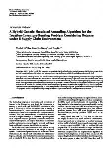
one if facility i is reopened at the beginning of period t, and zero otherwise. The F-chromosome is less important than the L-chromosome (we can say that F-chromosomes complement the information provided by L-chromosomes). Its genes’ values will only be taken into account when strictly needed. We will refer to the (t-1)m+i-th gene in a chromosome as F or L-chromosome[t,i] gene. Consider the following example, with m equal to 5 and T equal to 3 (the matrix notation is used for ease of understanding): Chromosome L i
Chromosome F
1
2
3
4
5
1
1
0
0
1
1
2
1
1
0
0
3
1
1
0
1
t
i
1
2
3
4
5
1
1
1
0
0
1
0
2
0
0
0
1
1
0
3
1
0
1
0
1
t
Figure 1: An individual’s representation
In terms of location variables, these two chromosomes would be interpreted as all variables 2 3 3 3 , r13 , a 22 , a141 , r43 , a151 . The three F-chromosome genes represented equal to zero except a11
in bold italic are the only genes (from this chromosome) that really matter for building the solution. Definition 1: Consider two individuals that differ only in one L (F) - chromosome gene. If the solutions they represent in the phenotype space are different then the L (F) - chromosome gene is called determinant, otherwise is called non-determinant. Proposition 1: All L-chromosome genes are determinant. Proposition 2: The only F-chromosome genes that are determinant are genes in position (t-1)m+i, for some i and
t>1, such that L-chromosome genes (t-1)m+i and (t-2)m+i are equal to one. Proposition 3: It is possible to represent each and every admissible solution to CDLPOCR using a pair of F and
L-chromosomes.
It is straightforward to conclude that this representation is redundant, according to the definition of Rothlauf and Goldberg, 2002: representations are redundant if the number of genotypes exceeds the number of phenotypes. Looking at the previous example, there are a number of different individuals (in the genotype space) that will be mapped to the same solution (in the phenotype space): all individuals that differ from the individual depicted in figure 1 in, at least, one non-determinant F-chromosome gene. Nevertheless, two individuals 13
are mapped to the same solution if and only if their L-chromosomes are exactly the same (due to proposition 1). Rothlauf and Goldberg, 2002 study the effect of redundant representations in the performance of genetic and evolutionary algorithms. Some authors have the opinion that each solution should be coded by exactly the same number of different individuals. The justification is obvious: if some solutions are “super-represented” by several different individuals then the genetic search can be biased. Rothlauf and Goldberg say that synonymously redundant representations, i.e, representations where the genotypes that represent the same phenotype are very similar to each other, do not change the performance of genetic algorithms as long as all phenotypes are represented on average by the same number of different genotypes. We have not studied deeply this problem, but the computational experiments already made let us believe that this is happening in our algorithm (maybe because the L-chromosome genes are all determinant). As can be easily observed, this representation guarantees that restrictions (5), (7) and (8) are satisfied for every individual in the population. The only restrictions that can be violated are the capacity restrictions (11), (12), and (13). Let us now return to problem CDLPOCR and consider the existence of facilities of type 4. Instead of creating another representation for non-binary location variables, we chose to adopt the representation just described to this new situation: a facility i can be composed of up to Nmax elements of equal or different dimensions. This means that, at each time period, there are
at most Nmax elements of each possible dimension. Therefore, to extend the representation to this kind of facilities, each facility i will be represented by q×Nmax genes at each time period t. Each facility i∈I4 is transformed in q×Nmax facilities called dummy facilities. As an example, consider that all facilities are of type 4, T is equal to one, m is equal to 3, q is equal to 4 and Nmax is equal to 2. Then each chromosome would have m×q×Nmax genes, i.e, would have 24 genes and organized as follows: 1
2
s=1
3
4
s=2
5
6
s=3
Facility 1
7
8
s=4
9
10
s=1
11
12
s=2
13
14
s=3
Facility 2
15
16
s=4
17
18
s=1
19
20
s=2
21
22
s=3
23
24
s=4
Facility 3
Figure 2: schematic representation of a chromosome when there are facilities of type 4
14
This representation can be easily translated to decision variables’ values: variables risξτ are equal to the number of dummy facilities corresponding to facility i and dimension s operating from τ to ξ. From all variables risξτ with values greater than zero, we choose risξτ ' such that
{
}
ξ τ ' = min risξτ : risξτ > 0 , and decrease this variable in one unit, changing ais τ ' from zero to one. τ ,s
Notice that for each dummy facility i’ corresponding to facility i∈I4 and dimension s∈S, we can ξ ξ ξ define FRiξ' τ equal to FRis τ and FAi' τ equal to FAisτ . The problem CDLPOCR could be
formulated using only variables aiξτ and riξτ , with i=1,…, #I1+#I2+#I3+q×Nmax#I4. This representation does not guarantee the satisfaction of restrictions (10) nor (14). It has the advantage of maintaining the use of a binary alphabet, and allows the use of simple genetic operators. It has the disadvantage of increasing the number of genes in each chromosome. 3.2
Evaluation Function
In our algorithm, the fitness of each and every individual in a population is equal to the objective function value of the corresponding solution in the phenotype space. The calculation of the fixed open and reopen costs comes out directly from the solution’s representation. Algorithm 1 describes this procedure for facility i. If i∈I4 then this algorithm will be used for each of the q×Nmax dummy facilities and the costs summed up. After deciding which variable ξ ais τ ' is equal to one (as described in the preceding section), then the total cost is changed by ξ ξ summing FAis τ ' minus FRisτ ' .
The assignment costs are calculated separately as described in section 2. If the allocation problem (that has to be solved if in presence of capacitated facilities) is impossible, then the solution will have fitness equal to +∞. The same happens if restrictions (10) are violated. Algorithm 1: Calculation of fixed open and reopen costs for facility i
1. cost ← 0; open ← false; t ←1. 2. If t > T then stop, else go to 3. 3. if L-chromosome[t,i]=false then t ← t+1 and go to 2; else go to 4. 4. tin ← t; t ←t + 1; 5. If L-chromosome[t,i]=1 then go to 6; else go to 7. 6. If F-chromosome[t,i]=1 and tin ≠ t then go to 7, else t ← t+1 and go to 5. 7. tend ←t − 1. 15
tend 8. If not open and i∉I4 then open ← true, cost ← cost + FAitend tin ; else cost ← cost + FRi tin .
Go to 2. 3.3
Genetic Operators
The genetic algorithm developed uses the most common genetic operators found in the literature: selection, crossover and mutation. We also developed some special operators that take advantage of the known structure of the problem, namely a repair algorithm (that diminishes the number of non-admissible individuals) and an algorithm that changes only the F-chromosome’s genes (and tries to diminish the solution’s fixed open and reopen costs).
In the next sub-sections all these genetic operators will be described. 3.3.1
Selection
The selection operator used is based on binary tournament selection with sharing (Goldberg, 1989, Oei et al, 1991, Deb, 2001). In every generation, two individuals are randomly selected from the parent population. A sharing value is calculated for each of them. This sharing value is used to prevent the early convergence of the population towards a single solution, and is calculated as follows: given two individuals i and j, the distance between them is given by the number of L-chromosome genes that are different in both individuals. 1, if the ϑ − gene in the L - chromosome is different in i and j d ijϑ = 0, otherwise d ij =
mT
∑ d ijϑ
ϑ =1
d ij sh(i , j ) = 1 − α share 0 ,
α
, if d ij ≤ α share otherwise
For each selected individual i, all values sh(i,j) 13 (calculated considering all individuals j belonging to the new – children – population ) are summed up: nci =
∑ sh(i , j )
j belongs to the new population
If, at the moment of the selection, there are already num individuals in the new population, then nci = num–nci. The individual’s fitness value will be divided by nci, and the resulting value
13
The αshare value is calculated as described in Deb, 2001 and α is considered equal to one.
16
(f(i)) is used in the binary tournament selection. In the presence of two randomly chosen individuals x1 and x2, if f ( x1 ) < f ( x 2 ) then individual x1 wins the binary tournament with a given probability pbt14. 3.3.2
Crossover
The crossover operator used is an adaptation of the one-point crossover. Two parent solutions will be recombined yielding two children. A value κ between 1 and T is randomly chosen. The first child will have all L and F-chromosome genes (t-1)m+i, with t< κ, equal to the first parent, and all the other genes equal to the second parent. The opposite happens with the second child. This operator guarantees that if two parents satisfy restrictions (10), then so will their children. However, this crossover operator does not guarantee that the children of two admissible parents are admissible. 3.3.3
Mutation
The mutation operator is responsible for random changes in an individual’s genotype. According to Goldberg, 1989, mutation is simply an insurance policy against the loss of genetic material. Each L and F-chromosome gene is changed with a given mutation probability pµ (usually close to zero). For each facility of type 4 only one L and one F-chromosome gene (randomly chosen) can be changed by the mutation operator in each time period. 3.3.4
Additional genetic operators
The algorithm developed tries to take advantage of all the existing knowledge about the problem at hand. This is why two more operators were designed: one operator is a repair algorithm that tries to diminish the number of inadmissible solutions in every generation. The computational experiments showed that, without a repair algorithm, the populations had a large number of inadmissible solutions (especially in presence of facilities of type 3 or 4) that were responsible for a weak performance (this is in accordance with Davis, 1996: a genetic algorithm that generates many illegal - not admissible - solutions will always perform worse than an algorithm that generates no illegal solutions). The other operator tries to change F-chromosome determinant genes in order to diminish the fixed open and reopen costs.
14
This probability is usually close to 1.
17
3.3.4.1
The Repair Procedure
An individual represents an inadmissible solution if: 1. it violates any maximum or minimum capacity restrictions; 2. the total number of elements located at a facility i of type 4 is greater than Nmax. These violations are caused by L–chromosome genes. The repair algorithm changes in a random but guided manner L-chromosome genes, as depicted in algorithm 2. If maximum capacity restrictions are violated at period t it randomly opens more facilities (changes genes from zero to one) such that the minimum capacity restrictions remain satisfied. If minimum capacity restrictions are violated at period t it randomly closes facilities (changes genes from one to zero) such that the maximum capacity restrictions remain satisfied. If there are facilities of type 3, then the allocation problem cannot be split into T separate problems. In this case, a heuristic procedure is used to achieve admissibility. If the maximum number of equipments placed at i (being i a facility of type 4) is exceeded, then the repair algorithm randomly chooses genes i’ equal to one that correspond to elements of i and change their values to zero.
As all changes are performed in a random manner, the repair algorithm cannot guarantee to find an admissible solution. That is why a maximum number of tries had to be imposed. We chose to repair an infeasible solution in a random manner because the use of a more structured algorithm (like a greedy heuristic) can introduce a strong bias in the search (Coello Coello, 2002). 3.3.4.2
The Change Opening procedure
This procedure studies the effect on fixed (re)open costs of changes in some of the determinant F-chromosome genes. As stated in proposition 2, we can identify an F-chromosome determinant gene if the L-chromosome genes in the same and in the
immediately previous time position are equal to one for some facility i. The procedure does not try to change every determinant F-chromosome gene, because that would be very time consuming. It only identifies situations such that a facility i is open from the beginning of time period τ to the end of time period ξ, ξ > τ, and is reopen during that interval (in a time period t ≤ ξ). This means that there is a determinant F-chromosome gene in position (t-1)m+i that is equal to one, and this is the gene whose value the procedure tries to change to zero. If the fixed open and reopen costs diminish, then the gene’s value is changed, otherwise retains its original value.
18
Algorithm 2: Repair Algorithm Predefined parameters: NMAXTRY-total number of iterations in each time period.
1. If there are facilities of type 3 then go to 2. Else go to 3. 2. Solve the total assignment problem using a general solver. If the problem is impossible then go to 3, else stop (the solution is admissible). 3. t ←1. For each facility i∈I3, calculate Capi0 ←0. 4. ntries ←1. If t > T then stop. Else go to 5. 5. For each facility i∈I3 update:
[ ]
Capit −1 + Qi , if L - chromosome t,i = 1 and F t Capi ← Capit −1 , otherwise
- chromosome[t,i ] = 1
.
This value represents the maximum capacity of facility i during period t. 6. Calculate D ← ∑ d tj , Cmax← total maximum capacity of facilities operating during t15, j
Cmin← total minimum capacity of facilities operating during t, Numi ← total number of
elements operating at i∈I4, during t, ∀i∈I4. 7. ntries ← ntries + 1. If ntries > NMAXTRY then stop. Else go to 8. 8. If Cmin>D then go to 9. If Cmax < D then go to 10. If ∃i∈I4: Numi > Nmax then go to 11. Else go to 13. 9. Choose randomly a facility i∈I2 such that L-chromosome[t,i]=1 and Cmax−Qi ≥ D. L-chromosome[t,i] ←0, Cmin←Cmin − Q' i , Cmax←Cmax−Qi. Go to 7.
10. Choose randomly a facility i (including dummy facilities) such that L-chromosome[t,i]=0 and
Cmin+ Q' i
≤
D16.
L-chromosome[t,i]
←1,
Cmin←Cmin + Q' i .
If
i∈I3
then
Cmax←Cmax+ Capit , else Cmax←Cmax+Qi17. If i is a dummy facility then Numi’ ← Numi’+1,
with i’ the corresponding facility belonging to I4. Go to 7. 11. Choose randomly a facility i∈I4 such that Numi > Nmax. 12. Choose randomly a dummy facility i’ corresponding to one open element in i of dimension s, s ∈ S. L-chromosome[t,i’] ←0, Numi ← Numi −1, Cmax←Cmax−Qs.
15
If there is at least one facility of type 1 in operation during t, then Cmax←+∝.
16
If i∈I3 or is a dummy facility, then Q' i is equal to zero.
17
If i is a dummy facility corresponding to dimension s, then Qi will be equal to Qs.
19
13. If there are no facilities of type 3, then t ← t+1 and go to 4. Else go to14. 14. Solve one transportation problem as described in section 2, treating facilities of type 3 as facilities of type 2 with maximum capacities equal to Capit and minimum capacities equal to zero. Update Capit ,∀i ∈ I 3 , subtracting the total flow that reaches demand point i. t ← t+1 and go to 4.
This procedure does not change F-chromosome genes corresponding to facilities of type 3, because it could not only change the fixed costs value but also the allocation problem’s optimal solution. In algorithm 3, the change opening procedure is formally described.
Algorithm 3: Change-Opening procedure
1. i ←1; 2. If i∈I3 then i ←i + 1. 3. If i > m, then stop. If i∉I4 go to 4, else go to 6.
(
) (
)
4. Detect a pair of location variables equal to one of the form aiξτ , riψξ +1 or riξτ , riψξ +1 . If there are no pair of variables in this situation, then i ← i + 1 and go to 3. Else go to 5.
(
)
)
(
ψ ξ ξ ψ 5. ∆ ← FAψ iτ or FRiτ − FAiτ or FRiτ − FRiξ +1 . If ∆