A Hybrid Feature Selection and Generation Algorithm for ... - CiteSeerX

2013 12th International Conference on Machine Learning and Applications

A Hybrid Feature Selection and Generation Algorithm for Electricity Load Prediction using Grammatical Evolution Anthony Mihirana de Silva, Farzad Noorian, Richard I. A. Davis, Philip H. W. Leong School of Electrical and Information Engineering, University of Sydney, Sydney, NSW 2006, Australia {anthonymihirana.desilva, farzad.noorian, richard.davis, philip.leong}@sydney.edu.au

A framework for function-based feature generation using context-free grammars was first proposed by Markovitch and Rosenstein [2]. Such grammars are used in linguistics to describe sentence structure and words of a natural language and in computer science to describe the structure of programming languages. Markovitch and Rosenstein generated features strongly related to the target using decision trees. Unfortunately, the technique was only suitable for problems where the features are apparent from the problem definition. In other related work, Eads et. al [3] and Pachet and Roy [4] addressed supervised time-series classification using genetic programming (GP) operators defined in a grammatical structure. GP was also used by Ritthof et. al [5] to combine feature generation and selection and applied to the interpretation of chromatography time-series. Automatic feature generation can generate irrelevant and redundant features. Feature selection (FS) eliminates such features thereby improving the accuracy and speed of ML algorithms. Genetic algorithms have been used for FS as a so called wrapper to avoid enumerating the entire space [12]– [14]. Muni et. al. [15] proposed a GP based FS algorithm which evolved a population of classifiers to choose accurate classifiers with the minimum number of features. Multipopulation GP has also been used in [16] to develop a method for simultaneous feature extraction and selection. In this paper, we use a modified version of grammatical evolution (GE) [17] to generate and select parametrized features for peak electricity load prediction. Some of the generated features in this work use the concept of technical indicators, as used in finance. These are formulae that identify patterns and market trends in financial markets, developed from models for price and volume. To the best of our knowledge, this is the first time (i) GE is applied as a feature discovery technique in time-series prediction, and (ii) technical indicator type formulae are used for predicting

Abstract—Accurate load prediction plays a major role in devising effective power system control strategies. Successful prediction systems often use machine learning (ML) methods. The success of ML methods, among other things, depends on a suitable choice of input features which are usually selected by domain-experts. In this paper, we propose a novel systematic way of generating and selecting better features for daily peak electricity load prediction using kernel methods. Grammatical evolution is used to evolve an initial population of well performing individuals, which are subsequently mapped to feature subsets derived from wavelets and technical indicator type formulae used in finance. It is shown that the generated features can improve results, while requiring no domain-specific knowledge. The proposed method is focused on feature generation and can be applied to a wide range of ML architectures and applications. Keywords-Load prediction; grammatical evolution; feature selection; context-free grammar; machine learning

I. I NTRODUCTION Electricity load prediction is the first phase in power system planning and control. While overestimation leads to an undesired spinning reserve and excess supply, underestimation causes insufficient reserve supply, implying higher costs. The inherent non-linear and non-stationary nature of electricity load time-series makes supervised machine learning (ML) methods more appealing for prediction than model-based approaches [1]. In a time-series prediction task, the ML algorithm is presented with training samples (x1 , y1 ), (x2 , y2 ), . . . , (xn , yn ), where x j ∈ RN is a vector of input features and y j ∈ R is the target, e.g. daily peak electricity load. The learner has to infer a general function (a hypothesis) that can predict yk for unseen xk . This generalization is achieved by searching a hypothesis space H for a solution hypothesis h ∈ H that best fits the structure of the training samples. The performance of ML algorithm depends strongly on the formalism of h using different input feature vectors, x. The input features used in some electricity load prediction applications are summarised in Table I. In each case, the input features selected by human experts were similar with some overlap between different works. However, the choice is generally ad-hoc. It would therefore be useful to have a framework that can automatically generate and select useful features that have a meaningful interpretation. 978-0-7695-5144-9/13 $31.00 $26.00 © 2013 IEEE DOI 10.1109/ICMLA.2013.125

Table I: Common features in electricity load time-series prediction. • • • • •

211

Previous week’s hourly load information Temperature and calendar information Previous load information and its differenced values Daubechies wavelets and its differenced values EMD transform and its differenced values

[6]–[8] [9], [10] [11]

Starting Element

Final Terminal Element

< expr >

((lag(H, k)) − (lag(C, k)) ÷ ((lag(H, k)) − (lag(L, k)))

(1.a)

(5.b)

(< der − var >) < op > (< der − var >)

((lag(H, k)) − (lag(C, k)) ÷ ((lag(H, k)) − (lag(< var >, k)))

(2.a)

(3.a)

((< var − op >) < op > (< var − op >)) < op > (< der − var >)

((lag(H, k)) − (lag(C, k)) ÷ ((lag(H, k)) − (< var − op >))

(3.a)

(4.b)

((lag(< var >, k)) < op > (< var − op >)) < op > (< der − var >) (5.a)

((lag(H, k)) − (lag(C, k)) ÷ ((lag(H, k)) < op > (< var − op >))

((lag(H, k)) < op > (< var − op >)) < op > (< der − var >) (4.b)

(5.a) ((lag(H, k)) − (lag(C, k)) ÷ ((lag(< var >, k)) < op > (< var − op >))

((lag(H, k)) − (< var − op >)) < op > (< der − var >) (3.a) ((lag(H, k)) − (lag(< var >, k)) < op > (< der − var >) (5.c) ((lag(H, k)) − (lag(C, k)) < op > (< der − var >)

(3.a) ((lag(H, k)) − (lag(C, k)) ÷ ((< var − op >) < op > (< var − op >)) (2.a) (4.a)

((lag(H, k)) − (lag(C, k)) ÷ (< der − var >)

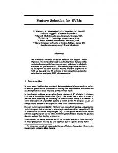
Figure 1: Feature generation using GE. The circles represent the leftmost non-terminal to apply the production rules on. The rules are chosen based on the MOD operator result on codons. If the first codon of the chromosome is 224, since the first non-terminal is and the number of rules available in grammar family 2 is 2, the rule is (224) MOD (2) = 0, hence rule (1.a) is chosen, and so on.

as production rules) in the form of R → α with R ∈ N , α ∈ (N ∪ T ). S ∈ N is the start symbol. If rules are defined as R = {x → xa, x → ax}, a is a terminal symbol since no rule exists to change it, and x is a non-terminal symbol.

electricity load time-series. Define the solution hypothesis of a particular ML architecture formulated using expert suggested features h1 and the solution hypothesis formulated using a feature subset discovered through the proposed framework h2 . The main contribution of our work is to demonstrate that the prediction accuracy can be better with h2 than with h1 . This paper is organized as follows. Sec. II provides a brief review of context-free grammar and GE. Sec. III presents the main part of our work on how grammar families are evolved to generate informative features. The results are given in Sec. IV and the performance of our approach is compared with other approaches. Finally, the paper is concluded with remarks for future work in Sec. V.

B. Grammatical Evolution GE is a grammar-guided GP technique, which has been used in computational finance, credit rating & corporate failure prediction, music and robot control applications (refer to [19] for a survey). GE can be used to evolve complete programs in an arbitrary language. Similar to GP, GE evolves a population towards a certain goal. GE performs evolutionary operations on integer individuals which are then mapped using the defined grammar to feature subsets; on the other hand GP directly operates on the actual program’s tree structure [17]. In GE, a suitable grammar developed for the problem at hand is specified in BNF. A chromosome is represented as an integer string, with each integer creating a codon. The codon values are then used to select production rules from the grammar definition using the modulus (MOD) operator. A group of codons which is used to create a feature is called a gene. Detailed explanation on GE can be found in [17] and is omitted here for space. Fig. 1 illustrates how the grammar family 2 in Table II can generate a feature. With C lagged by k = 1 and L and H lagged by k = 0, we obtain (Ht − Ct−1 )/(Ht − Lt ). This formula is popular as the accumulation/distribution oscillator which is a widely used technical indicator by financial analysts. The proposed grammar can produce many such popular indicators.

II. BACKGROUND A. Context-free Grammar A context-free grammar (CFG) is used to generate patterns and strings using hierarchically organized production rules [18]. Using the Backus-Naur form (BNF), a CFG can be described by the tuple (T , N , R , S ) where T is a set of terminal symbols and N is a set of non-terminal symbols with N ∩ T = ∅. The non-terminal symbols in N and terminal symbols in T are the lexical elements used in specifying the production rules of a CFG. A non-terminal symbol is one that can be replaced by other non-terminal and/or terminal symbols. Terminal symbols are literals that symbols in N can take. A terminal symbol cannot be altered by the grammar rules R , a set of relations (also referred to

212

III. METHODOLOGY

enabling the usage of wavelet coefficients as features. The m-level wavelet decomposition coefficients of x(k) are D j (k) and S j (k), j = 1, 2, . . . , m. The D coefficients capture local fluctuations and S are smoothed (trend) versions at each scale. The mth level wavelet decomposition of a time-series n n is then given by: Dm = ∑ Dm (k+i) and Sm = ∑ Sm (k+i). The i=0 i=0 grammar in Table III uses wavelets. H is the maximum daily electricity load time-series. D1 , D2 , D3 and S = S3 are the 3-level decomposition components of H. Empirical mode decomposition (EMD) is an alternative to wavelets but an EMD based grammar was not used for this paper.

Fig. 2 shows the proposed architecture. Chromosomes are selected from the population which are then mapped to feature subsets using CFG in Tables II and III. These subsets are evaluated and best feature subsets are selected by a wrapper approach. The population is evolved such that the learner architecture has a minimum mean cross validation error on randomized samples drawn from a validation set. Evolutionary Operators

Initial Population

Exit

Mutation

Table II: High, low, close electricity load multi-family grammar.

Yes

Cross-over

Grammar family 1 (moving average)

Chromosome

Selection

No

N = {expr, der-var, base-var, pre-op, base-op, var} T = {÷, delt, diff, ema, sma, max, min, meandev, H, L, C, n, (, ) } S =

Criteria?

CFG Feature Subsets

ML Algorithm

Fitness

R Production rules

Feature Subset Goodness Evaluation

expr

Figure 2: The architecture of the prediction system.

A. Grammar Definition The grammar families in Table II can generate trend, momentum and volatility type indicators. This grammar construction was inspired by 30 common technical indicators. A single grammar capable of generating all the features generated by the grammar families can be designed but such a grammar would have many production rules, leading to a large search space and long computational times. In the financial literature, data is represented by H, L and C which are the daily highest, lowest and closing (last) prices. The upward and downward price changes are U = max(0, Ht − Ht-1 ) and D = min(0, Ht − Ht-1 ), Ht is the current time-sample highest price. In this paper, the same notation is adapted to half-hourly electricity load data, with the daily high, low and close electricity load used in place of price. The basic operators lag, abs, diff and delt respectively refer to lagged (xt−k ), absolute (|xt |), first difference (Δx = xt − xt−1 ) and the relative first difference values ((xt − xt−1 )/xt ) of a time-series where xt is the load at time t and k is a constant. The operators ema, sma, max, min, sd, meandev and histwin extract the exponential moving average, simple moving average, maximum, minimum, standard deviation, mean deviation and a history sequence for a moving window of size n. The discrete wavelet transform is widely used as a multi-resolution decomposition technique which can elucidate otherwise hidden relationships in non-stationary timeseries like electricity load data. We perform the maximal overlap discrete wavelet transform using the Daubechies mother wavelet. For a time-series x(k) with N samples, each resolution scale would have N samples for each level,

der-var base-var

::= (expr)÷(expr) | der-var | base-var (1.a), (1.b), (1.c) ::= pre-op(base-var, n) (2.a) ::= base-op(var) | pre-op(var, n)| var (3.a), (3.b),

pre-op base-op var

(3.c) ::= ema | sma | max | min | meandv ::= delt | diff ::= H | L | C

(4.a), (4.b), (4.c), (4.d), (4.e) (5.a), (5.b) (6.a), (6.b), (6.c)

Grammar family 2 (momentum)

N = {expr, der-var, var-op, op, var} T = {÷, -, lag, ema, U, D, H, L, C, n, k, (, ) } S = R Production rules expr der-var var-op op var

::= ::= ::= ::= ::=

der-var÷der-var (1.a) var-opopvar-op | var-op (2.a), (2.b) lag(var, k) | ema(var, n) (3.a), (3.b) ÷|(4.a), (4.b) H|L|C|U|D (5.a), (5.b), (5.c), (5.d) (5.e), (5.f) Grammar family 3 (volatility)

N = {expr, var-op, var} T = {+, -, abs, sma, sd, H, L, C, n, (, ) } S = R Production rules expr var-op var

::= sma(var-op, n) + sd(var-op) (1.a) | sma(var-op, n) - sd(var-op) (1.b) ::= abs(var) | var (2.a), (2.b) ::= H-L | H-C | C-L | H (3.a), (3.b), (3.c), (3.d)

B. Feature Generation Feature generation is guided through GE. Each chromosome is dissected to 25 genes where each gene is considered a feature and GE is applied independently on each gene. To have a good mix of trend, momentum and volatility type formulae in HLC grammar, the first 10 gene partitions were

213

information to the feature subset. Temperature information was not used since we investigated the effect of features derived from the time-series history itself.

Table III: Wavelet based grammar. N = {expr, der-var, base-var, pre-op, base-op,var} T = {abs, delt, diff, lag, sma, sd, meandev, histwin, H, D1 , D2 , D3 , S, n, k, (, )}

S =

C. Feature Subset Evaluation

R Production rules

The last step of the procedure was to evaluate the performance of a generated feature subset. Some of the generated features were parametrized by the window-size n = 2, 3, 5, 7, 14 and lag k = 0, 1, 2, 3, 4, 5, 6, 7, 14.

expr der-var base-var pre-op base-op var

::= histwin(base-var, n) | der-var | base-var ::= pre-op(base-var, n) ::= base-op(var) | lag(var, k) | pre-op(var, n) ::= sma | sd | meandev ::= delt | diff | abs ::= H | D1 | D2 | D3 | S

(1.a) (1.b) (1.c) (2.a) (3.a) (3.b) (3.c) (4.a), (4.b), (4.c) (5.a), (5.b), (5.c) (6.a), (6.b), (6.c), (6.d), (6.e)

Algorithm 1 Feature subset evaluation procedure Input current integer chromosome 1: Extract individual genes from the current chromosome 2: Map genes into grammar families (if necessary) 3: Derive symbolic features 4: Generate numeric feature subset Yk for each time stamp 5: Append calendar information to Yk (see Sec. IV) 6: for i in 1:N do 7: err[i] = ML algorithm MAPE in validation sample i 8: end for 9: Calculate the average MAPE e(Yk ) = mean(err) 10: Calculate the final score J(Yk ) = e(Yk ) + q(Yk ) + c(NNT ) Output J(Yk )

mapped to the moving average grammar family, the next 10 to the momentum family and the final 5 to the volatility family. A single grammar was used for wavelet based feature generation with no such gene mapping. Individuals were selected for recombination using fitness proportionate selection (also known as roulette wheel selection). We employed random mutation and a modified version of multiple-point crossover, such that the crossover is performed across all individual genes (see Fig. 3). The chromosome is represented as set of stacked genes for clarity. This crossover ensures that inter-grammar-family crossover is avoided. Elite individuals, i.e. the chromosomes that rank best in each generation were passed directly to the next generation without mutation or crossover. Parent 1

The feature subset evaluation steps are shown in Algorithm 1. The individuals with the lowest score were (mean absolute deemed to be the best. e(Yk ) is the MAPE n  y −yˆ  i i  where n is the number percentage error), given by 100  ∑ n yi i=1 of predictions, y is the target and yˆ is the predicted value. To choose robust features providing good generalization, the mean MAPE was calculated by the average error on N = 15 random samples of size 30 drawn from a validation dataset, e.g. the validation dataset Oct. 1998 - Dec. 1998 for predicting Jan. 1999. q(·) is an assessment of the symbolic feature expression complexity, taking into account the length, the number of operations and pre-operations. c(·) was calculated based on the number of non-terminal elements NNT in subset Yk (a subset containing many nonterminal elements was considered as poor).

Parent 2 Gene 1 Gene 2

n integers in N partitions

....... Gene n

Cross-over points Child 1

Child 2

N partitions

Child 1 unwrapped n integers

IV. RESULTS

Figure 3: The proposed multiple-point crossover approach. A random number of crossover points at random locations are chosen.

The EUNITE dataset [20] has been extensively used as a benchmark to test load prediction algorithms. It was originally published for a competition to predict the peak daily load for January 1999 using half-hourly recordings in the years 1997 and 1998. In our approach, first the data was scaled to ensure that each feature was independently normalized. Calendar information was encoded as 7 binary values to represent the day-of-week and a single binary value for holidays as the competition winners in [6]. A self organising map (SOM) was used to identify data clusters using a peak load history window of 7 days, temperature and calendar information as

We placed some specific chromosomes in the initial population which map to subsets of standard technical indicators such as disparity, momentum, stochastic oscillator (K), stochastic indicator (D), William’s oscillator (R), ROC (rate of convergence), RSI (relative strength index), CCI (commodity channel index) and moving averages. This ensured that the initial population was healthy and encouraged the generation of high performing feature subsets. The rest of the population consisted of randomly generated individuals. In making the final predictions, we also added calendar

214

SOM inputs. This showed a very strong seasonality, dividing the data into cold and hot seasons (season 1 and 2 in Fig. 4 respectively). Based on the SOM result, we only used data from season 1 months to construct models in our experiments, e.g. to predict Jan. 1999, the model was constructed using Jan. 1997 - Mar. 1997, Oct. 1997 - Mar. 1998 and Oct. 1998 - Dec. 1998 data. Season 2

600

700

800

Season 2

performed remarkably well only in Jan. 1999 but the average accuracy was inferior to other subsets considered. We suspect that some related work on the EUNITE dataset have used specific subsets in a trial and error fashion to report good performance only on the test dataset, Jan. 1999. A chromosome of the proposed GE algorithm comprised of 24 codons and 25 genes, i.e. a total 25 features with each feature represented by 24 codons making the integer chromosome size 600. The population size was 24 and 100 generations were iterated. The best 2 chromosomes in each generation were considered to be elite individuals. 10 GE trials were performed and the results are brought at the bottom of Table IV. The HLC based grammar produced significantly better results for each of the 3 months (1.15%, 1.73% and 1.39%), and even the worst performing HLC feature subset outperformed all other methods for average day-ahead predictions. Although the best wavelet feature subset (1.81%) outperformed other domain-expert suggested feature subsets for day-ahead predictions, the average performance of each month (1.96%) was poor. However, its performance for month-ahead prediction was promising. This leads us to state that the HLC grammar incorporates more information about the daily variations of load and significantly improves day-ahead predictions while the wavelet grammar elucidates long-term trends and hence is more suited for month-ahead predictions. Table V compiles selected features from all GE trials filtered using the minimum-redundancy-maximum-relevance (mRMR) criterion. While some features are obvious and straightforward (e.g. ΔH, H, delt(H), histwin(H, 14)),

Season 1

Season 1

500

Season 1

Jan 01 1997

Apr 01 1997

Jul 01 1997

Oct 01 1997

Jan 01 1998

Apr 01 1998

Jul 01 1998

Oct 01 1998

Jan 01 1999

Figure 4: Clustering days to different seasons using a SOM.

Two different experiments were performed on the dataset. In the first trial, we used the wavelet based grammar in Table III in a month-ahead manner of prediction. Here, after predicting a load value for January 1st , 1999, we used this predicted value with the historical values before January 1st to predict January 2nd , 1999. This process was continued until the predicted load value of January 31st was obtained. For the second approach, we used the grammar in Table II. This requires the previous day’s high, low and close values, and is more suited to a day-ahead prediction approach. Therefore, the actual historical HLC values are used in predicting each day. For initial performance comparison, autoregressive integrated moving average (ARIMA) and exponential smoothing (ETS) models were chosen as analytical methods. Support vector machine (SVM) and kernel recursive least squares (KRLS) algorithm were used as kernel based ML methods. Table IV summarizes the results of the different techniques used for different feature subsets on different months. It was observed that the best results were produced by kernel methods with a radial basis kernel function parametrized by γ, i.e. K(xi , x j ) = exp(−γxi − x j 2 ), where xi , x j are the input training vectors, i, j = 1, 2, . . . , m. As KRLS requires one less parameter (σ and λ) than SVM regression (C, γ and ε) consuming less hyper-parameter tuning time, KRLS was chosen for feature subset evaluation as explained in section III-C. The optimal parameters for the KRLS feature subset evaluator, σ = 256 and λ = 0.0625 were chosen by 10-fold repeated cross validation using a peak load history window of 7 days and encoded calendar information as features. Based on the features used in previous load prediction work, we compared the performance of 5 domain-expert suggested feature subsets in Table IV and observed that the result stability for different months is poor, e.g. the feature subset Hk , ΔHk , ΔD1i , ΔD2i , ΔD3i , ΔSi (∀i ∈ {k − 1, ..., k − 6})

Table V: Selected features from 10 GE runs.

1 2 3 4 5 6 7 8 9 10 11 12 13 14 15 16 17 18 19 20 21 22 23 24 25

215

HLC features

Wavelet features

(|C-L|-|L|)/|C-L| (|L|-|H-L|)/L (ema(ΔC, 2))/(ema(delt(C), 2)) (ema(H, 5))/(min(ema(H, 2), 2)) delt(H) delt(L) ΔH ema(C, 3) ema(C-L, 5) + sd(H-L, 3) ema(D, 3) ema(ema(H, 5), 3) ema(H, 7) ema(H, 7) - sd(H-C, 2) ema(H-C, 2) + sd(H, 14) ema(lag(D,7), 3) ema(lag(U, 3), 3) lag(H, 7) lag(U, 1) max(H, 14) max(L, 3)-lag(H, 7) max(lag(H, 1), 3) min(D, 5) min(ΔC, 5) sd(H, 5)-lag(D, 7) sma(ΔL, 2)

D1 delt(H) ΔD1 ΔH ΔS H lag(D3 , 5) lag(delt(H), 2) lag(ΔD1 , 1) lag(ΔD3 , 4) lag(meandev(D1 , 14), 3) lag(sd(H, 7), 3) lag(S, 6) lag(sma(D1 , 7), 6) histwin(ΔH, 7) lag(sma(H, 5), 4) histwin(H, 14) meandev(D1 , 14) sd(D1 , 14) sd(H, 14) S sma(D1 , 14) sma(D1 , 7) sma(D2 , 3) sma(D3 , 3)

Table IV: Kernel method performance comparison for different feature subsets on 3 different months. Method and Features

Month-ahead MAPE %

Day-ahead MAPE %

Jan. 1999 Dec. 1998 Nov. 1998 Avg. Jan. 1999 Dec. 1998 Nov. 1998 Avg. Last Year’s Data ARIMA ETS

2.29 2.08 1.87

4.79 4.97 4.66

3.22 3.45 3.47

3.43 3.50 3.33

2.29 2.60 2.11

4.79 2.55 2.48

3.22 2.71 2.10

3.43 2.62 2.23

Linear SVM with Hi (∀i ∈ {k, ..., k − 6}) Polynomial SVM with Hi (∀i ∈ {k, ..., k − 6}) Radial SVM with Hi (∀i ∈ {k, ..., k − 6}) Polynomial KRLS with Hi (∀i ∈ {k, ..., k − 6}) Radial KRLS with Hi (∀i ∈ {k, ..., k − 6})

2.32 2.22 1.96 3.93 1.67

3.84 3.50 2.87 4.71 3.06

1.82 1.82 1.75 3.46 1.76

2.66 2.52 2.19 4.03 2.16

1.62 1.72 1.68 3.91 1.61

2.39 2.39 2.19 4.62 2.31

1.99 1.99 1.81 3.38 1.85

2.00 2.03 1.89 3.97 1.92

Using radial KRLS with feature subsets Hi (∀i ∈ {k, ..., k − 6}) + Temp. Hi (∀i ∈ {k, ..., k − 6}) D1k , D2k , D3k , Sk Hk , ΔHk , ΔD1k , ΔD2k , ΔD3k , ΔSk Hk , ΔHk , ΔD1i , ΔD2i , ΔD3i , ΔSi (∀i ∈ {k − 1, ..., k − 6})

3.59 1.67 1.88 1.64 1.55

3.05 3.06 3.25 3.49 3.98

2.06 1.76 1.70 1.96 2.56

2.90 2.16 2.27 2.36 2.70

2.25 1.61 1.62 1.62 1.25

2.52 2.31 2.05 2.08 2.61

1.86 1.85 1.84 1.93 2.25

2.21 1.92 1.84 1.88 2.04

-

-

-

-

1.15 1.34 1.62

1.73 1.89 2.03

1.39 1.56 1.68

1.48 1.60 1.68

1.42 1.82 2.42

2.45 2.89 3.32

1.35 1.54 1.76

1.84 2.08 2.31

1.61 1.77 1.90

1.93 2.31 2.89

1.66 1.79 1.98

1.81 1.96 2.26

HLC grammar - best of each month HLC grammar - average of each month HLC grammar - worst of each month Wavelet grammar - best of each month Wavelet grammar - average of each month Wavelet grammar - worst of each month

in minimising the gap between the best and worst performing feature subsets in Table V.

many others are not so apparent to human experts. We defer the interpretation of the features in this paper and make our code and results of individual GE trials available at http://www.ee.usyd.edu.au/cel/ICMLA2013 to facilitate further research as suggested in our conclusion or by any other means.

ACKNOWLEDGMENT This work was supported by the Australian research council under the linkage project LP110200413.

V. CONCLUSION R EFERENCES

In this paper, GE was used to combine the generation and selection of seemingly unconventional input features for electricity load prediction, compactly represented using CFGs. It was found empirically that the approach can improve the 3-month average MAPE for a KRLS based predictor from 1.84% to 1.48% for day-ahead predictions and from 2.16% to 1.84% for month-ahead predictions. Although the EUNITE dataset was used for empirical evaluation, the technique is general and is applicable to many other timeseries applications by defining appropriate CFGs based on domain knowledge. Previous electricity load prediction research has mostly focused on improving different ML algorithms and utilized similar features. This paper described a new approach to automatically generate better features which is independent of the ML algorithm. The approach can be easily applied to other ML architectures as well. By comparing the results to previous work on the dataset [21], we see that even without using any sophisticated ML architectures encouraging results can still be obtained by better formalizing the solution hypothesis using better features. Future research will utilize ensemble FS techniques to ensure that the selected feature subsets are robust for non-stationary time-series and will aid

[1] P. Brockwell and R. Davis, Introduction to time series and forecasting. Springer, 2002. [2] S. Markovitch and D. Rosenstein, “Feature generation using general constructor functions,” in Machine Learning, vol. 49. The MIT Press, 2002, pp. 59–98. [3] D. Eads, K. Glocer, S. Perkins, and J. Theiler, “Grammarguided feature extraction for time series classification,” in Proceedings of the 9th Annual Conference on Neural Information Processing Systems, 2005. [4] F. Pachet and P. Roy, “Analytical features: a knowledge-based approach to audio feature generation,” EURASIP Journal on Audio, Speech, and Music Processing, vol. 1, 2009. [5] O. Ritthof, R. Klinkenberg, S. Fischer, and I. Mierswa, “A hybrid approach to feature selection and generation using an evolutionary algorithm,” in U.K. Workshop on Computational Intelligence, 2002, pp. 147–154. [6] B. J. Chen, M. W. Chang et al., “Load forecasting using support vector machines: A study on EUNITE competition 2001,” IEEE Transactions on Power Systems, vol. 19, no. 4, pp. 1821–1830, 2004.

216

[21] M. Moazzami, A. Khodabakhshian, and R. Hooshmand, “A new hybrid day-ahead peak load forecasting method for iranian national grid,” Applied Energy, vol. 101, pp. 489 – 501, 2013.

[7] M. Espinoza, J. Suykens, and B. De Moor, “Load forecasting using fixed-size least squares support vector machines,” Computational Intelligence and Bioinspired Systems, vol. 1, pp. 488–527, 2005. [8] H. Mao, X. J. Zeng, G. Leng, Y. J. Zhai, and J. Keane, “Short-term and mid-term load forecasting using a bilevel optimization model,” IEEE Transactions on Power Systems, vol. 24, no. 2, pp. 1080–1090, 2009. [9] A. Reis and A. da Silva, “Feature extraction via multiresolution analysis for short-term load forecasting,” IEEE Transactions on Power Systems, vol. 20, no. 1, pp. 189 – 198, Feb. 2005. [10] J. Yao and C. L. Tan, “A case study on using neural networks to perform technical forecasting of forex,” Neurocomputing, vol. 34, no. 14, pp. 79 – 98, 2000. [11] L. Ghelardoni, A. Ghio, and D. Anguita, “Energy load forecasting using empirical mode decomposition and support vector regression,” IEEE Transactions on Smart Grid, vol. 4, no. 1, pp. 549–556, 2013. [12] I. S. Oh, J. S. Lee, and B. R. Moon, “Hybrid genetic algorithms for feature selection,” IEEE Transactions on Pattern Analysis and Machine Intelligence, vol. 26, no. 11, pp. 1424 –1437, Nov. 2004. [13] J. Yang and V. Honavar, “Feature subset selection using a genetic algorithm,” IEEE Intelligent Systems and Their Applications, vol. 13, no. 2, pp. 44–49, 1998. [14] C. L. Huang and C. J. Wang, “A GA-based feature selection and parameters optimization for support vector machines,” Expert Systems with Applications, vol. 31, no. 2, pp. 231 – 240, 2006. [15] D. Muni, N. Pal, and J. Das, “Genetic programming for simultaneous feature selection and classifier design,” IEEE Transactions on Systems, Man, and Cybernetics, Part B: Cybernetics, vol. 36, no. 1, pp. 106 –117, Feb. 2006. [16] J. Y. Lin, H. R. Ke, B. C. Chien, and W. P. Yang, “Classifier design with feature selection and feature extraction using layered genetic programming,” Expert Systems with Applications, vol. 34, no. 2, pp. 1384–1393, 2008. [17] M. O’Neill and C. Ryan, “Grammatical evolution,” IEEE Transactions on Evolutionary Computation, vol. 5, no. 4, pp. 349–358, 2001. [18] M. Sipser, “Context-free grammars,” in Introduction to the Theory of Computation. PWS Publishing, 1997, ch. 2, pp. 91–122. [19] R. McKay, N. Hoai, P. Whigham, Y. Shan, and M. ONeill, “Grammar-based genetic programming: a survey,” Genetic Programming and Evolvable Machines, vol. 11, pp. 365–396, 2010. [20] EUNITE. (2001) World-wide competition within the EUNITE network. [Online]. Available: http://neuron-ai. tuke.sk/competition/

217