A Hybrid Image Compression Technique using

A Hybrid Image Compression Technique using Quadtree Decomposition and Parametric Line Fitting for Synthetic Images Murtaza Khan and Yoshio Ohno Graduate School of Science and Technology, Keio University E-mail:[murtaza,ohno]@on.cs.keio.ac.jp Abstract

several techniques based on discrete cosine transform (JPEG) , wavelet transform (JPEG2000), and fractal coding have been developed. The advancement and availability of new software tools to create and generate synthetic images has raise the interest in research community to investigate and devise better techniques for compression of synthetic images. Synthetic images do not compress well using lossy compression techniques [4]. The two most widely used formats for lossless compression are GIF and PNG. In this paper we presented a new technique for synthetic image compression using quadtree decomposition and parametric line fitting. Since our method is based on Quadtree and Parametric Line, therefore we would call our method (QPL). We compared the performance of our technique with well known lossless image compression techniques, GIF and PNG. Organization of the rest of the paper is as follows: Related work is discussed in section 2. Framework is described in section 3. Section 4 is the most important section and it describes the encoding and decoding algorithms. Experiments and results are presented in Sect. 5. Section 6 gives insight view of the proposed method. Final concluding remarks are in Sect. 7.

This paper presents a new hybrid scheme for image data compression using quadtree decomposition and parametric line fitting. In the first phase of encoding, the input image is partitioned into quadrants using quadtree decomposition. To prevent from very small quadrants, a constraint of minimal block size is imposed during quadtree decomposition. Homogeneous quadrants are separated from non-homogeneous quadrants. In the second phase of encoding, the non-homogeneous quadrants are scanned row-wise. Luminance variation of each scanned row is fitted using parametric line at specified level of tolerance. The output data is entropy coded. Experimental results show that the proposed scheme performs better than well-known lossless image compression techniques for several types of synthetic images, e.g., clip-art, cartoon, animation, scientific plot, medical image etc. keywords: image, compression, quadtree, parametric line, fitting. 1

Introduction

The two broad classes of images are natural and synthetic. Natural images occur in nature and are captured by digital devices like camera. The pixel intensities of natural images vary smoothly and there is correlation in the neighboring pixel values. Synthetic images are computer generated, and include animation, clip-art, cartoons, medical images, text images, maps etc. The pixel intensities of synthetic images do not vary smoothly but contain a small discrete set of values. There are large areas (quadrants) of a uniform color and there are sharp changes in color. The objective of image compression is to reduce redundancy of the image data in order to be able to store or transmit data in an efficient form. Due to extensive research on lossy compression of natural images,

2

Related Work

GIF and PNG are the most prevalent lossless image compression techniques. A concise overview of GIF and PNG image compression techniques is described in following sections 2.1 and 2.2 respectively. 2.1

Graphics Interchange Format (GIF)

The Graphics Interchange Format (GIF) is a lossless 8bit-per-pixel bitmap image format that was introduced by CompuServe in 1987 [13, 4]. GIF images are compressed using the Lempel-Ziv-Welch (LZW) coding [12], a dictionary-based technique to exploit redundancy. The initial size of dictionary is 29 , while this 1

fills up, the dictionary size is doubled, until the maximum dictionary size of 4096 is reached. Afterwards the compression algorithm behaves like a static dictionary algorithm. A more detailed description can be found in [5, 3]. GIF is widely used for lossless compression of both natural and synthetic images. While GIF works well with synthetic images, and pseudo color or colormapped images, it is generally not the most efficient way to compress natural images, photographs, satellite images [10]. LZW coding, used in GIF, scans pixels from left to right, top to bottom. Therefore, horizontal patterns are effectively compressed but vertical patterns are not [11]. 2.2

Portable Network Graphics (PNG)

Portable Network Graphics (PNG) is a bitmap image format that employs lossless data compression. PNG was created to improve upon and replace the GIF format, as an image-file format not requiring a patent license [14]. The compression algorithm used in PNG is based on LZ77 [15], a dictionary-based compression technique. PNG uses deflate [8] implementation of LZ77. At each step the encoder examines three bytes. If it cannot find a match of three bytes, it abandons the first byte and examines the next three bytes. So, at each step it either abandons the value of a single byte, or a literal, or a pair match length, offset. The alphabets of the literal and match length are combined to form an alphabet of size 286 (indexed between 0-285). The indices 0-255 represent literal bytes and the index 256 is an end-of-block symbol. The remaining 29 indices represent the codes for ranges of lengths between 3 and 258. A more detailed description and standard tables for representation of match length and Huffman codes can be found in [5, 7]. For most images, PNG can achieve greater compression than GIF. 3

Framework

quadtree decomposition has following drawbacks: (1) The overhead of representing a single pixel by quadtree is not desirable for image compression. It may take more space to represent a single pixel by quadtree than without using it. (2) Due to subdividing criteria, even if a single pixel in a quadrant is of different color or luminance then quadtree decomposition would divide that quadrant into four quadrants. As a consequence of this, there may be three quadrants with same luminance value. In other words, the boundaries between quadrants does not necessary represent quadrant of different luminance. To overcome the first drawback; in our method we imposed a constraint of minimum block size on quadtree decomposition. It means that a quadrant would not be further divided into four quadrants if its size is equal to the predefined minimum block size. The constraint of minimum block size safeguards our method from the overhead of representing very small quadrants (e.g., quadrants of size less than 4 × 4) by a quadtree. The constraint based quadtree decomposition results in two types of quadrants, (a) homogeneous quadrants, i.e., quadrants that contain only pixels of one color or luminance, (b) non-homogeneous quadrants, i.e., quadrants that contain pixels of more than one color or luminance. We represented only homogeneous quadrants using quadtree. Non-homogeneous quadrants are represented by parametric line as described in next section 3.2. 3.2

Parametric Line

Parametric line is essentially a straight line obtained by linear interpolation between two points (control points). To generate a parametric line that interpolates k + 1 points, k line segments are used. Equation of jth segment between points p j and p j+1 can be written as follows: q j (t) = (1 − t) p j + t p j+1 , t ∈ [0, 1], 1 ≤ j ≤ k, (1)

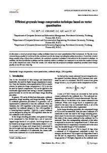
The subsequent two sections, 3.1 and 3.2 describe the framework of our system that is based on quadtree and where q j (t) is an interpolated point between control points p j and p j+1 at parameter value t. To generate parametric line. n points between p j and p j+1 inclusive, the parameter t 3.1 Quadtree is divided into n − 1 intervals between 0 and 1 inclusive Quadtree is a data structure that is widely used for such that q j (0) = p j and q j (1) = p j+1 . In order to represent the non-homogeneous quadimage storage, representation and processing [2, 9]. Quadtree is most often used to partition a 2-D space by rants, we scanned the image data row wise and fitted recursively subdividing it into four quadrants or blocks the parametric line to pixels of non-homogeneous quaduntil each quadrant contains only pixels of one color or rants. Parametric line fitting helps to further reduce the luminance. Recursively subdividing may result a quad- data size in two ways. First, the parametric line fitrant that contains only single pixel. This conventional ting helps to represent the pixels of one color/luminance

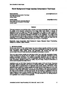
Figure 1: Original image of size 509 × 486. The image Figure 2: The image of Fig. 1 is padded. Size of the padded image is 512 × 512. Padded area on right and size is not a power of 2. bottom is shown in black color. with smaller data set. Second, the parametric line fitting merges the data of a row, belong to more than one shows padded image, where padded area is shown non-homogeneous quadrant, as a single data set. This in black color (internally image matrix has -1 value single merged row removes the artificial boundaries befor padded area). Let J is the padded image of size, tween quadrants that have been imposed by quadtree w × h . For example, if size of I is 509 × 486 then decomposition. It is very likely that at the boundaries of after padding, the size of J would be 512 × 512. two adjacent non-homogeneous quadrants, pixels have 2. Specify threshold of minimum block size Blmt for same luminance. By merging quadrants, large number quadtree decomposition. For example when Blmt = of pixels can be represented by small output data ob4, the minimum block size would be 4 × 4. tained from parametric line fitting. This also solves the 3. Apply the quadtree decomposition to image J. second drawback of conventional quadtree representaThis yields homogeneous quadrants and nontion of image, as described in the previous section 3.1. homogeneous quadrants. Figure 3 shows homogeneous and non-homogeneous quadrants of a 4 Algorithm quadtree decomposed image, minimum block size is This section presents the details of our algorithm for 4 × 4. Non-homogeneous quadrants have pixels of image compression. The encoding part of the algorithm more than one luminance value; therefore it is not consists of two main phases. The first phase consists of worth to save each pixel (total 16 pixels in a miniquadtree decomposition and the second phase consists mum size quadrant) of non-homogeneous quadrants of parametric line fitting. The decoding is relatively a individually. simple process and we described it in a single phase. 4. Entropy encode the data of homogeneous quadrants Let we have a gray-scale image I of size w × h, as (blocks). Each homogeneous quadrants is identified shown in Fig. 1. Let pi, j is luminance of a pixel at by, (i) size of the quadrant, because width and height spatial location (i, j), where 0 ≤ pi, j ≤ 255, 1 ≤ i ≤ h of a quadrant are always equal, therefore only single and 1 ≤ j ≤ w. value is required to save, (ii) (x, y) coordinates of upper left corner of the quadrant, (iii) luminance of the 4.1 Encoding quadrant. There are multiple quadrants of same size, 4.1.1 Phase 1: Quadtree Encoding therefore for efficient storage, we created a list of 1. If size of image I is not a power of 2 then pad the sizes and each element of list has reference towards right and bottom borders of I with -1’s. The Fig 2 (ii) and (iii) of all quadrants whose size is equal to

corresponding element in the list. There is no need to save the data of any quadrant in J which is completely outside of original image I. It can easily be determined by comparing the upper left corner coordinates of a quadrant with the value of w and h. 5. Replace the luminance values of pixels of homogeneous quadrants in J with -1. In Fig. 4 we showed homogeneous quadrants with green color, while non-homogeneous quadrants are shown with their actual luminance value. Let the K is the image we obtained after replacing pixels of homogeneous quadrants in J with -1. 4.1.2

Phase 2: Parametric Line Encoding

1. Specify threshold of fitting λ lmt . The value of λ lmt is 0 for lossless fitting (compression), while λ lmt > 0 for lossy compression. 2. Scan the pixels of image K row by row. During scanFigure 3: A quadtree decomposed image; minimum ning skip the pixels of values -1. In other words, we block size is 4 × 4. Boundaries of homogeneous and are skipping the pixels of homogeneous quadrants, non-homogeneous quadrants are shown with blue and because they are already represented by quadtree. red colors respectively. Let Ri is the set of pixels in the ith row of image K. Let Ri is the set of pixels in the ith row of image K, excluding pixels of value -1, |Ri | ≤ |Ri | 1 . 3. Apply the fitting process to pixel values of each row of image K separately as follows:

Figure 4: A quadtree decomposed image, minimum block size is 4 × 4. Homogeneous quadrants are filled with -1, shown in green color. Non-homogeneous quadrants are shown with their actual luminance values.

(a) Ri = {pi,1 , pi,2 , . . . , pi,n } consists of luminance values of all pixels in ith row (excluding pixels of homogeneous quadrants). Each element in Ri can be considered as a point in 1-dimensional Euclidean space. We call the set points in Ri as original data. (b) Take the first and the of Ri as break last pixels points, i.e., BP = p(i,1) , p(i,n) . For example, BP = p(i,1) , p(i,105) , assuming there are 105 pixels in the ith row, excluding pixels of -1 value. A segment (c) Divide the Ri into segments. is a set of all points (pixels) between two adjacent breakpoints. There is only one segment in the first iteration between p(i,1) and p(i,n) , but when new breakpoints would be added in the following iterations then the number of segments would be increased. For example, suppose there are four break points, i.e., BP = p(i,1) , p(i,55) , p(i,75) , p(i,105) . Then there would be three segments, S1 = 1 |A|

denotes cardinality of set A

(e)

(f) (g)

(h)

(i)

Luminance

Luminance

(d)

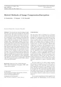
p(i,1) , . . . , p(i,55) , S2 = p(i,55) , . . . , p(i,75) , also suitable for lossy coding and yields higher compression (less number of breakpoints gives and S3 = p(i,75) , . . . , p(i,105) . higher compression) with very little distortion. Apply the fitting process to each segment by taking each pair of adjacent breakpoints as the 300 first and the last point of parametric line and obtain the fitted data by Eq. 1. Number of seg250 ments and number of points in the fitted data are equal to number of segments and number 200 of points in the original data respectively. Let Qi is the set of points in the fitted data, then 150 Qi = {qi,1 , qi,2 , . . . , qi,n }. Compute the squared distance for each point be100 2 tween Ri and Qi i.e., d 2j = p(i, j) − q(i, j) , 1 ≤ j ≤ n. 50 Original Data Fitted Data Find λ max = Max d12 , d22 , . . . , dn2 , λ max ∈ kth Breakpoints segment. 0 1 10 20 30 If λ max > λ lmt then replace the kth segment x−coordinates of scan row of image by two new segments at the point where the squared distance is maximum. For exFigure 5: Fitting with 2 breakpoints. 2 , it means that squared ample, if λ max =d37 distance between p(i,37) and q(i,37) is max300 imum. Since p(i,37) is in segment S1 = p(i,1) , . . . , p(i,55) , , therefore split S1 at p(i,37) 250 and replace S1 by S1a = p(i,1) , . . . , p(i,37) and S1b = p(i,37) , . . . , p(i,55) . 200 Add a new breakpoint bpnew in the set of 150 breakpoints, i.e., BP = {BP} {bpnew }. For example, if before spitting, 100 BP = p(i,1) , p(i,55) , p(i,75) , p(i,105) and bpnew =p(i,37) then after splitting, 50 BP = p(i,1) , p(i,37) , p(i,55) , p(i,75) , p(i,105) . Original Data Fitted Data Go to step 3c and repeat the fitting process with Breakpoints max 0 bethe new set of breakpoints, until the λ 1 10 20 30 x−coordinates of scan row of image tween any two points of original and fitted data is less than or equal to λ lmt . Figures 5 - 11 Figure 6: Fitting with 3 breakpoints. show how the fitting process works for a row of image data. Pixels belong to third row of a (j) Entropy encode the final set of breakpoints image are scanned, while pixels belong to ho(BP) and count of interpolation points (C) mogeneous quadrants are skipped (because they between breakpoints. This is required are already represented by quadtree). Then parato decode the spline fitted data. For exmetric line is fitted to pixel values. Initially first ample, if the final set of breakpoints is, and last pixels are taken as breakpoints. Due to , then , p , p , p , p BP = p (i,1) (i,37) (i,55) (i,75) (i,105) break-and-fit strategy other pixels are added as count of interpolating points would be: C= new breakpoints during fitting process. Even{37 − 1 + 1, 55 − 37 + 1, 75 − 55 + 1, 105 − 75 + 1}, tually all data is fitted with 0 error (lossless {37, i.e., C = 19, 21, 31}. coding) with very few breakpoints. It is also worth to note that by using only 3 breakpoints, 4.2 Decoding as shown in Figure 6, sufficient fitting accuracy 1. Create an empty image (all pixels of 0 values) L of is achieved. This implies that the method is size w × h . The size of L is equal to the padded

300

300

250

250

200 Luminance

Luminance

200

150

100

100

50

50

0

150

Original Data Fitted Data Breakpoints 1

10 20 x−coordinates of scan row of image

0 30



30

Figure 10: Fitting with 7 breakpoints.

Figure 7: Fitting with 4 breakpoints. 300 300 250 250 200 Luminance

Luminance

200

150

150

100 100 50 50

0



0 30

300

250

Luminance

200

150

100

0




1


30



50

Original Data Fitted Data Breakpoints

30

image J. 2. Assign -1 value to each pixel of homogeneous quadrants of L. We know the coordinates of homogeneous quadrants, because we saved the size and the coordinates of homogeneous quadrants during step 4 of quadtree encoding process. 3. Using BP and C, obtained in the step 3j of parametric line encoding process, perform the parametric line interpolation. This yields the parametric line data Q pl . 4. Fill L with Q pl with skipping pixels of -1 value. In other words we are skipping homogeneous quadrants. This yields portion of image decoded by parametric line. 5. Fill the homogeneous quadrants of L using actual values of homogeneous quadrants. We saved the val-

ues of each block of homogeneous quadrants in step 4 of encoding process, besides its size and coordinates. 6. Trim L to size w × h, i.e,. equal to the size of the original image I. This is the decoded image. 5

Experiments and Results

We tested our method on various types of synthetic images such as clip-art, animation, cartoon, medical image, scientific plot, wavelet transformed, etc. Table 1 gives the details of input images. All input images are bitmap images, with 256 possible gray-levels (0-255), stored at 8 bit per pixel. Figure 1, and Figures 12 17 show input images. Images are scaled to fit on paper. In figures with white background, rectangle boxes are drawn around images to visualize boundaries of images. Table 2 shows the bit-rate performance of GIF, PNG and our method (QPL). From Table 2 it is evident that the QPL preformed better than GIF and PNG for all images except for Text image, where PNG performs slightly better. The good performance of QPL is due to the fact that in the first phase, it exploits both horizontal and vertical redundancy using quadtree structure. GIF and PNG do not exploit horizontal and vertical redundancy simultaneously. In the second phase, QPL further reduces the redundancy of those pixels showing constant or linear luminance variation by parametric line fitting. By imposing minimum block size constraint our quadtree decomposition does not fall in the trap of very small blocks.

Figure 12: Play, a cartoon image.

Table 1: Details of input images used in the simulation. Image Name Planter Play Text Style Bone Wavelet Meshgrid

6

Type Clip-art Cartoon Text Computer Animation Medical (X-ray) Wavelet transform Scientific plot

w×h 509 × 486 420 × 315 704 × 395 250 × 314 560 × 420 400 × 352 560 × 420

Discussion

Encoding/Decoding of RGB image: We described the algorithm for gray-scale image. To apply the algorithm on true color or RGB or HSV image, each dimension Figure 13: Text, a text image. Original image is rotated (channel) is processed separately. Lossless and Lossy Compression: The proposed 90 degree counter-clockwise.

Table 2: Bitrate (bit per pixel, bpp) performance of GIF, PNG and QPL for lossless compression. For QPL minimum block size is 4 × 4. Image Name Planter Play Text Style Bone Wavelet Meshgrid

bpp (GIF) 0.6633 1.5689 1.7398 0.8728 0.5452 0.3891 0.3866

bpp (PNG) 0.7965 1.5618 1.5150 1.0517 0.5113 0.4497 0.4215

bpp (QPL) 0.6180 1.3497 1.5220 0.8204 0.4389 0.3587 0.3349 Figure 15: Meshgrid, a scientific plot.

Figure 16: Bone, a medical (x-ray) image.

Figure 14: Style, an animation image.

method can be used for both lossless and lossy compression, while both GIF and PNG are inherently lossless compression schemes and cannot be used for lossy compression. In our method, the only difference between lossless and lossy compression is the value of parameter λ lmt , i.e., threshold of fitting. The value of λ lmt is zero for lossless compression, while λ lmt is greater than zero for lossy compression. Using higher degree Bézier curves: Parametric line is

Figure 17: Wavelet, a wavelet transform image.

a linear Bézier curve. Mathematical model of parametric line (linear Bézier) is analogous to higher degree Bézier curves such as quadratic or cubic Bézier curves. After experiments, we found that parametric line is more suitable than higher degree Bézier curves; both from compression and computational perspectives. Fitting by any form of straight line e.g., polyline [1, 6] would yield the same results as parametric line. 7

Conclusion

We presented a new hybrid scheme for image data compression using quadtree decomposition and parametric line fitting. We described the encoding and decoding steps of algorithm. The encoding composed of two main phases. In the first phase, the method finds the homogeneous and non-homogeneous quadrants using quadtree decomposition with constraint of minimum block size. Homogeneous quadrants are represented by quadtree. In the second phase, the method fits the parametric line to non-homogeneous pixels of each row. Experimental results show that the proposed scheme performs better than well-known lossless image compression techniques for several types of synthetic images. Acknowledgement We are thankful to Keio Leading-edge Laboratory (KLL) of Science and Technology for research grant to doctorate students for the year 2005-06 and 2006-07. References [1] Boris Aranov, Tetsuo Asano, Naoki Katoh, Kurt Mehlhorn, and Takeshi Tokuyama. Polyline fitting of planar points under min-sum criteria. In Algorithms and Computation: 15th International Symposium, ISAAC 2004, volume 3341 of Lecture Notes in Computer Science, pages 77–88, HongKong, China, December 2004. Springer. [2] Sarah F. Frisken and Ron Perry. Simple and efficient traversal methods for quadtrees and octrees. Journal of Graphics Tools, 7(3):1–11, 2002. [3] http://www.w3.org/Graphics/GIF/spec-gif89a.txt. [4] J.M. Gilbert and R.W. Brodersen. A lossless 2-d image compression technique for synthetic discrete-tone images. Data Compression Conference, 1998. DCC ’98. Proceedings, page 0359, 1998. [5] John Miano. Compressed image file formats: JPEG, PNG, GIF, XBM, BMP. ACM Press/Addison-Wesley Publishing Co., New York, NY, USA, 1999. [6] Joseph O’Rourke. An on-line algorithm for fitting straight lines between data ranges. Communications of the ACM, 24(9):574–578, 1981.

[7] http://www.libpng.org/pub/png/. [8] RFC. Deflate compressed data format specification version 1.3. http://tools.ietf.org/html/rfc1951. [9] Hanan Samet. Data structures for quadtree approximation and compression. Communications of the ACM, 28(9):973–993, 1985. [10] Khalid Sayood. Introduction to Data Compression. Morgan Kaufmann, third edition, 2005. [11] Yi-Chen Tsai, Ming-Sui Lee, Meiyin Shen, and C.C. Jay Kuo. A quad-tree decomposition approach to cartoon image compression. IEEE 8th Workshop on Multimedia Signal Processing, 17(6):456–460, October 2006. [12] Terry A. Welch. A technique for high-performance data compression. IEEE Computer, 17(6):8–19, 1984. [13] http://en.wikipedia.org/wiki/GIF. [14] http://en.wikipedia.org/wiki/Portable Network Graphics. [15] Jacob Ziv and Abraham Lempel. A universal algorithm for sequential data compression. IEEE Transactions on Information Theory, 23(3):337–343, 1977.