Jun 13, 2017 - {1, 2,...,q}, Qi = Lâ²i(LiLâ²i)â1, and. ¯zi(k â 1) = â sâNi(Ïk) zs(k â 1). ..... [4] T. Kim, H. Shim, and D. D. Cho. Distributed luenberger observer.
A Hybrid Observer for a Distributed Linear System with a Changing Neighbor Graph
arXiv:1706.04235v1 [cs.SY] 13 Jun 2017
L. Wang1, A. S. Morse1 , D. Fullmer1 , and J. Liu2
Abstract— A hybrid observer is described for estimating the state of an m > 0 channel, n-dimensional, continuous-time, distributed linear system of the form x˙ = Ax, yi = Ci x, i ∈ {1, 2, . . . , m}. The system’s state x is simultaneously estimated by m agents assuming each agent i senses yi and receives appropriately defined data from each of its current neighbors. Neighbor relations are characterized by a time-varying directed graph N(t) whose vertices correspond to agents and whose arcs depict neighbor relations. Agent i updates its estimate xi of x at “event times” t1 , t2 , . . . using a local observer and a local parameter estimator. The local observer is a continuous time linear system whose input is yi and whose output wi is an asymptotically correct estimate of Li x where Li a matrix with kernel equaling the unobservable space of (Ci , A). The local parameter estimator is a recursive algorithm designed to estimate, prior to each event time tj , a constant parameter pj which satisfies the linear equations wk (tj −τ ) = Lk pj +µk (tj −τ ), k ∈ {1, 2, . . . , m}, where τ is a small positive constant and µk is the state estimation error of local observer k. Agent i accomplishes this by iterating its parameter estimator state zi , q times within the interval [tj − τ, tj ), and by making use of the state of each of its neighbors’ parameter estimators at each iteration. The updated value of xi at event time tj is then xi (tj ) = eAτ zi (q). Subject to the assumptions that (i) none of the Ci are zero, (ii) the neighbor graph N(t) is strongly connected for all time, (iii) the system whose state is to be estimated is jointly observable, (iv) q is sufficiently large and nothing more, it is shown that each estimate xi converges to x exponentially fast as t → ∞ at a rate which can be controlled.
I. I NTRODUCTION In a recent paper [1], a distributed observer was described for estimating the state of an m > 0 channel, n-dimensional, continuous-time, jointly observable linear system of the form x˙ = Ax, yi = Ci x, i ∈ {1, 2, . . . , m}. The state x is simultaneously estimated by m agents assuming each agent i senses yi and receives the state of each of its neighbors’ estimates. This work was supported by National Science Foundation grant n. 1607101.00 and US Air Force grant n. FA9550-16-1-0290. 1 L. Wang, A. S. Morse and D. Fullmer are with the Department of Electrical Engineering, Yale University, New Haven, CT, USA. {lili.wang, as.morse,
daniel.fullmer}@yale.edu 2 J. Liu is with Coordinated Science Laboratory, University of Illinois at Urbana-Champaign, Champaign, IL, USA.
{jiliu}@illinois.edu
An attractive feature of the observer described in [1] is that it is able to generate an asymptotically correct estimate of x at a pre-assigned exponential rate, if each agent’s neighbors do not change with time and the neighbor graph characterizing neighbor relations is strongly connected. However, a shortcoming of this observer is that it is unable to function correctly if the network changes with time. Changing neighbor graphs will typically occur if the agents are mobile. A second shortcoming of the observer described in [1] is that it is “fragile.” By this we mean that the observer is not able to cope with the situation when an agent’s neighbors change. For example, if because of a component failure, a loss of battery power or some other reason, an agent drops out of the network, what remains of the observer will typically not be able to perform correctly and may become unstable, even if what is left is still a jointly observable system with a strongly connected neighbor graph. The aim of this paper is to describe a new type of observer which overcomes these difficulties. II. T HE P ROBLEM We are interested in a network of m > 0 autonomous agents labeled 1, 2, . . . , m which are able to receive information from their neighbors where by the neighbor of agent i is meant any other agent in agent i’s reception range. We write Ni (t) for the set of labels of agent i’s neighbors at real time t ∈ [0, ∞) and we take agent i to be a neighbor of itself. Neighbor relations at time t are characterized by a directed graph N(t) with m vertices and a set of arcs defined so that there is an arc from vertex j to vertex i whenever agent j is a neighbor of agent i. Each agent i can sense a continuous-time signal yi ∈ IRsi , i ∈ m = {1, 2, . . . , m}, where yi x˙
= Ci x, = Ax
i∈m
(1) (2)
and x ∈ IRn . We assume throughout that Ci 6= 0, i ∈ m, and that the system defined by (1), (2) is jointly ′ ′ observable; i.e., with C = [ C1′ C2′ · · · Cm ] , the matrix pair (C, A) is observable. The problem of interest is to develop “private estimators”, one for each agent, which enable each agent to obtain an asymptotically correct estimate of x.
A. Background Distributed state estimation problems have been under study in one form or another for years. In many cases system and measurement noise are components of the problem considered and some form of Kalman filtering is proposed. The literature on this subject is vast, and many specialized results exist; see for example, [2]–[10] and the many references cited therein. However, to the best of our knowledge, the specific problem we have posed has not been solved without imposing restrictive assumptions. One reason for this we think is because most approaches rely on estimators which are timeinvariant linear systems. We believe that the problem posed, involving a time-varying neighbor graph, cannot be solved without qualification, with a time invariant linear system. It would be especially useful to know whether or not this conjecture is true. III. O BSERVER The idea we are about to present makes use of to two familiar types of systems. The first type is a classical observer; such systems enable each agent to generate an asymptotically correct estimate of the “part of x which is observable” to that particular agent. The second type of system is a parameter estimator; using parameter estimators enables each agent to generate an asymptotically correct estimate of x frozen at a specified time instant by viewing x at that time as a fixed parameter. The judicious combination of these two types of systems provides a straightforward, easy to analyze solution to the problem we have posed and it is surprising that the idea has not been suggested before. The observer to be described consists of m estimators, one for each agent. Agent i generates an estimate xi of x with its private estimator Ei which is a hybrid dynamical system consisting of a “local observer” and a “local parameter estimator.” Each xi is updated at event times t1 , t2 , . . . where tj = jT, j ≥ 1, and T is a pre-selected positive real number. Between event times, each xi satisfies x˙ i = Axi . Agent i’s local observer is a continuous time linear system whose input is yi and whose output wi is an asymptotically correct estimate of Li x where Li a matrix with kernel equaling the unobservable space of (Ci , A). The computations needed to update each agent’s estimate of x at event time tj are carried out over the time interval [tj − τ, tj ); here τ is a positive number smaller than T which is chosen large enough so that the computations required to update each agent’s estimate can be completed in τ time units. Agent i’s local parameter estimator is a recursive algorithm designed to estimate on each interval [tj − τ, tj ), a constant parameter pj which satisfies the linear equations wk (tj −τ ) = Lk pj +µk (tj −τ ), k ∈ m,
where µk is the state estimation error of local observer k. Agent i accomplishes this by iterating its parameter estimator state zi , q times within the interval [tj − τ, tj ), and by making use of the state of each of its neighbors’ parameter estimators at each iteration. The updated value of xi at event time tj is then xi (tj ) = eAτ zi (q). A. Estimator Ei In this section we give a more detailed description of agent i’s private estimator. As just stated, the estimator consists of a local observer and a local parameter estimator. 1) Local Observer i: Recall that the unobservable space of (Ci , A), written [Ci |A], is the largest Ainvariant subspace contained in the kernel of Ci . Set ni = n − dim([Ci |A]) and let Li be any ni × n matrix whose kernel is [Ci |A]. Then as is well known, the equations Ci = C¯i Li and Li A = A¯i Li have unique solutions C¯i and A¯i respectively and (C¯i , A¯i ) is an observable matrix pair. By a local observer for agent i is meant any ni dimensional system of the form w˙ i = (A¯i + Ki C¯i )wi − Ki yi
(3)
where Ki is a matrix to be chosen. It is easy to verify ∆ that the local observer estimation error µi = wi − Li x satisfies ¯
¯
µi (t) = e(Ai +Ki Ci )t (wi (0) − Li x(0)),
t ∈ [0, ∞)
Moreover, since (C¯i , A¯i ) is observable, Ki can be selected so that µi (t) converges to 0 exponentially fast at any pre-assigned rate. We assume that each Ki is so chosen. Since wi (t) = Li x(t) + µi (t),
t ∈ [0, ∞)
(4)
wi can be thought of as an asymptotically correct estimate of Li x. 2) Local Parameter Estimator i: The starting point for the development of the local parameter estimators is the observation that for each event time tj , the system of equations wi (tj − τ ) = Li pj + µi (tj − τ ), i ∈ m
(5)
has a unique solution, namely pj = x(tj − τ ). This is a consequence of (4) and the joint observability assumption. It is useful to think of the estimation of pj as a parameter estimation problem. One algorithm for computing pj which would give an asymptotically correct result in an infinite number of steps if each µk (tj − τ ) were zero, is the algorithm described in [11]. In this paper we will make use of this algorithm but will only iterate q > 0 steps where q is an integervalued design constant which is chosen large enough to ensure exponential convergence; we assume that the
local processers are sufficiently fast so that each can execute q iterations in τ time units. The local parameter estimator for agent i as defined as follows. For each event time tj , zi (0) = xi (tj − τ ) zi (k) = z¯i (k − 1)
(6)
−Qi (Li z¯i (k − 1) − wi (tj − τ )), k ∈ q (7) xi (tj ) = eAτ zi (q) (8) ∆
where k ∈ q = {1, 2, . . . , q}, Qi = L′i (Li L′i )−1 , and X zs (k − 1). z¯i (k − 1) = s∈Ni (τk )
Here
� � (k − 1) τ τk = tj − 1 − q
and mi (k) is the number of labels in Ni (τk ). Note that the same symbols zi (k − 1) and τk are used on each interval [tj − τ, tj ), j ≥ 1, without explicitly showing their dependence on j. One way to modify the above algorithm without changing its essential features, is to redefine each Qi in (7) as Qi = L′i Gi where Gi is any positive definite matrix for which the spectrum of L′i Gi Li is contained in the open half interval (−1, 1]. It is known that with this modification, the algorithm has the same convergence properties as the original but perhaps with a faster convergence rate if the Gi are chosen appropriately [11]. IV. M AIN R ESULT The main result of this paper is as follows. Theorem 1: Suppose that (1), (2) is jointly observable, that Ci 6= 0, i ∈ m, and that the neighbor graph N(t) is strongly connected for all t ∈ [0, ∞). Then for appropriately chosen T, τ, q, and Ki , i ∈ m, there exist positive constants g and λ for which the following statement is true. For each initial process state x(0), each initial local observer state wi (0), i ∈ m, and each estimate xi (0), i ∈ m, |xi (t) − x(t)|2 ≤ e−λt (δx + δµ ), t ≥ 0, i ∈ m (9) where δx = max |xi (0)−x(0)|2 , δµ = g max |wi (0)−Li x(0)|2 i∈m
i∈m
and | · |2 is the standard two norm. It is possible to give a formula for λ. Towards this end, assume that q has been chosen large enough so that ζT (10) q > 1 + � � ((m − 1)2 + 1) ln γ1
where ζ is the largest eigenvalue of 21 (A + A′ ), and γ is the positive number defined by (21) in Proposition 1; note that γ is less than 1 and depends only on m and the Li which in turn depend only on A and the Ci . Next let ω be any positive number such that � � r 1 ω + ζ > ln (11) T γ where r is the unique integer quotient of q divided by (m− 1)2 + 1. Assume that the Ki used in the definitions of the local observers, have been chosen so that each local observer estimation error decreases in norm as fast as e−ωt does. A formula for λ is then � � r 1 −ζ (12) λ = ln T γ Note that so long as (10) holds, λ > 0. Note also that the formula for γ in Proposition 1 is conservative and consequently so is the above formula for λ. A. Example The following example illustrates how the observer performs when applied to an unstable system. Consider the three channel, four-dimensional, continuous-time system described by the equations x˙ = Ax, yi = Ci x, i ∈ {1, 2, 3}, where
0 0 A= 0 0
0.4 0 0 0 0 0 0 0 2 0 −2 0.2
C1
=
[1 0
0 0]
C2
=
[0 1
0 0]
C3
=
[0 0
1 1]
Note that A has two eigenvalues at 0 and a pair of complex eigenvalues at 0.1 ± j2.00. While the system is jointly observable, no single pair (Ci , A) is observable. For this example N1 = {1, 2}, N2 = {1, 2, 3}, N3 = {2, 3}, T = 1, τ = 0.5, γ = 0.975 and ζ = 0.2. To satisfy (10), q is chosen as q = 45 and r = 9. To satisfy (11), ω is chosen as ω = 2. The local observers for the three agents are constructed using the following matrices. For agent 1: � � 0 0 C¯1 = [ 0 1 ] , A¯1 = , 0.4 0 � � � � 0 1 0 0 20 L1 = , K1 = − 1 0 0 0 6
For agent 2: C¯2 = 1, A¯2 = 0, L2 = [ 0 1 For agent 3:
0 0 ] , K2 = −2
� � √ 0.1 −1.9 , 2 ] , A¯3 = C¯3 = [ 0 2.1 0.1 √ √ � � � � 0 0 −√ 22 √22 0.85 L3 = , K = − 3 2 2 3.68 0 0 2 2
10 x(3)
x(3) , x(3) 1
5
(3)
x1
0 -5 -10 0
1
2
3
4
5
3
4
5
(a)
t
6
5 0
x(3) -x(3) 1
In all three cases the convergence rate is 2. Finally, for this example (12) gives an overall convergence rate of λ = 0.025. This system was simulated with x(0) = [ 3 2 4 1 ]′ as the initial state of the process, ′ ′ w1 (0) = [ 2 4 ] , w2 (0) = [ 3 ], and w3 (0) = [ 1 2 ] as the initial states of the three local observers, and x1 (0) = x2 (0) = x3 (0) = − [ 4 4 4 4 ]′ as the initial estimates of the three local estimators. The two traces in Figure 1a show the simulation result for the third components of x1 and x respectively, namely (3) x1 and x(3) . The trace in Figure 1b shows the error (3) x1 − x(3) while the trace in Figure 1c, shows the two-norm of the error x1 − x.
-5 -10 -15 0
1
2
6
20 10
|x 1-x|2
x(3) , x(3) 1
(b)
15
x(3) (3) x1
5 0
t
10 5
-5
0 0
-10 0
1
2
3
4
5
(a)
t
1
2
3
4
5
(c)
6
t
6
5
Fig. 2.
Simulation Results with System Noise
x(3) -x(3) 1
0 -5 -10 0
1
2
3
4
5
t
6
ǫi (0) =
(b)
20
ǫi (k) =
15
|x 1-x|2
denote the parameter estimation error ǫi (k) = zi (k) − pj , k ∈ {0, 1, . . . , q}. We claim that eA(T −τ ) (xi (tj−1 ) − x(tj−1 )) (13) X 1 ǫs (k − 1) Pi mi (k) s∈Ni (τk )
10 5
xi (tj ) − x(tj ) =
0 0
1
2
3
4
(c)
Fig. 1.
5
t
6
Simulation Results
To study the effect of an unmeasured disturbance driving the process dynamics, a second simulation was performed using the same observer as above applied to the modified state equation system x˙ = Ax + bν where b = [ 1 1 1 1 ]′ and ν = 7 cos 10t. The resulting traces are shown in Figures 2a, 2b, and 2c respectively. V. A NALYSIS Fix j > 0. Our immediate aim is to analyze the behavior of the parameter estimators on the time interval [tj − τ, tj ) . Towards this end, for each i ∈ m let ǫi
+Qi µi (tj − τ ), eAτ ǫi (q)
k∈q
(14)
(15)
where t0 = 0, and Pi is the orthogonal projection matrix Pi = I − L′i (Li L′i )−1 Li . To establish (13), note that ǫi (0) = xi (tj − τ ) − x(tj − τ ) because of (6), the definition of ǫi and the fact that pj = x(tj − τ ); (13) follows at once. The recursion in (14) is an immediate consequence of (5) and (7). To establish (15), note that xi (tj ) − x(tj ) = eAτ zi (q) − x(tj ) because of (8); but x(tj ) = eAτ x(tj − τ ) = eAτ pj . Therefore (15) is true. ′ To proceed define x b = [ x′1 x′2 · · · x′m ] , x ¯ = ′ ′ ′ ′ ′ ′ ′ ′ [ x x · · · x ] and ǫ = [ ǫ1 ǫ2 · · · ǫm ] . Write Fj (k) for the “flocking matrix” determined by N(τk ); −1 i.e., Fj (k) = DN(τ A′N(τk ) where DN(τk ) is the diagonal k) matrix of in-degrees of the vertices of N(τk ) and AN(τk ) is the adjacency matrix of N(τk ). Then it is easy to verify that ǫ(0) =
¯
eA(T −τ ) (b x(tj−1 ) − x ¯(tj−1 ))
ǫ(k) = x b(tj ) − x¯(tj ) =
P (Fj (k) ⊗ I)ǫ(k − 1) +Qµ(tj − τ ), k ∈ q ¯
eAτ ǫ(q)
′
where µ = [ µ′1 µ′2 · · · µ′m ] , A¯ = block diagonal{A, A, ..., A}, P = block diagonal{P1 , P2 , ..., Pm }, Q = block diagonal{Q1 , Q2 , . . . , Qm }, ⊗ is the Kronecker product, and I is the n × n identity matrix. From these equations it follows that x b(tj ) − x ¯(tj ) = Ωj (b x(tj−1 ) − x¯(tj−1 )) + Θj µ(tj − τ ) (16) where Ωj
=
¯
eAτ P (Fj (q) ⊗ I)
¯
P(Fj (q−1)⊗I)· · ·P(Fj (1)⊗I)eA(T−τ ) (17) and ¯
Θj = eAτ ! q X P(Fj (q)⊗I)P(Fj (q−1)⊗I)· · ·P(Fj (s)⊗I)+I Q(18) s=2
Suppose that with some suitably defined norm, the norm of each Ωj is less than one and Θj is uniformly bounded as a function of j. Then the sequence x b(tj )−¯ x(tj ), j ≥ 1 will converge to zero at a exponential rate, because the sequence µj (tj − τ ), j ≥ 1 converges to zero at an exponential rate. Because of this and the fact that the time between successive event times is T , x b(t) will converge to x ¯(t) exponentially fast. In view of the definitions of x b and x ¯, it is obvious that each xi will converge to x exponentially fast. So establishing convergence boils down to establishing the aforementioned properties of the Ωj and Θj sequences. For this a suitably defined matrix norm is needed. Such a norm, termed a mixed-matrix norm,” has been defined before [12] and is described below. Let | · |∞ denote the standard induced infinity norm and write IRmn×mn for the vector space of all m × m block matrices M = [ Mij ] whose ijth entry is a matrix Mij ∈ IRn×n . As in [12] we define the mixed matrix norm of M ∈ IRmn×mn , written ||M ||, to be ||M || = |hM i|∞
(19)
where hM i is the matrix in IRm×m whose ijth entry is |Mij |2 . It is very easy to verify that || · || is in fact a norm. It is even sub-multiplicative [12]. Corollary 1 of [12] and its proof imply the following. Proposition 1: Let P1 , P2 , . . . , Pm be any set of n×n orthogonal matrices for which ∩i∈m ker Pi = 0. Let N1 , N2 , · · · , N(m−1)2 be any sequence of selfarced, strongly connected, directed graphs on m vertices; for i ∈ m, write Fi for the flocking matrix Fi =
Di−1 A′i where Di is the diagonal matrix of in-degrees of vertices of Ni and Ai is the adjacency matrix of Ni . Let C denote the compact set of products of form Pj1 , Pj2 , · · · , Pj(m−1)2 where each of the Pi , i ∈ m, occurs in the product at least once. Then, ||P (F(m−1)2 ⊗I)P (F(m−1)2 −1 ⊗I) · · · P (F1 ⊗I)P || ≤ γ (20) where (m − 1)(1 − ρ) γ =1− (21) m(m−1)2 and ρ = max |Pj1 Pj2 · · · Pj(m−1)2 |2 . Moreover, ρ < 1 C and γ < 1. With Proposition 1, the following property of the Ωj sequence can be derived. Lemma 1: Let ζ be the largest eigenvalue of matrix 1 (A + A′ ). Suppose that q > (m − 1)2 + 1 and that 2 N(t) is a self-arced, strongly connected neighbor graph for all t ≥ 0. Then kΩj k ≤ eζT γ r where r is the unique integer quotient of q divided by (m − 1)2 + 1. Proof of Lemma 1: Since N(t) is strongly connected for all time, within each time interval [tj − τ, tj ), the graphs of the sequence N(τ1 ), N(τ2 ), . . . , N(τq ) are all strongly connected. Also the graphs of the sequence are all self-arced. By Proposition 1 and sub-multiplicativity of the mixed-matrix norm, kP (Fj ((m − 1)2 + c + 1) ⊗ I)
P (Fj ((m + 1)2 + c) ⊗ I) · · · P (Fi (c) ⊗ I)k ≤ γ
for any positive integer c. Thus we have kP (Fj (q) ⊗ I)P (Fj (q − 1) ⊗ I) At
· · · P (Fj (1) ⊗ I)k ≤ γ r
By [13], we know |e |2 ≤ e
ζt
(22)
which means
¯ At
ke k = |eAt |2 ≤ eζt
(23)
By combining (22) and (23), we get kΩi k
≤ eζτ γ r eζ(T −τ ) ≤ eζT γ r
which completes the proof. Now, with Lemma 1, convergence from xˆ to x ¯ can be derived. Proof of Theorem 1: As a first step, we find the constraint for q such that kΩj k < 1. By Lemma 1, ∆ kΩj k ≤ eζT γ r = β where ζ is the largest eigenvalue of 21 (A + A′ ). It is sufficient to ensure β < 1. Thus we get that if q holds for (10), β < 1 holds. If all the eigenvalue of A is negative, the right hand side of the above inequality is less than zero and it is trivial to set q = 0. Second, since µ(t) converges to zero at a pre-assigned rate, let kµ(t)k ≤ ¯kµ(0)kg1 e−wt where w can be any
positive numbers, and g¯1 is a positive constant. That τ is equivalent to kµ(tj − τ )k ≤ kµ(0)kg1 α T +j , where −wT α=e and g1 is positive. Choose w such that α < β. From (16), we get x ˆ(tj ) − x¯(tj ) =
Ωj Ωj−1 · · · Ω1 (ˆ x(0) − x ¯(0)) +
j X s=1
∆
Ωj Ωj−1 · · · Ωs+1 Θs µ(ts − τ )
Let g2 = maxs kΘs k. Then kˆ x(tj ) − x ¯(tj )k
≤ kˆ x(0) − x ¯(0)kkΩj Ωj−1 · · · Ω1 k j X T +kµ(0)kg1 g2 kΩj Ωj−1 · · · Ωs+1 kα τ +s s=1
≤ kˆ x(0) − x¯(0)kβ j + kµ(0)kg1 g2
j X
T
β j−s α τ +s
s=1 � � T +τ g1 g2 = kˆ x(0) − x ¯(0)k + kµ(0)k α τ βj β−α g1 g2 T +τ j −kµ(0)k α τ α β−α � � g1 g2 T +τ τ βj α ≤ kˆ x(0) − x ¯(0)k + kµ(0)k β−α
Since β < 1, all xi (tj ) will converge to the real state x(tj ) exponentially fast whose rate is bounded by β. Thus we can get the result that |xi (t) − x(t)|2 ≤ e−λt (σx + σµ ), t ≥ 0, i ∈ m where σx = kˆ x(0) − x ¯(0)k, σµ = kµ(0)k
g1 g2 T +τ α τ β−α
and λ = − T1 ln β which is equivalent to (12). Note kµ(0)k = max |wi (0) − Li x(0)|2 , and i∈m
∆
g=
g1 g2 T +τ α τ β−α
is a positive constant which completes the proof. VI. C ONCLUDING R EMARKS One of the nice properties of the hybrid observer discussed in this paper is that it is resilient. By this we mean that under appropriate conditions it will be able to continue to provide asymptotically correct estimates of x, even if one of the agents leave the network. To give an example of this, suppose that N(t) is a constant, strongly connected, self-arced four vertex graph N with arcs in both directions between each pair of vertices except for the vertex pair (1, 4). Then N will remain self-arced and strongly connected after the removal of any one vertex v and all arcs either leaving or arriving at v. Suppose the system whose state is to be estimated is a jointly observable four channel system which remains jointly
observable after any one measurement yi is removed. Suppose that agent k leaves the network. It is clear that any properly designed hybrid observer for this system will be able generate asymptotically correct estimates of x not only for all four agents but also for the three which remain after agent k leaves. Further research is needed to more fully understand resilient observers. Generally one would like to choose T “small” to avoid unnecessarily large error overshooting between event times. Meanwhile, since r is the unique integer quotient of q divided by (m − 1)2 + 1, it is obvious from (12) that the larger the number of iterations q on each interval [tj − τ, tj ) the faster the convergence. Two considerations limit the value of q - how fast the parameter estimators can compute and how quickly information can be transmitted across the network. We doubt the former consideration will prove very important in most applications, since digital processers can be quite fast and the computations required are not so taxing. On the other hand, transmission delays will almost certainly limit the choice of q. A model which explicitly takes such delays into account will be presented in another paper. A second practical issue which this paper does not address is the question of synchronization. Like just about all published papers on distributed estimation, this paper implicitly assumes that all agents share a common clock. This is undoubtedly an unrealistic assumption for many applications. The tools to study this type of observer in an asynchronous setting already exist [14] and we anticipate applying them in the future. A third practical issue is that the development in this paper does not take into account measurement noise. On the other hand, the observer provides exponential convergence and this suggests that if noisy measurements are considered, the system the observer’s performance will degrade gracefully with increasing noise levels. Of course one would like an “optimal” estimator for such situations in the spirit of a Kalman filter. Just how to formulate and solve such a problem is a significant issue for further research. R EFERENCES [1] L. Wang and A. Morse. A distributed observer for a timeinvariant linear system. IEEE Transactions on Automatic Control, 2017. conditionally accepted. [2] S. Park and N. C. Martins. Design of distributed lti observers for state omniscience. IEEE Transactions on Automatic Control, 62(2):561–576, Feb 2017. [3] U. A. Khan and A. Jadbabaie. On the stability and optimality of distributed kalman filters with finite-time data fusion. In Proceedings of the 2011 American Control Conference, pages 3405–3410, Jun 2011. [4] T. Kim, H. Shim, and D. D. Cho. Distributed luenberger observer design. In 2016 IEEE 55th Conference on Decision and Control (CDC), pages 6928–6933, Dec 2016.
[5] Aritra Mitra and Shreyas Sundaram. Distributed observers for lti systems. arXiv:1608.01429, 2016. [6] R. Olfati-Reza and J. S. Shamma. Consensus filters for sensor networks and distributed sensor fusion. In Proceedings of the 44th IEEE Conference on Decision and Control, pages 512–520, 2005. [7] R. Carli, F. Fagnani, A. Speranzon, and S. Zampieri. Communication constraints in the average consensus problem. Automatica, pages 671–684, 2008. [8] L. Xiao, S. Boyd, and S. Lall. A scheme for robust distributed sensor fusion based on average consensus. In Proc. Fourth International Symposium on Information Processiing in Sensor Networks, pages 63–70, 2005. [9] R. Olfati-Reza. Kalman-consensus filter: Optimality, stability, and performance. In Proceedings of the 48h IEEE Conference on Decision and Control (CDC) held jointly with 2009 28th Chinese Control Conference, pages 7036–7042, 2009. [10] F. Dorfler, F. Pasqualetti, and F. Bullo. Continuous-time distributed observers with discrete communication. IEEE Journal of Selected Topics in Signal Processing, 7(2):296–304, 2013. [11] L. Wang, D. Fullmer, and A. S. Morse. A distributed algorithm with an arbitrary initialization for solving a linear algebraic equation. In 2016 American Control Conference (ACC), pages 1078–1081, July 2016. [12] S. Mou, J. Liu, and A. S. Morse. A distributed algorithm for solving a linear algebraic equation. IEEE Transactions on Automatic Control, 60(11):2863–2878, Nov 2015. [13] Guang-Da Hu and Mingzhu Liu. The weighted logarithmic matrix norm and bounds of the matrix exponential. Linear Algebra and its Applications, 390:145 – 154, 2004. [14] J. Liu, S. Mou, and A. S. Morse. An asynchronous distributed algorithm for solving linear algebraic equations. IEEE Transactions on Automatic Control, 2016. conditionally accepted.