A Kullback–Leibler Divergence-based Distributionally Robust ... - arXiv

1

A Kullback–Leibler Divergence-based Distributionally Robust Optimization Model for Heat Pump Day-ahead Operational Schedule in Distribution Networks Zihao Li, Wenchuan Wu, Senior Member, IEEE, Boming Zhang, Fellow, IEEE

Abstract—For its high coefficient of performance and zero local emissions, the heat pump (HP) has recently become popular in North Europe and China. However, the integration of HPs may aggravate the daily peak-valley gap in distribution networks significantly. In this paper, we describe a distributionally robust optimization (DRO)-based heat pump day-ahead operational schedule model (HP-DOSM) to shave the peak and reduce residents’ costs under time-of-use. The ambiguity set of the DRO is constructed using Kullback–Leibler divergence with a nominal distribution. This model can well capture the uncertainties of weather, photovoltaic, and load prediction errors. Moreover, this DRO based HP-DOSM can be transformed into a tractable deterministic model. Compared with robust optimization (RO) models, our model is less conservative since more statistical information of the uncertainties is utilized. Numerical tests were conducted to demonstrate its performance, compared with the RO model via Monte Carlo simulations.

Ck Rw, k Cw, k

xk ,t xk

PHP , k

 COP , k

 w2h,k Z PLoad , k ,t PPV , k ,t Z Ptrans ,t

 P ,t T , t Pt t P0t

1Index

Terms—Distribution network, distributionally robust optimization, day-ahead operational schedule, Kullback–Leibler divergence

Qt

NOMENCLATURE

t

Qt Q0t

N H Tk ,t

Tw, k ,t Tout ,t

Tk Tw, k

Tout Tk

Tk Rk

Total number of houses equipped with heat pump and water tank Time horizon in 1 day Indoor air temperature of the kth house at time t Tank water temperature of the kth house at time t Outdoor temperature at time t Vector

Tk ,0 Tk ,1

T T Vector  w, k ,0 w, k ,1 Tout ,0 Tout ,1

Vector

Tk , H 

T

Tw, k , H  Tout , H 

T

T

Upper temperature boundary of the kth house Lower temperature boundary of the kth house Thermal resistance of the kth house

Manuscript received XXX, 2017. This work was supported in part by the National Science Foundation of China (51477083), in part by Key Science and Technology Project of State Grid Corporation of China (Grant. 5202011600U4). The authors are with the State Key Laboratory of Power Systems, Department of Electrical Engineering, Tsinghua University, Beijing 100084, China (e-mail: [email protected]).

t

Thermal capacitor of the kth house Thermal resistance of the kth water tank Thermal capacitor of the kth water tank ON/OFF (1/0) state of the kth heat pump x x Vector  k ,0 k ,1

xk , H 

T

Rated power of the kth heat pump Coefficient of performance of the kth HP Water tank to house heating efficiency of the kth house Zone of local transformer and feeder lines Load of the kth house except heat pump at time t Photovoltaic power of the kth house at time t Transformer power of zone Z at time t Forecast errors of power at time t Forecast errors of outdoor temperature at time t Distribution of power forecast error at time t P Ambiguity set of t  Center/nominal distribution of t Distribution of outdoor temperature forecast error at time t Q Ambiguity set of t Q Center/nominal distribution of t Farthest KL divergence in the ambiguity set of power forecast error at time t Farthest KL divergence in the ambiguity set of outdoor temperature forecast error at time t I.

INTRODUCTION

(HPs) have seen a revival in recent years, in Heatwhichpumps their potential role with renewable energy sources is being investigated. HP technologies have experienced great improvements in operating stability and have subzero coefficient of performance [1], providing confidence for consumers in their reliability. Unsurprisingly, more than 750,000 units were sold in the EU-20, reducing greenhouse gas emissions by 6.8 Mt in 2010 [2]. However, HPs have placed a considerable load on power systems, although recognized as a promising resource for demand-side management in using renewable energy [3]. In recent years, a policy named ‘Coal to Electricity’ has been promulgated in Beijing, to replace coal stoves in the nearby countryside with HPs for heating, which may be beneficial in reducing the gray smog sky over Beijing [4]. By the end of November 2016,

2 227,000 houses in 663 counties in Beijing had had electrical heaters installed [5]. However, the local distribution networks take the risk of having insufficient capacity in transformers and branches, where more investment in infrastructure is needed. An optimal day-ahead operational schedule strategy for HPs may provide the benefit of peak-shaving [6] and make better use of renewable energy [7]. For a local distribution network, integrated with renewable energy generators and HPs, its day-ahead operational schedule suffers uncertainties, from, for example, weather predictions, load predictions, and renewable energy predictions. Conventionally, stochastic optimization (SO) and robust optimization (RO) techniques have been used to capture uncertainties. Recently, distributionally robust optimization (DRO) has been considered a more practical paradigm for decision making under uncertainty, where the uncertain variable is governed by a probability distribution type that is itself subject to uncertainty [8]. DRO provides more robustness with ambiguous distribution sets and is less conservative than classical RO; moreover, it does not require explicit distribution of uncertain variables, like SO, and demonstrates application potential in many areas [9-12]. The ambiguity set of a DRO problem is a family of distributions, characterized through certain known properties of the real distribution [13] and must be rich enough to include the real distribution while small enough to exclude pathological distributions [14]. How the ambiguity set is constructed is key to DRO, and there are two main ways: moments-based and distance-based methods. The momentsbased method usually defines an ambiguity set by restricting the mean and covariance matrix of the distributions to some given values; thus, the DRO model can be further transformed into a deterministic Semidefinite Programming(SDP) or Second Order Programming(SOCP) problem under several linear assumptions and approximations [12, 15, 16]; however, odd distributions and mixed integer problems may introduce additional complexity. Distance-based methods define the ambiguity set as a ball in the measured space of probability distributions, using a probability distance function, such as the Prokhorov metric [17], Kullback–Leibler divergence (KL divergence) [15, 18], or the Wasserstein metric [14]. Distance-based ambiguity sets limits on the shape of distributions that explicitly use data distribution information and may decrease the conservatism and the robustness that could be controlled with explicit meanings. Due to the ON/OFF nature of HPs, the day-ahead HP operational schedule is a mixed-integer linear program (MILP) with uncertain variables. For moments-based DRO models, methods such as Benders decomposition [19], linear approximation [11], and conic programming methods [20], are used to solve them. However, if these models incorporate mixed-integer variables, they may become intractable. In this paper, a KL distance-based MILP DRO model is described for a HP day-ahead operational schedule. It can be transformed to a tractable deterministic MILP model. Moreover, the distance-based DRO can better use historical data [14, 15, 21]. In [15], it was suggested that adopting distance-based ambiguity sets is less conservative. This paper is based on the works [15, 18], and the major

contributions include the following: (1) A heat pump day-ahead operational schedule model (HP-DOSM) is proposed to shave the peak and reduce residents’ cost, which is formulated as a MILP DRO. A KL divergence-based ambiguity set is used to capture uncertainties in the prediction errors in outdoor temperature, residential load, and photovoltaic power. (2) The proposed MILP DRO model is transformed to a tractable deterministic MILP problem under two nominal distributions: a Gaussian distribution and a kernel density estimator (KDE). (3) Numerical tests show that the proposed approach has potential to provide effective peak shaving and outperforms the conventional RO model. The remainder of the paper is organized as follows. Section II presents the deterministic day-ahead HP operational schedule model. Section III discusses the formulation of MILP DRO model and use of historical data. Numerical tests are described in Section IV. The paper ends with conclusions and future work in Section V. II.

DETERMINISTIC HEAT PUMP DAY-AHEAD OPERATIONAL SCHEDULE MODEL

Figure 1 shows a local distribution network integrated with photovoltaic panels and consumers with air-source HPs. For comfort considerations, the HP first heats the water in a tank to supply heat for the house. The tank is installed indoors and links to a finned tube with constant water flux.

Distribution network

Figure 1. Local distribution network

We apply a one-order equivalent thermal RC model to simulate the house and the water tank. The RC model is Tk  Tw, k formulated as follows, xk  COP , k PHP , k 

Rw, k

 Cw, k Tw, k

T  Tk Tout  Tk   w 2 h , k w, k  CkTk Rk Rw, k

where

Rk , Ck

and

Rw, k , Cw, k

(1) (2)

are the 1st-order thermal

parameters of the house and water tank, respectively, of the k th house, and they can be identified from historical T T T measurements for real application. k , w, k , and out are the indoor air, water tank, and outdoor air temperatures, P   x respectively. HP , k , COP , k , w 2 h , k , and k are the rated power, constant HP to water coefficient of performance (COP), constant water-to-house efficiency, and the ON-OFF

3 kw 2 h , khouse’s Rk (Tw, k ,t HP. Tk ,t ) The difference schemes of (1) state of Tk ,tthe  Tout ,t 1  R and (2) are w, k th

 {Tk ,t  [Tout ,t 

 w 2 h , k Rk (Tw, k ,t  Tk ,t ) Rw, k



]}e

t Rk Ck

(3)

Tw, k ,t 1  Rw, k  COP , k PHP , k xk ,t  Tk ,t  (Tw, k ,t  ( Rw, k  COP , k PHP , k xk ,t  Tk ,t ))e



t Rw , k Cw ,k

(4)

where t is the time interval. The HP operates in two alternative modes: OFF and ON. Thus, the power consumed by a HP is a function of its operational state: 1, for statek ,t  ON PHP , k ,t  xk ,t PHP , k，where xk ,t   0, for statek ,t  OFF

(5)

The objective function of the HP day-ahead operational schedule we propose includes shaving the peak load at the Z local transformer and minimizing electricity   Pmax the t xk ,t PHPcost:  ,k Z Trans k Z t minimize (6) PZ

where max represents one-day’s maximum power load on the transformer Z ,  is a penalty weight for peak shaving,  called the peak cost factor [22], and t represents the time of use (TOU) electricity price. A DC power flow model is used for the distribution network and the power balance constraint for the transformer Z of zone Z is: PTrans , t   xk , t PHP , k , t   PLoad , k ,t   PPV , k ,t k Z k Z k Z (7) where

PLoad , k ,t

and

PPV , k ,t

are the residential loads (except

the HPs) and the PV output. The capacity constraints of the transformer are Z Z Pmax  PTrans ,t , t =1,2,..., H

Z Z Pmax  Ptrans _ capacity

where

Z trans _ capacity

P

With the given prediction data, this MILP model can solved efficiently. However, the schedule decision based on bias prediction may lead to infeasibility in real operation. Accordingly, we introduce a KL divergence-based DRO in the next section, considering the uncertainties of forecast errors in outdoor temperature, load prediction, and PV prediction. III.

(9)

The initial temperature settings are

In this section, we first present the KL divergence-based DRO (KL-DRO) formulation to minimize total cost given the expectation constraints. Then, this KL-DRO model is transformed to a deterministic MILP. Finally, we discuss how to use historical data to build an ambiguity set for the KL-DRO model as well as the risk meaning of the radius distance of the ambiguity set. There are several statistical distance functions, such as the Prokhorov metric, the KL divergence, and the Wasserstein metric, which show common properties and can co-transfer in some situations [17]. Here, the KL divergence is adopted and p( ) is defined as DKL ( p( ) || q( ))   p( )ln d  q( ) (15)

A. KL-DRO model To capture the uncertainties in prediction errors, we reform the deterministic constraints, (8), (10), and (13), as expected constraints under the worst distribution in the ambiguity sets: Z i.e., constraints (7) are max EP [  xk ,tand PHP , k (8)  P sum Pmax ]  0, t as  1, 2, , H , t reformed P k Z (16) P sum,t   P Load , k ,t   P PV , k ,t Z

Here,

(12)

Z P sum,t  Psum ,t   P ,t

tank water,

and

Z Psum ,t

(14)

prediction error. P The distribution function t

are the initial temperatures of the indoor air and the Tk , Tk

is the summation of load

demand and PV output in zone Z. P sum ,t is further expressed as Z where

T where index t represents the schedule time, k ,t  0, set and

Tw, k ,t  0, set

k Z

(13)

and the HP ON-OFF switching time-delay limitations are 2  2 xk ,t  xk ,t 1  xk ,t 1  2

k Z

Z

(11)

The daily water temperature hold is

Tw, k ,t  H  Tw, k ,t 0

KL DIVERGENCE-BASED DRO MODEL FOR HP DAY-AHEAD OPERATIONAL SCHEDULE

(8)

is the rated capacity of the local

Tw, k ,t  0  Tw, k ,t  0, set

Model 1: Deterministic heat pump day-ahead operational schedule model min (6) s.t. (3)(4),(7)-(14) xk ,t {0,1} t  1, , H , k  1,2, , N , Z ,

where p, q are distribution functions in measure space  .

transformer Z and H is the total schedule time periods of 1 day. Thermal constraints include (3), (4), indoor temperature comfort constraints: Tk  Tk ,t  Tk (10) Tk ,t  0  Tk ,t  0, set

indicate that the HP needs to keep the same mode for at least two time intervals. Then, the deterministic HP-DOSM can be formulated as:

are the indoor air temperature

comfort range bounds. The switching time-delay constraints

is the prediction value and

ambiguity set

t

of

 P ,t

 P ,t

(17) represents the

belongs to the

, defined as

t  {Pt  t | DKL ( Pt || P0t )  t }

(18) where is the farthest KL divergence with the nominal P distribution 0t , also referred to as the radius. t

4 In a similar way, we can also reformulate constraints (10) and (13) as max E [ J x  K T  l  T ]  0 Q k k k out k k QQ (19) max EQ [ J k xk  Kk T out  lk  Tk ]  0 QQ

max EQ  Z 0 ( M w, k xk  N w, k T out  pw, k )  Tw, k , t  0, set   0 QQ

where

xk

,

Tk Tw, k

,

Tout

(21)

are the vectors explained in the

Z 0  0 0

nomenclature,

(20)

1

, and the equalities (3) and T out , t  Tout , t  T , t (4) are merged in these formulae, , for dividing the prediction value and the uncertain part. The  Q distribution function t of T ,t belongs to the ambiguity Q  {Qt  Qt | DKL (Qt || Q0t )  t } Q set t , which is defined as t  and t is the farthest KL divergence (radius) with the Q nominal distribution 0t . Details of this reformulation are provided in Appendix A. Thus, the KL-DRO model for the HP day-ahead operational schedule is described as follows. Model 2: KL-DRO model min (6) s.t. (9), (11)(12)(14), (16)-(21) xk ,t {0,1} t  1, , H , k  1,2, , N , Z ,

expressions exist, then the minimization problem over  can be solved and these constraints are transformed to P ,Q deterministic ones. Thus, the nominal distributions 0t 0t need to take an exponential form. Two ways are proposed here to obtain the nominal distribution according to the different methods of using the historical data. One is the Gaussian assumption (GA), in which it is assumed that the nominal distribution obeys a Gaussian distribution, the mean and variance of which are calculated from the first and second moments of the historical data, respectively. The other way is the KDE approximation (KDEA) [23], in which the uncertain variable  has the following distribution function: 1 N  i  f N ( ) 

NhN

  {P   | DKL ( P || P0 )  }

  H ( )d  0 , and  

2

H ( )d  0

can be transformed into the following form on the basis of min h( x) strong duality theory: x (23)

S  {s  | s  0, EP0 [esH ( x , ) ]  } if for every x  X , is not

empty. Based on the theorem, the expectation constraints, (16) -(21), in Model [2can into x P be  P transformed  P   ]/  min{ ln EP0 [e kZ

k HP , k

Z sum

Z max

P

]  }  0

 0

(24)

min{ ln EQ0 [e[ J k xk  Kk Tout  lk Tk  Kk T ]/ ]  }  0  0

[  J k xk  Kk Tout  lk Tk  Kk T ]/ 

min{ ln EQ0 [e  0

min{ ln EQ0 [e  0

where

Z sum

P

  P

Z sum,1

Z sum,2

P

definition format for

Z sum, H

P

 P , T , , 



1 1 e  N i 1 hN 2

2 hN2

(29)

It was shown in [24] that the KDE function converges to the real distribution in a 1-norm sense,  | f N ( )  f ( ) | d  0 as N   (30) K

Thus, we reach the following formulations for constraints (24)–(27) and show an explanation for (24) here. (1) Gaussian Assumption 2(GA)  N (  P ,t , P ,t ) Suppose P,t , and for t  1,2, , H , (24) equals

[

min{ ln  e

Z Z ,t  Pmax ]/   xk ,t PHP ,k  Psum

kZ

 P ,t / 

e

1

 P ,t 2



e

( P ,t  P ,t )2 2 P2 ,t

d P ,t ]  t }  0

Z  , we Z have Determining the xk ,t PHP , k  Pof 2t  0  minimum sum , t  Pmax   P , t   P , t k Z

(31),

which is a tightened deterministic constraint of (1). The derivation procedure is listed in Appendix B1. (2) KDE Approximation (KDEA) Under KDEA, for t  1,2, , H , the constraint (24) is  N transformed into hN2 , P 1 Z Z xk ,t PHP , k  Psum   ln e  } 0   , t  Pmax  min{t   0 2 N P ,t i 1 k Z (32) P ,t

i P ,t

(25)

]  }  0

[ Z0 ( M w ,k xk  N w , k Tout  pw ,k  N w ,k T ) Tw ,k ,t 0, set ]/ 

 H ( )d  1 ,

[15]. We choose H () as a f ( ) standard normal distribution, N (0,1) . Then, the N takes the sum of2 N normal distributions, which have the same h i : (   ) variance N but a different mean N 

 0

 0

(28)

i 2

(22)

s.t.min{ ln EP0 [e H ( x , )/ ]  }  0

 

 hN

is a smooth function satisfying H ()  0 ,

f N ( ) 

B. Reformulation P The nominal distribution 0 of the ambiguity set contains all of the information driven from historical data. The historical data are the deviation records of predicted versus real values. Referring to [18], a DRO expectation constrained program min hambiguity ( x) under KL divergence such as x P

i 1

Here, N is the amount of valid historical predicted-actual i h errors data  , N is a positive constant number, and H ()

Selection of the nominal distribution and the radius will be further discussed in subsections B and D.

s.t.max EP [ H ( x,  )]  0

H 

]   }  0

N P ,t

is the amount of power forecast errors for time t

(26)

where

(27)

(details are shown in Appendix B2). We show that with given h  specific t and N , P and historical power forecast error data,

T

and has the same . If the expectation

 Pi ,t

, the function

g P ,t ( )

5 g P ,t ( )  t 

hN2 , P 2

i

  ln

1 N P ,t  e ,  0 N i 1

(33)

is a convex function (Appendix C). Then, we denote the g P ,t ,min ( ) g P ,t ( ) minimum value of as and take

g P ,min ( )   g P ,1,min ( ) g P ,2,min ( )

g P , H ,min ( ) 

T

. Thus,

Z constraint (24) toZ  xkisPHPequivalent , k  Psum  Pmax  g P ,min ( )  0 k Z

linked to the conservatism of the DRO program. In [18], it was shown that a EC-DRO is equivalent to a chance-constrained program, where radius  reflects a  decision maker’s risk level,  , with equation   e . For example, when risk level   0.1 , the radius,   2.3026 . This provides a reference for selecting a suitable radius of our DRO model.

(34)

which is also a deterministic constraint. Similarly, (25)–(27) also can be transformed deterministic forms: J k xk  K kTout  K k gT ,min ( )  lk  Tk  0  J k xk  KkTout  K k gT ,min ( )  lk  Tk  0

IV. to (35) (36)

Z 0 (M w, k xk  N w, kTout  N w, k gT ,min ( )  pw, k )  Tw, k ,t  0, set  0

NUMERICAL TESTS

In this section, we compared performance between the conventional RO, the KL-DRO with Gaussian assumption (GA-DRO), and the KL-DRO with KDEA assumption (KDEA-DRO) via Monte Carlo simulations.

(38)

A. Test settings The test system includes 10 heterogeneous houses with HPs and water tanks; their parameters are listed in Table 1. The COP of the HPs and the water-to-house efficiency are set as   1 3 constants: COP and w 2 h . The comfort range for

The KL-DRO with KDEA methods can be reformulated as Model 3, shown below.

indoor temperature is set to be [18, 24] C , and 0 .A finite difference model of the house [25] is used for the thermal simulations with 5 s for each step. The period number is 288 per day with 5 min for each time interval.

 e  ,  0 i 1

,

represents the temperature forecast error.

Model 3: KL-DRO-KDEA min (6) s.t. (9), (11)(12)(14), (34)-(37) xk ,t {0,1} t  1, , H , k  1,2, , N , Z , C. Historical data utilization with information loss It is clear that the knowledge of uncertainties, concentrated from the available data, dominates the quality of the DRO program. Based on information theory, the uncertain variables and the historical data could be regarded as an information source and many independent observations. We apply the minimum information loss theorem 1 B asP(b ) min{I loss | f ( b )  P( )}  min  ln B b 1 f (b ) (39) P ( b )

S  60 kW

Table 1. Parameters of 10 houses, tanks, and heat pumps House R (°C/kW) C (kJ/°C) T0 (°C) Rw (°C/kW) Cw (kJ/°C) Tw0 (°C) PHP (kW)

which indicates that if we use the histogram method to estimate the real distribution of the uncertain vectors, we would, at the same time, show the least information loss using the KL divergence. The KDE function is an h approximation of the histogram with an appropriate N and converges to the histogram when N , B   [23], further demonstrating the superiority of this method. D. Risk meaning of the radius of an ambiguity set The radius  of the ambiguity set dominates the possible deviated degree of the nominal distribution and is obviously

2 2.9 5.2 20 2.4 4.9 45 4.7

3 3.0 4.6 21 2.5 4.8 47 4.3

4 2.9 4.1 20 2.6 5.0 45 4.7

5 3.1 5.9 19 2.4 5.0 42 4.8

6 3.1 4.7 19 2.8 5.4 42 5

6h

-1 0 1 Prediction errors 18 h

9 2.6 5.1 20 2.6 4.9 45 4.7

10 3.2 4.5 19 2.5 5.3 42 4.8

1 0 -2

2

1.5

-1 0 1 Prediction errors 24 h

2

-1 0 1 Prediction errors

2

1

1 0.5 0 -2

8 3.0 5.3 21 2.6 5.2 47 4.3

2

2 0 -2

7 2.8 5.1 20 2.4 5.8 45 4.7

12 h

4

f ( b )

where and are the integral probability and the dropped-into frequency of bin b , respectively, which means using frequency to estimate probability by depicting a  histogram of all the b . The measured space is divided equally into 1 B B Pbars. (b ) When BP ( ) , we have: min  ln   P( )ln d  DKL ( P( ), f ( )) B  B f (b ) f ( ) b 1 (40),

1 2.8 5.4 19 2.2 4.9 42 5

Frequency

gT , H ,min ( ) 

Ti ,t

Frequency

NT , t

NT ,t

Frequency

where

gT ,min ( )   gT ,1,min ( ) gT ,2,min ( ) h2 1 gT ,t ,min ( )  t  N ,T   ln 2 NT ,t

Frequency

where

(37)

T

-1 0 1 Prediction errors

2

0.5 0 -2

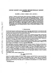
Figure 2. Histogram of 92 days’ outdoor temperature prediction errors for four typical hours from day-ahead 23:30 to the coming day.

As shown in Figure 2, the day-ahead predicted errors of outdoor temperature were recorded for 92 days from November 1, 2016, to January 31, 2017, in Beijing, based on data in [26]. It can be seen that the early time nodes show relatively less forecast deviation. The prediction errors of the zonal power, the summation of PV, and load are generated randomly with an asymmetric χ2 distribution,  P  0.15rand ( 52 )  0.75 for 5000 sample data for every h moment. We tested the performance of different N , P of the KDE function with power predicted errors as shown in

6 hN , P

Figure 3. This shows that a larger

may lead to a closer

KDE function with more burr. We finally chose and

hN ,T  0.1

hn = 0.01

hn = 0.1

Frequency

Frequency

0.5 -2 0 2 Prediction errors hn = 1

Frequency

1 0.5 -2 0 2 Prediction errors

4

xk ,t 1  0, if xk ,t  1 & Tw, k ,t  T w, k    xk ,t , other conditions

1 0.5 0 -4

4

1.5

Frequency

B. Comparison of KDEA-DRO with unscheduled conditions For unscheduled HP the ON/OFF 1, ifoperational xk ,t  0 & Tw,conditions, k , t  T w, k  state of the HP obeys a simple hysteresis rule: 

1.5

1

0 -4

and the average solving time for a KDEA-DRO problem was about 10 s.

for an appropriately smooth KDE function.

1.5

0 -4

hN , P  0.2

-2 0 2 Prediction errors hn = 10

(41)

4

The water temperature bounds

[T w, k , T w, k ]

were set

1.5

at [40,45] °C here. The results for KDEA-DRO and

1

unscheduled operation are shown in Figure 6 and Table 2. For the unscheduled scenario, Figure 6 shows that the transformer is overloaded from 17:30 to 19:30, when the electricity price is high. In contrast, the load profile of the transformer is flat and kept within its security limits with KDEA-DRO. Beyond that, HPs in the scheduled model turn off at high price moments to save money, and turn on at night for thermal energy storage, indicating good performance in load shifting. The large numerical differences of these models are shown in Table 3. The scheduled model cuts around 34% of the maximum daily transformer power and reduces the electricity cost for residents by about 18%.

0.5 0 -4

-2 0 2 Prediction errors

4

Figure 3. Histogram and KDE function of 5000 zonal power prediction errors

The predictions of PV power and the outdoor temperature curve are from real measurements on February 1, 2017, Tsinghua University, Beijing (Fig. 4). The TOU electricity price  is shown in Figure 5; the mean value is 1 $ / kWh . The penalty weight for transformer capacity  is 10 $ / kW for the test cases.

Unscheduled 80 Load Photovoltaic

30

Power (kW)

Power forecast (kW)

40

20

60 40 20

10

0 0

0

4

8

12 Time (h)

16

20

0

4

8

24

12

16

KDEA-DRO 60

20 24 Transformer Heat pumps

Power (kW)

Time of use electricity price ($)

Figure 4. Day-ahead PV and load prediction

2

40 20 0 -20

1.5

1

0

4

8

12 Time (h)

16

20

24

Figure 6. Operational power of transformer and heat pumps of the unscheduled model and KDEA-DRO model with y = 10 kW/$.

0.5

0

Table 2. Main results of unscheduled operational model and KDEA-DRO model 0

4

8

12 Time (h)

16

20

24

Figure 5. Curve of TOU electricity price

For the radius distance of the ambiguity set, we let t  t  2.3026, t for a 0.9 confidence level. Numerical experiments were conducted in MATLAB 2014b with a core-i7 laptop. The minimization of g ( ) was calculated by an inner-point method and the run time increased slightly when the historical data set increased. The mixed integer program was solved using CPLEX 12.5 with a 1% tolerance,

Peak cost ($)

Elec. cost ($)

Total ($)

Unscheduled

Pmax (kW) 73.204

732.0

962.7

1694.7

KDEA-DRO

48.612

486.1

787.6

1273.7

C. Comparison of deterministic, KDEA-DRO, GA-DRO, and RO models Operational strategies were generated using the deterministic, KDEA-DRO, GA-DRO, and RO models with the same setting and confirmed with 1000 Monte Carlo experiments. The intervals for RO were chosen with a 95% falling rate of

7

  

(42)

Table 3. Results of Monte Carlo experiments for the operational strategies generated with different models Method Best day Worst day Mean Best day Worst day Mean Best day Worst day Mean

Pmax /kW Elec cost /$ Comfo rt rate

Determin istic 44.38 47.9 47.18 734.4 818.8 801.7 100.0% 18.10% 85.6%

KDEA-D RO 45.82 49.34 48.62 702.8 787.2 770.1 100.0% 84.80% 93.7%

GA-DRO

RO

48.09 51.61 50.89 720.5 805 787.8 100.0% 86.90% 95.8%

48.76 51.27 50.56 725.7 810.1 793.0 100.0% 83.20% 94.1%

, which represent a robust part in the KDEA-DRO

model with different divergence settings. As shown in Figure 8, with the increase in divergence and the decrease in g g ( ) ( ) risk level, the P ,min and T ,t ,min increase with a gradually decreasing rate due to the robustness of the relative constraints. Due to the higher forecast accuracy, the gT ,6 h ,min ( ) is smaller than at the three other times (Fig. 8). gP,min(α) gT,6h,min(α)

1.8

gT,12h,min(α)

1.6

gT,18h,min(α)

1.4

gT,24h,min(α)

1.2

(α)

Num(t )

gT ,t ,min ( )

1 0.8

min

CRday  min  k  

  divergences t and t . As discussed in Section III, for an ambiguity set, the risk level  and the set’s divergence  , it  holds that   e . When the risk level increases to one, the divergence decreases to zero, and the DRO problem reduces to a stochastic optimization problem. g ( ) We first analyze the P ,min and four typical hours’

g

historical data and are symmetrical about zero (the concrete formulation of RO is shown in Appendix D). The forecast errors of outdoor temperature were generated by normally distributed random numbers, the means and variances of which were calculated from historical data, and the errors in power prediction were generated by the manipulated χ2 distribution mentioned above. The comfort rate (CR) is defined as the time between the comfort bounds divided by  Num(Tk  Tk ,t  Tk )  the total time.

0.6

Temperature (℃ )

Deterministic 40

0.2 0

20

indoor air 20

-0.2

Comfort bound 0

β=0.1

0

1

0 0

6

12

18

24

0 outdoor air

6

GA-DRO

Temperature (℃ )

0.4

KDEA-DRO water 40

40

40

20

20

0

0 0

6

12 Time (h)

12

18

24

RO

18

24

2

β=0.05

β=0.01

β=0.001

3 4 5 Divergence of the ambiguity set

6

7

8

Figure 8. gmin() of power and four typical hours prediction error data with different divergence η of the ambiguity set



0

6

12 Time (h)

18

24

Figure 7. Temperature simulations of deterministic, KDEA-DRO, GA-DRO, and RO model for 10 houses

From Table 3, we can see that the DRO methods have relatively high comfort satisfaction with less energy cost than the RO method. Because the uncertainties are not considered, the deterministic method has a poorer comfort rate and a P higher cost. Among the two DRO methods, max and the energy cost with KDEA-DRO are less than with GA-DRO, because the KDE function is more accurate than the Gaussian function in representing historical information, while the comfort satisfaction of KDEA-DRO is acceptable. Regarding the indoor comfort aspect, outage of indoor temperature of one house can be observed in the deterministic curves in Figure 7, while the robustness is better in the three robust methods. D. Discussion: Influence of the divergences

t

and

t

The ambiguity sets of the probability distribution of the uncertainties in our KDEA-DRO model are controlled by the



Next, we discuss the influence of divergences t and t on the results of KDEA-DRO via 1000 time Monte Carlo simulations; the other parameters are the same as those in subsection C. We select four risk levels. β = 0.1, 0.05, 0.01, and 0.001, for the power and temperature ambiguity sets for comparison; the outcomes are shown in Table 4. With the  increase in power divergence, t , the power peak increases, the electricity cost decreases, and the comfort rate rises. Thus, a large power divergence could provide an advantage in reducing the electricity cost and improving the users’ thermal satisfaction. Moreover, with an increase in outdoor  temperature divergence, t , the power peak increases slightly, the electricity cost increases, and the comfort rate rises. Based on these results, we can control the robustness and conservatism of the KDEA-DRO by varying the divergence settings. Table 4. Results of the KDEA-DRO under different   divergences of t and t for different risk levels β (a) Pmax (kW) t t

(risk level)

(risk level)

2.3026 (β = 0.1) 2.9957

2.3026 (β = 0.1)

2.9957 (β = 0.05)

4.6052 (β = 0.01)

6.9078 (β = 0.001)

48.62

49.51

52.11

52.21

48.37

49.42

51.27

52.37

 1    k   

(β = 0.05) 4.6052 (β = 0.01) 6.9078 (β = 0.001)

t

t

2.3026 (β = 0.1) 2.9957 (β = 0.05) 4.6052 (β = 0.01) 6.9078 (β = 0.001)

t

50.65

51.46

52.56

50.63

51.41

51.76

52.89

 k

  T   w, k  

k

   k   

8

 Tk ,t  0, set     T     out        . 

k

(b) Electricity cost ($) (risk level)

(risk level)

t

49.51

1

     T  k  k    1 

2.3026 (β = 0.1)

2.9957 (β = 0.05)

4.6052 (β = 0.01)

6.9078 (β = 0.001)

770.1

768.6

765.4

755.0

777.0

784.9

771.1

758.0

784.5

785.2

773.7

763.8

788.5

783.5

776.6

764.8

(45) This can be rewritten as

AkTk  BkTw, k  CkTout  d k

(46)

In the same way, we can state that

Ew, kTw, k  Fw, kTk  Gw, k xk  hw, k

It is easy to show that (c) Comfort rate (risk level)

(risk level)

2.3026 (β = 0.1) 2.9957 (β = 0.05) 4.6052 (β = 0.01) 6.9078 (β = 0.001)

and

Ew, k

(47)

are non-singular; thus,

we have

2.3026 (β = 0.1)

2.9957 (β = 0.05)

4.6052 (β = 0.01)

6.9078 (β = 0.001)

93.70%

95.47%

95.78%

96.02%

94.90%

95.52%

96.28%

96.31%

95.13%

95.68%

96.12%

96.42%

95.71%

95.71%

96.18%

96.50%

( Ak  Bk Ew1, k Fw, k )Tk  Bk Ew1,k Gw,k xk  CkTout  Bk Ew1,k hw,k  dk

( Ew, k  Fw, k Ak1Bk )Tw, k  Fw, k Ak1CkTout  Gw, k xk  hw, k  Fw, k Ak1d k

Due to the Schur complement, the matrices and

( Ew, k  Fw, k Ak1Bk )

Tk  J k xk  K kTout  lk

where

Tk

and

Tw, k

(50) (51) (52) (53)

Tw, k  M w, k xk  N w, kTout  pw, k

In this paper, we developed a KL distance-based DRO model of HP-DOSM with residential temperature constraints , which can both decrease the peak-valley gap and the cost to residents under a TOU electricity price. This distance-based DRO model can well capture the uncertainties of weather prediction, photovoltaic prediction, and load prediction errors, while it is tractable. Numerical tests showed that our distance-based DRO was robust with less conservatism than the conventional RO model. Moreover, the robustness of this model can be adjusted by tuning the risk level, which has an explicit meaning in the optimization problem. In future work, a distributed algorithm is needed to solve HP-DOSM for large-scale distribution networks integrated with massive heat pumps.

(49)

are non-singular, so we have:

Tw, k  ( Ew, k  Fw, k Ak1Bk )1 ( Fw, k Ak1CkTout  Gw, k xk  hw,k  Fw,k Ak1dk )

CONCLUSIONS AND FUTURE WORK

(48)

( Ak  Bk Ew1,k Fw, k )

Tk  ( Ak  Bk Ew1, k Fw, k )1 ( Bk Ew1, k Gw, k xk  CkTout  Bk Ew1, k hw, k  dk )

represented by V.

Ak

are decoupled.

B. Detailed reformulation of Gaussian Assumption and KDE Approximation in constraint (24) B.1 Gaussian Assumption (   ) The inner [formula  ]/  equals  x P  Pof  P(24) 1  / 2  ln  e e e d P ,t ]  t  P ,t 2 2

k ,t HP , k

Z sum ,t

P ,t

Z max

kZ

P ,t

Z Z   xk ,t PHP , k  Psum , t  Pmax   P , t  t  k Z

P ,t 2 P ,t

 P2 ,t 2

(54)

2 min{t  P ,t }   P ,t 2t 2 Due to   0 , we take (24) as Z x P   P ,t   P ,t 2t  0  k ,t HP,k  PsumZ ,t  Pmax k Z

(55)

APPENDIX A. Detailed structural transformation of the heat pump dayahead operational schedule model We first apply several simplifications. Transform the (3) and (4) equalities to a simplified form: Tk ,t 1   kTk ,t  kTw, k ,t   kTout ,t (43) Tw, k ,t 1   w, kTk ,t  w, kTw, k ,t  w, k xk ,t

B.2 KDE Approximation N The[  inner of x P formula P  P ]/  (24) equals 1  / 1  ln  e e  k ,t HP , k

kZ

Z sum ,t

Z max



P ,t

N P ,t

i 1

hN , P 2

Z Z   xk ,t PHP , k  Psum , t  Pmax  t  k Z

hN2 , P 2

  ln

(44)

With the definition of the vectors in the nomenclature, we have:

( P ,t  Pi ,t )2

e

P ,t

2 hN2 , P

1 N P ,t

d P ,t ]  t N P ,t

 Pi ,t

e  i 1

(56)

C. Convexity proof of g ( ) The convexity of g ( ) can be calculated by a second order differential function: h2 1 N  i

g ( )   

N

2

  ln

N

 e  ,  0 i 1

(57)

i 

9

N e   N     i 1e     i 1   2 hN2 g '( )    2  ln   i 2 N  N   e  2 i 1 i  i  N  i i 2 N e  ( )   i 1e      3 i  1 hN2     g ''( )  3  0 2 i i  N  N     e  i 1   i 1e      i

i

(58)

(59)

Thus, g ( ) is convex. D. Robust optimization model Z min (6) max  P  0  xk PHP , k  PsumZ  Pmax s.t.  [ , ] k Z P

P

P

max J k xk  K kTout  lk  Tk  K kT  0

T [T ,T ]

max  J k xk  KkTout  lk  Tk  KkT  0

T [T ,T ]

max Z0 (M w, k xk  N w, kTout  pw, k  N w, kT )  Tw, k ,t  0, set  0

T [T ,T ]

(60) (61) (62) (63)

(9), (11)(12)(14) xk ,t {0,1} t  1, , H , k  1,2, , N , Z , REFERENCES [1] C. R. Inc, "Heat pump characterization study," 2010. [2] EHPA, "European Heat Pump Association," Outlook European Heat Pump Statistics, 2011. [3] A. Arteconi, N. J. Hewitt, and F. Polonara, "Domestic demand-side management (DSM): Role of heat pumps and thermal energy storage (TES) systems," Applied Thermal Engineering, vol. 51, no. 1-2, pp. 155-165, 2013. [4] G. Z. C. D.-m. Y. J.-h. J. B. F. X.-m. Z. Liang, "Study on Rural Low-Voltage Distribution Network Planning with Coal-to-Electricity Project," Electrical & Electronics, 2015. [5] Xinhua. http://news.xinhuanet.com/local/2017-01/25/c_11203819 59.htm. [6] H. O. R. Howlader, H. Matayoshi, and T. Senjyu, "Distributed generation incorporated with the thermal generation for optimum operation of a smart grid considering forecast error," Energy Conversion and Management, vol. 96, pp. 303-314, 2015. [7] D. Vanhoudt, D. Geysen, B. Claessens, F. Leemans, L. Jespers, and J. Van Bael, "An actively controlled residential heat pump: Potential on peak shaving and maximization of self-consumption of renewable energy," Renewable Energy, vol. 63, pp. 531-543, 2014. [8] D. K. Wolfram Wiesemann, and Melvyn Sim, "Distributionally Robust Convex Optimization," 2013. [9] Y. Zhang, S. Shen, and J. Mathieu, "Distributionally Robust Chance-Constrained Optimal Power Flow with Uncertain Renewables and Uncertain Reserves Provided by Loads," IEEE Transactions on Power Systems, pp. 1-1, 2016. [10] S. Zymler, D. Kuhn, and B. Rustem, "Distributionally robust joint chance constraints with second-order moment

information," Mathematical Programming, vol. 137, no. 1-2, pp. 167-198, 2011. [11] P. Xiong, P. Jirutitijaroen, and C. Singh, "A Distributionally Robust Optimization Model for Unit Commitment Considering Uncertain Wind Power Generation," IEEE Transactions on Power Systems, vol. 32, no. 1, pp. 39-49, 2017. [12] E. D. a. Y. Ye, "Distributionally Robust Optimization under Moment Uncertainty with Application to Data-Driven Problems," Operation Research, 2008. [13] N. Loizou, "Distributionally Robust Game Theory," 2015. [14] D. K. Peyman Mohajerin Esfahani, "Data-driven distributionally robust optimization using the Wasserstein metric Performance guarantees and tractable reformulations," Optimization and Control, 2016. [15] R. Jiang and Y. Guan, "Data-driven chance constrained stochastic program," Mathematical Programming, journal article vol. 158, no. 1, pp. 291-327, 2016. [16] X. Chen and Y. Zhang, "Uncertain Linear Programs: Extended Affinely Adjustable Robust Counterparts," Operations Research, vol. 57, no. 6, pp. 1469-1482, 2009. [17] D. d. H. By Aharon Ben-Tal, Anja De Waegenaere, Bertrand Melenberg, Gijs Rennen, "Robust solutions of optimization problems affected by uncertain probabilities," 2011. [18] Z. Hu, Hong, L. Jeff, "Kullback-Leibler Divergence Constrained Distributionally Robust Optimization," Conference Proceedings, 2012. [19] K.-L. H. S. M. Manish Bansal, "Decomposition Algorithms for Two-Stage Distributionally Robust Mixed Binary Programs," 2017. [20] X. Li, K. Natarajan, C.-P. Teo, and Z. Zheng, "Distributionally robust mixed integer linear programs: Persistency models with applications," European Journal of Operational Research, vol. 233, no. 3, pp. 459-473, 2014. [21] W. Wu, Xin Chen, B. Zhang, C. Lin, "Data-driven DG Capacity Assessment Method for Active Distribution Networks," IEEE Transactions on Power Systems, 2016. to be published. [22] J. Tant, F. Geth, D. Six, P. Tant, and J. Driesen, "Multiobjective Battery Storage to Improve PV Integration in Residential Distribution Grids," IEEE Transactions on Sustainable Energy, vol. 4, no. 1, pp. 182-191, 2013. [23] J. Pintér, "Deterministic approximations of probability inequalities," 1989. [24] L. G. L. Devroye, "Nonparametric Density Estimation: The ℓ1 View," 1985. [25] Q. Z. Qisen Yan, Building thermal process. 1986. [26] http://data.cma.cn/site/index.html. China Meteorological Administration.