8th International Conference of Modeling and Simulation - MOSIM’10 - May 10-12, 2010 - Hammamet - Tunisia “Evaluation and optimization of innovative production systems of goods and services”
A LAGRANGIAN HEURISTIC METHOD AND AN ITERATIVE APPROACH FOR THE INVENTORY ROUTING PROBLEM Nadra B. TAARIT, Atidel B. HADJ-ALOUANE
Farah ZEGHAL MANSOUR
OASIS / ENIT B.P. 37, Le Belvédère, 1002 Tunis, Tunisia
[email protected] [email protected]
ROI / EPT BP 743, 2078 La Marsa, Tunisia
[email protected]
ABSTRACT: The inventory routing problem (IRP) deals with the integration of inventory decisions into the classical vehicle routing problem. In such a situation, the customer’s inventory is controlled by the supplier/distributor who decides on not only the vehicle routes but also on the quantities to be delivered to each customer. The objective is to minimize the total transportation and inventory holding costs while preventing customers’ stock-outs over a predetermined time horizon. In this paper, we consider IRP with heterogeneous vehicles and deterministic customer demand rates. The problem is formulated as a mixed integer program and its Lagrangian relaxation is solved to derive a lower bound. A Lagrangian based heuristic method is proposed to generate feasible solutions using Lagrangian solution information. An efficient iterative local search approach is also developed so as to obtain better solutions. Computational experiments show that the proposed iterative approach gives good solutions in reasonable computation times. KEYWORDS: inventory, routing, lagrangian relaxation, local search. 1
INTRODUCTION
The Inventory Routing Problem (IRP) combines two major logistics management decisions: inventory management and vehicle routing. These two stages of the supply chain are closely interrelated and their integration has been proved to lead to a better overall performance (Cousineau-Ouimet, 2002). Thus, instead of designing single day vehicle routes to deliver the customers' orders, the distributor and no longer the customer, decides when and in what quantities customers are delivered, based on their consumption rates. The objective is to minimize the total transportation and inventory holding costs over the planning horizon. The IRP has several industrial applications such as the petrochemical industry, the automotive industry, the grocery industry, the clothing industry, the blood collection service, etc. This is made possible thanks to technological advances in remote telemetry and communication that allow for monitoring customers inventory levels directly by the distributor. In response to today's extremely competitive market, designing efficient solution methods for the IRP has become an immediate necessity for many distribution industries. In fact, during the last twenty years, there is a growing interest in inventory routing and related problems in the literature. Various models have been proposed to deal with different variants of the IRP where assumptions are essentially related to the nature of demand and the time horizon. The IRP is stochastic when the demands of customers are uncertain. We refer to, among others, Adelman (2004), Federgruen and Zipkin (1984), Kleywegt et al. (2002), and Minkoff (1993). Such a problem is mostly
formulated as a Markov-decision process and is solved using dynamic programming or heuristic algorithms. In spite of the stochastic nature of the IRP input data, deterministic models have been extensively considered. The main reason is that, besides the complexity of the stochastic models solution approaches, it is often difficult to obtain the necessary information to derive probability distribution that represent the problem correctly. Since the IRP is a multi-period problem, the time horizon is a key parameter for its solution. Aghezzaf et al. (2006), Archetti et al. (2007), Campbell et al. (2002), Chien et al. (1989), and Yu et al. (2008) studied a multiperiod IRP where the decisions are carried out over a finite horizon. Anily and Federgruen (1993), Chan et al (1998), and Gallego and Simchi-levi (1990) considered infinite horizon problems where the decisions are limited to delivery frequencies. We should note that most of studies dealing with the infinite horizon problem use a distribution policy that is similar to the fixed partition policy (first introduced by Anily and Federgruen (1993)), direct deliveries, order-up-to level policy and zero-inventory ordering (Bertazzi et al. (2002), Chan et al (1998)). To solve the IRP, most research works have focused on heuristic solution approaches due to its NP-hard complexity. Frequently, the integrated problem is decomposed into subproblems which are solved by approximate or exact methods (i.e. Branch and Cut, column generation). In some cases, heuristic methods are applied to the subproblems in order to identify upper and lower bound. Some of the studies provided integrated and iterative approaches and evaluated the effectiveness of
8th International Conference of Modeling and Simulation - MOSIM’10 - May 10-12, 2010 - Hammamet - Tunisia “Evaluation and optimization of innovative production systems of goods and services”
integrating routing and inventory decisions in their models. Others proposed heuristic methods to be compared with approaches used in industry (Campbell et al. (2002), Dror and Ball (1987)).
The transportation cost is composed of two terms that express the usage cost of a vehicle vV to travel from customer location i K to customer location j K in
In this paper, we consider the repetitive distribution of a single product from a single depot to a set of customers, using a fleet of heterogeneous vehicles over a given finite horizon. Each customer consumes the product at a deterministic rate and has limited storage capacities, while the depot has an unlimited supply and a large storage capacity for the product. Thus, the problem consists in determining, for each day of the horizon, the customers’ delivery quantities as well as vehicle routes, so as to minimize the total transportation and inventory holding costs. Additional realistic constraints are considered to prevent customers’ stock-out and prohibit the same vehicle from visiting each customer more than once a day. This IRP variant represents a real problem encountered by a Tunisian petrochemical company that pumps the product via a pipeline and ensures its distribution to its service stations.
The first cost includes the fixed usage costs as well as variable shipping costs that depend on traveled distance whereas the second cost includes the variable shipping costs that depend on transported quantity and traveled distance.
The objective of this paper is to develop fast and efficient heuristic approaches for solving the considered real world IRP variant. The innovative feature of these approaches is that they combine well-known network flow techniques and Vehicle Routing Problem basic heuristics. Moreover, we develop Lagrangian based lower bounds using a multi-commodity model. Computational experiments demonstrate the effectiveness of the proposed heuristics. The remainder of this paper is organized as follows. In Section 2, we present a valid multi-commodity network flow formulation. In Section 3, we propose a Lagrangian based approach for solving the considered IRP. In Section 4, we describe a two-phase heuristic method for the IRP. Computational results are presented and discussed in Section 5. Finally, we provide some concluding remarks. 2 A MULTICOMMODITY NETWORK FLOW FORMULATION Let T, indexed by t, be the set of consecutive days of the considered planning horizon. Let K, indexed by i and j, be the set of customers where 0 represents the depot. Each customer i K is characterized by its initial inventory level I i0 , its storage capacity Ci, its unit holding cost h tj per unit of product in period t and its demand
rate u it in period t T . Let V, indexed by v, be the set of heterogeneous vehicles with limited capacity CAPv, vV. These vehicles are located at the depot, and consequently routes must depart from and then return to the depot.
day t T : a fixed cost CF ijvt and a variable cost CV ijvt .
This transportation cost structure, first adopted by Fumero and Vercellis (1999) and then by others such as Yu et al. (2008), reflects the transportation pricing in practice.
We define the following decision variables:
Sit : the product quantity to be delivered to customer i K in day t T . Yijvt : a binary variable that equals 1 if vehicle v V serves customer j K immediately after customer i K in day t T and 0 otherwise. X ijvt : the product quantity carried by vehicle v V from customer i K to customer j K in day t T . Using these notations, we formulate the IRP as the following mixed integer linear program (P). (P)
Min
CFijvt Yijvt CVijvt X ijvt
t T j K i K vV
htj ( S sj tT jK
1 s t
u sj I 0j )
1 s t
(1)
Subject to
t X ijv CAP .Yijvt , j,i K,i j , vV,t T ,
S
1 s t
S
1 s t
Cj u sj I 0j , t T , j K , 1 s t s s 0 u j j I j , t T , j K , 1 s t
s j
(2) (3) (4)
Xijvt X tjiv S tj , t T,j K, j 0, (5)
iK vV i j
iK vV i j
X it0v X 0t iv Sit , t T ,
iK vV i0
Y ijvt
i K i j
i K Sit
t X ijv
iK vV i0
Y jivt
i K i j
i K i 0
0 , t T, j K, v V , (7)
Y ijvt 1 , v V , j K , t T ,
0,
(6)
i K , t T ,
0 , j,i K,i j , vV,t T ,
(8) (9) (10)
8th International Conference of Modeling and Simulation - MOSIM’10 - May 10-12, 2010 - Hammamet - Tunisia “Evaluation and optimization of innovative production systems of goods and services”
Yijvt 0,1 , j,i K,i j , vV,t T .
(11)
The objective function (1) minimizes the transportation and holding cost where
s1 S sj s1u sj I 0j t
t
is the
inventory level of customer j in period t. Constraints (2) state the vehicle capacity restrictions. Constraints (3) express the inventory capacity constraints for each customer. Constraints (4) prevent stock-outs over the planning horizon. Constraints (5) and (6) are the product flow conservation constraints at customers and depot respectively. Constraints (7) express the vehicle flow conservation constraints and at the same time, they compel each vehicle to return to the depot after visiting all its customers. We observe that constraints (5)-(7) together with constraints (2) eliminate sub-tours. On one hand, these constraints prevent visiting a customer without delivering him some amount of product and on the other hand, they allow for loading products only at the depot. Thus, all tours must include the depot and sub-tours are eliminated. Constraints (8) limit the visits of each vehicle to each customer to at most once a day. Constraints (9)-(11) are the integrality and sign constraints to be imposed on the variables. The mixed integer program (P) has a large number of variables and constraints that make it difficult to be solved optimally in a reasonable computation time. Therefore, we develop a Lagrangian based approach that generates both lower and upper bounds. 3 A LAGRANGIAN BASED APPROACH
Figure 1: Lagrangian based approach 3.1 Relaxation and decomposition Constraints (5) and (6) of the mixed integer program (P) are considered as the complicating ones since they combine inventory allocation variables S and flow variables X . Therefore, we propose to relax these constraints and to incorporate them in the objective function using unsigned Lagrangian multipliers
A set of complicating constraints is first relaxed in order to enable the decomposition of the problem into an inventory allocation subproblem and a vehicle routing subproblem. These subproblems are solved to optimality and then a sub-gradient algorithm is applied to update the Lagrangian multipliers and therefore derive a lower bound on the optimal solution of the original program (P). A heuristic method is also included so as to generate feasible solutions for program (P) (see figure 1).
The
resulting relaxed problem (RP) is stated as follows.
CFijvt Yijvt CVijvt tj ti Xijvt
(RP): To solve the proposed mixed integer program (P), we propose a Lagrangian based approach that iteratively produces a lower and an upper bound for the optimal solution of (P).
tj , t T,j K .
Min
tT jKiK vV
tT jK
tj S tj
tT
tT jKiK vV
t0
S tj
jK
htj ( S sj tT jK
1 s t
u sj I 0j )
(12)
1 s t
Subject to (2)-(4), (7)-(11). The relaxed problem (RP) can be decomposed into two independent subproblems: an inventory allocation subproblem (INV) and a vehicle routing subproblem (ROU). Furthermore, subproblem (INV) can be decomposed into independent subproblems, each corresponding to a customer. Let (INV)j be the subproblem associated with customer j, which can be stated as follows. Min
(tj t0 )S tj htj ( S sj u sj I 0j )
tT
(13) Subject to
tT
1 s t
1 s t
8th International Conference of Modeling and Simulation - MOSIM’10 - May 10-12, 2010 - Hammamet - Tunisia “Evaluation and optimization of innovative production systems of goods and services”
S sj C j u sj I 0j , t T,
1 s t
S
s j
1 s t
1 s t u sj I 0j 1 s t
, t T ,
t T.
S tj 0,
(14)
by Branch-and-Bound, using standard optimization software (i.e. CPLEX).
(15)
3.2 Lower bound computation
(16)
Solving the set of relaxed subproblems (INV)j, j K ,
Observe that the obtained subproblems (INV)j, j K , are inventory allocation problems that can be efficiently solved to optimality by the simplex method for linear programming. In order to decompose subproblem (ROU) by location j K and by day t T , Constraints (7) must also be relaxed. Let jv , t T, j K, v V be the unsigned t
corresponding Lagrangian multipliers. Moreover, valid constraints (17) and (18) are appended to the model so as to enhance the relaxed and decomposed subproblems. t X ijv Yijvt , j,i K,i j, j 0, vV,t T
i K v V i j
X
1 ijv
u 1j
I
0 j
, j K , j 0
(17) (18)
Subproblems (ROU) , j K , t T , can be stated as
follows:
Min
tT i K jK vV
CFijvt
tjv
CVijvt tj tT iK jK vV
X
ivt t i
Yijvt t ijv
(19)
Subject to
t X ijv CAP .Yijvt , i K,i j , vV,
i K
Y ijvt 1 ,
t X ijv Yijvt ,
i K v V i j
t X ijv
X
0,
1 ijv
u 1j
v V ,
i K,i j, , vV, I ,
(DP) Max L( j , 0 , jv ) t
t
t
where L( j , 0 , jv ) = t
t
t
CFijvt tjv ivt Yijvt
Min
tT iK jK vV
t CVijvt tj ti X ijv
tT iK jK vV
tj S tj t0 S tj
tTjK jK
tT
htj ( S sj 1 s t tT jK
j K
u sj I 0j )
(26)
1 s t
To solve problem (DP), the most popular method is the sub-gradient algorithm (Sherali and Ulular (1990)). It attempts to improve the value of L( j , 0 , jv ) by t
t
t
finding, iteratively, good directions for updating the Lagrangian multipliers. 3.3 Lagrangian Heuristic Method The Lagrangian relaxation approach produces lower bounds for the original problem (P). In this procedure, several constraints are relaxed, and using appropriate Lagrangian multipliers values, these constraints are recovered iteratively. Therefore, solutions generated at each iteration, are not feasible for problem (P).
(20) (21) (22)
0 j
(23)
i K,i j , vV,
(24)
Yijvt 0,1 , i K,i j , vV.
the optimal solution of the original problem (P), for any given Lagrangian multipliers. The best lower bound can be obtained by the optimal Lagrangian multipliers, solution of the following Lagrangian dual problem (DP).
is the solution value of (RP).
Constraints (17) prevent visiting a customer with no delivery. Constraints (18) prohibit stock-outs during the first day of the planning horizon. t j
(ROU) tj , j K , t T , gives a lower bound to
and
(25)
Subproblems (ROU) tj , j K , t T , are mixed integer programs with fewer variables and constraints than the original routing problem. These subproblems are solved
To build feasible solutions, we develop a heuristic method that exploits the Lagrangian information and, at each iteration, derives a feasible solution for problem (P), using the solution of the subproblems (INV)j,
j K , and (ROU) tj , j K , t T .
The optimal solutions of subproblems (INV)j, j K , provide the product quantities to be delivered to each customer at each day of the planning horizon. These quantities are considered as customer orders and a vehicle routing problem is solved for each day separately using an extension of the savings algorithm to a heterogeneous fleet of vehicles (Clarke and Wright (1964), Rego and Roucairol (1994)). It consists in assigning each customer to a separate route, and then combining routes
8th International Conference of Modeling and Simulation - MOSIM’10 - May 10-12, 2010 - Hammamet - Tunisia “Evaluation and optimization of innovative production systems of goods and services”
according to their decreasing savings until no more combinations are feasible. A combination is infeasible if it violates the capacity constraints. Hence, at each iteration of the Lagrangian relaxation approach, we derive, from the modified delivery schedule obtained by the updated lagrangian multipliers, a feasible solution that is an upper bound for the problem (P). To improve this solution we apply the improvement procedure of the iterative local search method described in paragraph 4.2. 4 AN ITERATIVE LOCAL SEARCH HEURISTIC APPROACH In this section, we describe an iterative local search approach that solves the IRP by applying two consecutive procedures: a building procedure followed by an improvement procedure. These two procedures are embedded into an iterative local search scheme. 4.1 Building Procedure The IRP is decomposed into an inventory allocation subproblem and a vehicle routing subproblem that are solved sequentially. For each customer, the inventory allocation subproblem is formulated as a minimum cost flow problem. Let Gj = (D, A) be a network associated to customer j K , where D is the set of nodes and A is the set of arcs. Each day of the planning horizon is represented by a node in D. Two dummy nodes O and P are also defined. The set A is composed of three types of arcs: (1) delivery arcs that link the origin node O to each day t T . Each of these arcs has a capacity of u tj + Cj and a cost of
tj t0 , (2) inventory arcs that link each day t T
to
the next day t 1T . Each of these arcs has a capacity of Cj and a holding cost of h tj per unit of product, and
(3) demand arcs that link each day t T to the sink node P. The capacity on each of these arcs is u tj - I tj and their cost is null. The inventory allocation problem is then solved, for each customer j K , as a minimum cost flow problem on the corresponding network Gj. Using the obtained product quantities as customer orders, we solve a vehicle routing problem for each day of the planning horizon using an extension of the savings algorithm to a heterogeneous fleet of vehicles (Clarke and Wright (1964), Rego and Roucairol (1994)). 4.2 Improvement Procedure To improve the obtained initial solution, we propose time and space adjustments that are applied only if the cost is reduced while satisfying all the constraints:
Inter-days fusion: for each customer that is planned to be served in two consecutive days, the total quantity to be delivered is scheduled in the former day so as to avoid visiting him twice. Inter-days insertion: deliveries scheduled for a given day are inserted in previous days’ routes. Intra-routes exchange: an r-arcs exchange procedure is applied to each route (Lin and Kernighan, 1973). 4.3 Iterative local search When solving the inventory allocation subproblem and the vehicle routing subproblem separately, the solution tends to reduce inventory costs by delivering products in a just-in-time strategy, which increases the transportation costs. To find a trade off between these two conflicting
costs, we propose to compute the total cost ( tci ) of vist
iting each customer i K in a day t T , according to the initial solution and then introduce this cost in the inventory allocation subproblem. The process is then reinitiated and the building procedure followed by the improvement procedure, are applied again. The total cost ( tci ) of visiting each customer i K in a t
day t T , is considered as the additional transportation cost that is required to insert customer i in a route in day t. 5
COMPUTAIONAL RESULTS
To evaluate the performance of the proposed heuristics, computational experiments were carried out on randomly generated instances according to the Yu et al. (2008) generation scheme. The locations of the depot and the customers are generated uniformly from the square [0,10]2 and Euclidean distances are used to measure vehicle routing costs. The demand rate and the inventory capacity of each customer are randomly and uniformly generated respectively from the intervals [50,400] and [400,800]. The vehicle capacities are randomly generated from the interval [800, 1200] and the number of vehicles is selected as serving the total demand of all customers to make the problem feasible. The planning horizon is composed of 3 consecutive days (T=3). We consider a variant that represents a real problem encountered by a Tunisian petrochemical company that pumps the product via a pipeline and ensures its distribution to its service stations. In this case, the customers are part of the same company, and consequently the inventory costs are null. We consider different sets of problem instances with different customer and vehicle sizes. Each problem set is identified by the number of customers N and vehicles M respectively. The three tested problem sets are: (N=10, M=4), (N=20, M=6) and (N=50, M=12). Moreover, for
8th International Conference of Modeling and Simulation - MOSIM’10 - May 10-12, 2010 - Hammamet - Tunisia “Evaluation and optimization of innovative production systems of goods and services”
All the proposed approaches were coded in the C++ programming language using the callable library of CPLEX 11.0 and were run on a Pentium IV PC with 1.73 GHz processor and 512 Mo of RAM. Tables 1-3 give the results obtained by the Lagrangian based method and the iterative local search approach for each of the three considered problem sets respectively. Each table provides the following measures: LHGAP(%): the gap, in percentage, between the upper bound obtained by the Lagrangian based method and the Lagrangian lower bound. IHGAP(%): the gap, in percentage, between the upper bound obtained by the iterative local search approach and the Lagrangian lower bound. IH CPU(seconds): the CPU time required by the iterative local search heuristic approach. This time does not include the Lagrangian lower bound computation. The percentage gap is defined as (UB- LB)*100/ LB, where UB is the heuristic upper bound and LB is the best Lagrangian lower bound. IH CPU Instances LHGAP(%) IHGAP(%) (seconds) 1 0.06 0.06 0.094 2 0.15 0.31 0.063 3 0.04 0.04 0.156 4 0.04 0.04 0.125 5 0.09 0.13 0.125 6 0.04 0.04 0.062 7 0.1 0.1 0.078 8 0.04 0.04 0.125 9 0.03 0.03 0.078 10 0.04 0.04 0.093 Average 0.06 0.08 0.099 Table1: Results of (N=10, M=4) set problem instances IH CPU Instances LHGAP(%) IHGAP(%) (seconds) 1 0.11 0.11 0.250 2 0.12 0.29 0.219 3 0.08 0.08 0.250 4 0.25 0.26 0.219 5 0.08 0.08 0.234 6 0.04 0.11 0.281 7 0.11 0.11 0.234 8 0.1 0.20 0.235 9 0.18 0.18 0.266 10 0.18 0.25 0.328 Average 0.13 0.16 0.251
Table2: Results of (N=20, M=6) set problem instances
IH CPU Instances LHGAP(%) IHGAP(%) (seconds) 1 0.11 0.11 1.797 2 0.29 0.29 1.922 3 0.26 0.26 1.891 4 0.27 0.42 0.829 5 0.15 0.25 0.938 6 0.57 0.57 0.828 7 0.39 0.39 1.250 8 0.77 0.83 2.375 9 0.41 0.41 1.766 10 0.3 0.81 0.922 Average 0.35 0.43 1.451 Table 3: Results of (N=50, M=12) set problem instances The results demonstrate the effectiveness of the iterative local search heuristic approach. It gives near optimal solutions that are, in average, within 0.08%, 0.16% and 0.43 % of the lower bound for the (N=10, M=4), the (N=20, M=6) and the (N=50, M=12) problem sets respectively as it is shown on figure 1. In the worst case, the gap between the obtained feasible solution and the lower bound is 0.83%. Moreover, the iterative local search method provides solutions in less than 2.5 seconds. We observe that the Lagrangian based approach requires much more computation time to derive good quality lower bounds (2 hours for (N=20, M=6) instances) due to the large number of linear programs that need to be solved. This drawback is accentuated for large scale problems. The best feasible solution found by the Lagrangian based heuristic approach is also reached by the iterative local search approach for 19 instances while requiring more than 2 hours computation time against less than 2.5 seconds for the iterative local search approach.
GAP (%)
each problem set, ten instances are generated.
0,5 0,45 0,4 0,35 0,3 0,25 0,2 0,15
LHGAP(%) IHGAP(%)
0,1 0,05 0 (N=10,V=4) (N=20,V=6) (N=50,V=12) Instance type
Figure 1: Average LHGAP and IHGAP
8th International Conference of Modeling and Simulation - MOSIM’10 - May 10-12, 2010 - Hammamet - Tunisia “Evaluation and optimization of innovative production systems of goods and services”
5
CONCLUSION
In this paper, we considered a multi-period deterministic inventory routing problem that determines the delivery schedule and the routing plan of a heterogeneous fleet of vehicles. The objective is to minimize the product transportation costs over the planning horizon, without causing stock-outs. A Lagrangian based method is proposed to derive both lower and upper bounds for the considered IRP. An efficient iterative local search heuristic approach is also developed to provide good quality feasible solutions (less than 0.9% of the lower bound) in reasonable computation times (less than 2.5 seconds for the tested instances). This research is currently being extended to different variants of the inventory routing problem such as multi-product inventory routing problems and problems with stochastic demands. REFERENCES Adelman, D., 2004. A price-directed approach to stochastic inventory/routing, Operations Research, vol. 52, p. 499-514. Aghezzaf, E. H., B. Raa, , H. Van Landeghem, 2006. Modeling inventory routing problems in supply chains of high consumption products. European Journal of Operational Research ,vol. 169 (3), p. 1048-1063. Anily, S. and A. Federgruen, 1993. Two-Echelon Distribution Systems with Vehicle Routing Costs and Central Inventories, Operations Research, vol. 41, p. 3747. Archetti, C., L. Bertazzi, G. Laporte, M. G. Speranza, 2007. A Branch-and-Cut Algorithm for a VendorManaged Inventory-Routing Problem, Transportation science, vol. 41, p. 382-391.
Chien, T. W., A. Balakrishnan, and R. T. Wong, 1989. An integrated inventory allocation and vehicle routing problem. Transportation Science, vol. 23, p. 67-76. Clarke, G.. and J. Wright, 1964. Scheduling of vehicles from a central depot to a number of delivery points, Operations Research, vol. 12, p. 568-81. Cousineau-Ouimet, K., 2002. A Tabu Search Heuristic for the Inventory Routing Problem, Proceedings of 37th
Annual ORSNZ Conference.
Dror, M. and M. Ball, 1987. Inventory/Routing: Reduction from an Annual to a Short-Period Problem, Naval Research Logistics, vol. 34, p. 891-905. Federgruen, A. and P. Zipkin, 1984. A combined vehicle routing and inventory allocation problem, Operations Research, vol. 32, p. 1019-1037. Fumero, F. and C. Vercellis, 1999. Synchronized development of production, inventory, and distribution schedules. Transportation Science, 33 (3), p. 330–340.
Gallego, G. and D. Simchi-Levi, 1990. On the Effectiveness of Direct Shipping Strategy for the OneWarehouse Multi-Retailer R-Systems, Management Science, vol. 36 (2), p. 240-243. Kleywegt, A., V. Nori and M. Savelsbergh, 2002. Dynamic programming approximations for a stochastic inventory routing problem. Technical Report TLI-0206, Department of Industrial and Systems Engineering, Georgia Institute of Technology, Atlanta, GA. Lin, S. and W. Kernighan, 1973. An Effective Heuristic Algorithm for the Travelling-Salesman Problem, Operations Research, vol. 21, p. 498-516. Minkoff, A. S., 1993. A Markov Decision Model and Decomposition Heuristic for dynamic Vehicle Dispatching, Operations Research, vol. 41, p. 77-90.
Bertazzi, L., G. Paletta, and M. G. Speranza, 2002. Deterministic order-up-to level policies in an inventory routing problem, Transportation Science, vol. 36, p. 119-132.
Rego, C. and C. Roucairol, 1994. Le problème de tournées de véhicules: études et résolution approchée. Rapport de recherche, No. 2197, Institut National de Recherche en Informatique et en Automatique, France.
Campbell, A, L. W. Clarke, and M. Savelsbergh, 2002. Inventory Routing in Practice. The Vehicle Routing Problem, edited by Paolo Toth and Daniele Vigo. Philadelphia : Society for Industrial and Applied Mathematics, p. 309-330.
Sherali, H. D. and O. Ulular, 1990. Conjugate Gradient Methods Using Quasi-Newton Updates with Inexact Line Searches, Journal of Mathematical Analysis and Applications, vol. 150, p. 359-377.
Chan, L. M. A., A. Federgruen, and D. Simchi-Levi, 1998. Probabilistic Analysis and Practical Algorithms for Inventory-Routing Models, Operations Research, vol. 46(1), 96-106.
Yu, Y., H. X. Chen and F. Chu, 2008. A new model and hybrid approach for large scale inventory routing problem, European Journal of Operational Research, vol. 189, p. 1022-1040.